Adaptive geometric median prototype selection method for k-nearest neighbors classification

Abstract

The k-nearest neighbors (kNN) algorithm is one of the most popular and simplest lazy learners. However, as the training dataset becomes larger, the algorithm suffers from the following drawbacks: large storage requirements, slow classification speed, and high sensitivity to noise. To overcome these drawbacks, we reduce the size of the training data by only selecting the necessary prototypes before the classification. This study proposes an extended prototype selection technique based on the geometric median (GM). We compare the proposed method with seven state-of-the-art prototype selection methods and 1NN as the baseline model. We use 25 datasets from the KEEL and UCI dataset repository website. The proposed method runs at least 3.5 times faster than the baseline model at the cost of slightly reduced accuracy. In addition, the classification accuracy and kappa value of the proposed method are comparable to those of all the state-of-the-art prototype selection methods considered.

Keywords

Data pre-processing nearest-neighbors classification prototype selection instance selection

1. Introduction

The k-nearest neighbors classifier (kNN) is a popular instance-based learning classifier. It is easy to understand and implement because classifying unseen data is done by distance calculation and counting. Because kNN is simple and guarantees a low error rate [24], it is widely implemented in data mining and machine learning research. However, kNN has the following disadvantages when used with a huge dataset: 1) it requires large memory space for storing all training instances, 2) it is slow to classify due to its inefficient learning design and 3) it is highly sensitive to noise when the training data contains noises and outliers [17].

The above weaknesses have been studied and handled using many approaches. Data reduction techniques can help a kNN classifier to overcome these drawbacks by reducing the size of the training set. Most algorithms need to search an entire dataset for a set of nearest neighbors for each sample. Even though the nearest neighbors searching process helps such algorithms to create a list of all possible candidates to be selected, it takes a very long time to finish on a large dataset. Therefore, it is still not practical to use these algorithms to classify kNN with a large dataset.

To speed up the selection process, the geometric median prototype selection (GMPS) method is a data reduction method for a kNN classifier that uses the geometric median (GM) as a class prototype [2]. GM minimizes the sum of the distances to other instances. The GMPS method provides better performance than seven other state-of-the-art methods. The GMPS method runs approximately five times faster than the 1NN classifier model with near equal accuracy. Moreover, one important parameter for the algorithm, GMPS partition size, has to be assigned manually. The suitable partition size depends on the features of each dataset, so a human assessor randomly inputs a partition size to test the performance of the GMPS method. This is an expensive task, especially if this process is repeated until an appropriate partition size is found. Thus, this is impractical when this method is applied to unseen datasets. This paper aims to propose another version of the GMPS method that selects a suitable partition size automatically. The proposed method adds Appropriate partition size assignment (APSA) process that calculates the suitable partition size for each dataset. The APSA process helps the proposed method adapted for any unseen datasets.

The paper is organized as follows. The previous prototype selection (PS) methods are reviewed in Section 2. The new APSA method is proposed in Section 3. The details of the experimental setup are explained in Section 4. Finally, the empirical results and future work relating to this research are discussed in Section 5.

2. Related work

Data reduction techniques decrease the complexity of huge datasets in the execution of data mining algorithms. The reduced datasets still contain the quality of actual knowledge of the original datasets. For a kNN classifier, data reduction techniques can reduce memory consumption and speed-up the classification process. Data reduction techniques can be classified into two major groups: prototype generation and prototype selection, where the prototypes are samples selected from the original dataset by data reduction techniques. A prototype generation (PG) method generates new artificial prototypes by summarizing a number of similar instances and replacing the original training set because PG methods intensively create artificial instances which have different values from the original data [28]. The set of artificial instances can only be used as a training set for classification, not for other purposes. A prototype selection (PS) method selects a subset of the original training instances into prototypes. The PS method has efficient real data handling and low memory usage. The PS method is efficiently applied on many real-world applications. In general, PS methods consume less memory and runs faster than PG methods. PG methods compute several mathematical or statistical functions to summarize the intrinsic knowledge for artificial data generation while PS techniques keep representative data from the original training set by detecting border points or removing noisy instances [18, 21]. There are three types of prototype selection: condensation, edition, and hybrid.

Condensation selection focuses on keeping samples near the decision boundaries. The decision boundary is the region that separates the underlying instances into two sets: one for the concerned class and another for the rest. A sample that is near the decision boundary is called a border point. Condensation selection retains border points by removing internal instances that have little effect on the accuracy of the classifier model. The Condensed Nearest Neighbor (CNN) algorithm is the first well-known condensation method [25]. It focuses on the selection of a consistent subset of the original dataset. The sample that is correctly classified according to its nearest neighbors is removed and the remaining samples become members of the consistent subset. CNN tries to retain class border samples and remove internal samples because the misclassified data normally are located close to the decision boundary. The RNN algorithm [12] extends the concept of CNN by finding a minimally consistent subset. Both of these methods use the same removal criteria but RNN builds the edited set from the opposite direction by starting from a full training set and removing samples that are classified correctly. Furthermore, Fast Nearest Neighbor Condensation (FCNN), a fast condensation method, selects the centroid of each class in the training set and continues to insert a representative of the misclassified samples of each Varonoi cell [10]. The RNN method is the more costly but it provides a slightly smaller subset than CNN method. The FCNN method is at least twice as fast as the CNN and RNN methods with comparable classification accuracies and reduction rates. The condensation methods produce small subsets but they are sensitive to noise.

The edition scheme focuses on removing misclassified samples which is the opposite of the condensation method. Edited Nearest Neighbor (ENN) [4] was the first edition algorithm that followed the Wilson Editing rule, according to which, all instances that are incorrectly classified in the same class as their nearest neighbors are assumed to be noisy samples. ENN initially creates a subset of the same size as the original training set. ENN iteratively removes samples from the subset that are misclassified in the original training set. In other words, it attempts to remove samples that are noisy or disagree with their neighbors. Overall, ENN removes noise very with high level of accuracy but the number of reduced instances is low. However, there are several edition methods based on modifications of the ENN concept such as Repeated ENN (RENN) and All-kNN [14]. The reduction rate of the extended methods is better than that of ENN but their accuracy is similar or worse.

Hybrid methods are popular because they remove noise better than condensation methods and reduce the dataset more than edition methods. Also, the classifier models are more accurate than hybrid methods having condensation and edition methods on their own. Hybrid methods try to remove the internal and border points using the criteria of the other types. Instance Based Learning (IB3) [7], the first method in this category, starts by incrementally creating a classification record with a summary of a sampleæŠ¯ classification performance such as the number of correct and incorrect classification attempts. Keeping this classification record facilitates good classification performance with each sample. IB3 removes noise which has a poor classification record and a detrimental effect on significance testing later on. Decremental Reduction Optimization Procedure (DROP3) [5] uses a noise-filtering process based on a rule similar to ENN. Samples in the training set are first classified by the majority vote of their neighbors, after which the misclassified samples are removed. This helps to remove noisy samples and smooth the decision boundary. The points far from the decision boundary are also removed using distance sorting to the nearest enemy. In addition, Iterative Case Filtering (ICF) [13] improves the idea of DROP3 by building two local sets: coverage and reachability. The coverage set is the set of all samples closer to the sample $x$ than its closest enemy, defined as the nearest neighbor of a different class. The reachability set is the set of all samples that have sample $x$ as one of the nearest neighbors. ICF continually removes samples where the size of the reachability set is greater than the size of the coverage set. This removal helps to eliminate samples that generalize information from other samples.

Moreover, some hybrid methods utilize graph techniques to present the training set as a network of nearest neighbors. The Hit Miss Networks (HMN) method [8] proposes a graph-based representation of a training set that includes a short description of the nearest neighbors connection between pairs of samples. The graph has a directed edge from each sample to the nearest neighbors of each different class, with one edge per class. The structure attributes of the HMN graph correspond to attributes of samples related to the decision boundary of the 1NN rule such as the border point or central point. There are two main functions to evaluate how far a sample is located from the decision boundary: hit-degree and miss-degree. The hit-degree of a node is computed as the number of edges directed to the same class node. The miss-degree is computed in the opposite way to a hit-degree. HMN-EI, the most effective version of HMN, deletes samples or nodes which have no incoming edges in the first place. Then, it iteratively compares and removes samples if the miss-degree value is greater or equal than the hit-degree value. Moreover, Class Conditional Instance Selection (CCIS) [9] extends the concept of HMN network graph. Consequently, CCIS provides two graphs: the between-class and the within-class nearest neighbor graphs. These graphs are used to define a new margin scoring method for sample selection. There are two phases to this method. First, the Class Conditional selection (CC) process removes the outliers, isolated points, and points close to the 1NN decision boundary. Second, the Thin-out selection phase focuses on selecting a small number of instances without any additional 1NN error.

The data reduction techniques have high computational complexity because they generate artificial prototypes or collect sets of instances from a large dataset such as border instances and internal instances [32]. Most PS algorithms in the three selection schemes select each sample by its nearest neighbor’s classification scores or the margin values of its neighbor’s connection graph. The nearest neighbors searching process takes a long time to finish on a large dataset. The proposed method aims to improve the speed of the prototype selection process by selecting only a set of median points in each partition of the dataset.

3. Adaptive geometric median prototype selection (AGMPS)

This section describes the principle and hypothesis of the Adaptive Geometric Median Prototype Selection (AGMPS) algorithm for kNN classification. Figure 1 shows the process flow of the AGMPS algorithm. AGMPS combines Appropriate Partition Size Assignment (APSA) as a suitable measuring method for the partition size, and geometric median prototype selection (GMPS) as the GM searching method. The first process calculates a suitable partition size for each dataset and passes it on to the next process. The second process uses the number of partitions for splitting the dataset and selecting GM points as class representatives.

The APSA process fits a quartic polynomial function with a list of two dimensional Cartesian coordinates, where the $x$ coordinate is the partition size and the $y$ coordinate is the average distance between the other samples and each GM in $x$ partitions. A root of derivative polynomial function is chosen as the number of appropriate partitions. The APSA process helps the proposed method to adapt to any unseen datasets.

Figure 1.

The process flow of AGMPS algorithm.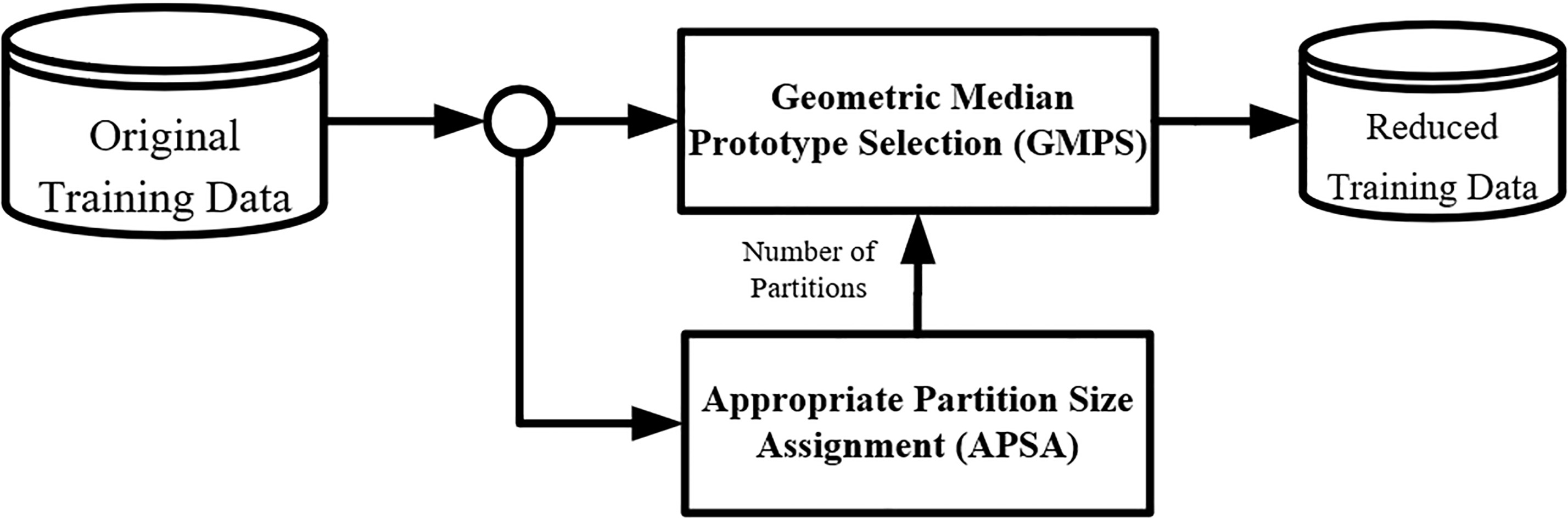

3.1 Geometric median

The GM of sample points in a Euclidean space is the sample point that minimizes the sum of distances to all other sample points. The GM is a robust measure of central tendency because it is not excessively affected by outliers. Formally, for a given set of $n$ points $S$ $=$ $\{x_{1},x_{2},\ldots,x_{n}\}$ with each $x_{i}\in R^{n}$ , the geometric median is defined as Eq. (1).

$\displaystyle\textit{Geometric median}=\operatorname*{arg\,min}_{y\in S}\sum_{% i=1}^{n}\lVert{x_{i}-y}\rVert$ (1)

Here, the arguments of the minimum (abbreviated arg min or argmin) is the value of argument $y$ at which sum of the Euclidean distance function is minimized. In this case, $y$ is the GM point minimizing the sum of Euclidean distance to other points $x_{i}$ . In $m$ dimensional space, the distance function between point $x_{i}$ $=$ $\{x_{i1},x_{i2},\ldots,x_{im}\}$ and $y$ $=$ $\{y_{1},y_{2},\ldots,y_{m}\}$ in Euclidean space is defined as Eq. (2).

$\displaystyle\lVert{x_{i}-y}\rVert=\sqrt{\sum_{j=1}^{m}{(x_{ij}-y_{j})^{2}}}$ (2)

The idea behind choosing GM is to find a small member of class prototypes for the whole dataset. In statistics, the median is a generally used measure of the properties of a dataset as it provides a better idea of a typical value for the data than arithmetic mean because it is not so sensitive to extremely large or small values. GM is a measure of a typical value that describes the distribution of samples in multidimensional datasets because it is unaffected by the different scales of the different dimensions. Consequently, GM has been applied to various fields such as operation research, machine learning, and information retrieval. In operation research, GM is the optimal solution for a facility location problem as it finds the placement of facilities that minimizes transportation costs [23]. In machine learning, GM is used to cluster data because it can be used as a centroid of a given set of instances in a dataset such as k-median clustering [26]. BIRCH, a hierarchical clustering algorithm for very large datasets, uses GM as a centroid and merges the data points to their closest centroid to obtain a new set of clusters [34]. In information retrieval, GM [27] is also used as a centroid of a data cluster when selecting unlabeled training data for a learning-to-rank algorithm. GM summarizes the properties of data values of all close points. We assume GM is representative of its neighbors.

Furthermore, finding the GM for the facility location problem is an NP-Hard problem which requires a heuristic solution [6, 29, 31]. However, finding the GM of the data cluster is not complicated compared with the facility location problem because we can find the GM in a quadratic time. However, it takes a long time to complete when working with a large scale dataset. We intend to reduce the running time of the proposed method using a metaheuristics searching algorithm. Simulated annealing [30] is chosen as a GM searching algorithm because it has many advantages. First, the cost functions cover quite arbitrary degrees of nonlinearities, discontinuities, and stochasticity. Second, the process runs on the searching space of specified conditions and constraints defined as cost functions. Third, SA is easy to implement with a minimal degree of coding. Finally, SA statistically guarantees that an optimal solution is found [19].

3.2 Appropriate partition size assignment (APSA)

The idea of the APSA process is to find the number of partitions that ensures that all class samples in each partition are close enough to the centroid or GM. A higher number of partitions normally tend to decrease the average distance between the other samples and the GM. Figure 2 shows the relationship between the average distance between other samples and the GM and accuracy of the classifier model that is created and evaluated with a different number of partitions on six training sets. The appropriate partition size is also represented.

The APSA process identifies the appropriate partition size by finding a root of the derivative of the average distance of the GM. We utilize a polynomial function to speedily estimate the appropriate number of partitions and this is then passed on to the next phase. AGMPS generally selects a GM point in each partition, so the number of partitions is nearly equal to the number of selected samples. A suitable partition size helps AGMPS to select GMs close to the other samples within the same partition.

For this reason, we estimate the appropriate partition size by sampling some coordinates ( $x$ , $y$ ) where $x$ is the partition size, and $y$ is the average distance between the other samples and each GM in $x$ partitions. The process fits a quartic polynomial function with a list of coordinates as follows:

$\displaystyle{f(x)}={y}={ax}^{4}+{bx}^{3}+{cx}^{2}+{dx}^{1}+{ex}^{0}$ (3)

where $a$ , $b$ , $c$ , $d$ , $e$ are real coefficients, and $a\neq 0$ .

Figure 2.

Relationships among accuracy (dashed line), average distance to GM (solid line), and appropriate partition size (vertical dashed line) for several partition sizes.

Pseudocode for the APSA phase[1] AppropriatePartitionSize $T S, m$ Input: $T S$ is the original training set, $m$ is the number of points $C\leftarrow\Call{CreateCoordinateXY}{TS,m}$ $f{(x)}\leftarrow\Call{CreatePolynomialFunction}{C}$ $f^{\prime}{(x)}\leftarrow\frac{df(x)}{dx}$ $\textit{Root}\leftarrow\Call{FindRootOfDerivativeFunction}{f^{\prime}{(x)}}$ $\textit{Min}_{\textit{Root}}\leftarrow\Call{FindMinimumRoot}{Root}$ $p_{\textit{num}}\leftarrow\textit{Min}_{\textit{Root}}\times|{TS}|$ $p_{\textit{num}}$

Because the appropriate partition point is usually located in a low-slope area of the graph, we differentiate the polynomial function to be a derivative function ${f^{\prime}(x)}=\frac{d{f(x)}}{dx}$ . The root of the polynomial ${f^{\prime}(x)}$ , a solution of the equation ${f^{\prime}(x)}$ $=$ 0, is found by finding a root of the derivative. The root of the function can be an appropriate partition size because it is on the lowest slope of the graph.

The AppropriatePartitionSize function calculates an appropriate partition size of a dataset. The pseudocode of APSA is shown in Algorithm 2. There are two input parameters: TS is the original training set and $m$ is the number of points in the polynomial function.

The CreateCoordinateXY function creates a list of ${(x,y)}$ coordinates $m$ elements. The $x_{i}$ is a partition size in the list $X$ $=$ { $x_{1}$ ,…, $x_{m}$ }. The $y_{i}$ is the average distance between the other samples and each GM in $x_{i}$ partitions. The pseudocode of CreateCoordinateXY is shown in Algorithm 2. The ReduceNumberofPartition function samples $n$ partition points in each partition size $x_{i}$ . We calculate sample sizes $n$ using the Taro Yamane formula [33]. Each element in $X^{\prime}_{i}$ is a partition number where SA selects a GM for the average distance calculation.

The SumofAvgDistanceFromGMs function splits the training data TS into $x_{i}$ partitions and selects only samples in each partition of $X^{\prime}_{i}$ . The SimulatedAnnealing function is used for the GM searching process. We calculate average distance of the GM in each partition of a dataset. It returns $y_{i}$ which is the average distance of the GM for each number of partitions.

Pseudocode for creating coordinates ( $x$ , $y$ )[1] CreateCoordinateXY $\textit{TS},m$ Input: TS is the original training set, $m$ is the number of points $X\leftarrow\Call{GetNumbersofPartition}{\textit{TS},m}$ ${C\leftarrow[\ ]}$ $x_{i}\in{X}$ ${X^{\prime}_{i}}\leftarrow\Call{ReduceNumberofPartition}{x_{i}}$ $n\leftarrow|{X^{\prime}_{i}}|$ ${y_{i}}\leftarrow\Call{SumofAvgDistanceFromGMs}{X^{\prime}_{i},TS}$ $\textit{C.append}((x_{i},y_{i}))$ $C$

The CreatePolynomialFunction function creates a set of polynomial coefficients where $x$ is the list of partition sizes and $y$ is the average distance of the GM. APSA differentiates the polynomial function. Then, FindRootOfDerivativeFunction function solves the derivative function resulting in a list of roots. The root of the derivative function is the number of partitions where the reduction rate of average distance is equal to zero. The derivative function of a quartic polynomial function is a cubic polynomial function that generally has at most three roots.

The FindMinimumRoot function assigns each root as variable $x$ to a derivative function and calculates the average distance iteratively. It compares the average distance of the GM with each of these roots, then selects a root that effects the change of average distance. It returns $\textit{Min}_{\textit{Root}}$ which is the root (the appropriate partition rate) that provides the lowest average distance. The output of this process is $p_{\textit{num}}$ , the optimal number of partitions.

After the APSA process is complete, the subsequent process, called geometric median prototype selection (GMPS), accepts $p_{\textit{num}}$ , the optimal number of partitions, as an input value [2]. There are three steps to GMS. First, the dataset is separated into $p_{num}$ disjoint partitions based on the number of instances in the dataset because GMS focuses only on the selection of class prototypes in each partition of the dataset. Second, the Simulated Annealing (SA) algorithm selects the GM as a class prototype in each partition and collects them into a reduced training set. Finally, the selected prototypes are used as a training set for building a 1NN classifier.

3.3 Complexity analysis

One of the main contributions of this study is to show that AGMPS, a new method for prototype selection, scales up for large datasets. The low complexity of the algorithm is the most important characteristic when assessing scalability. There are two processes to AGMPS where we analyze the complexity: APSA and GMPS.

The complexity of APSA is linear $O{(N)}$ . It comes from the calculation of the average distance from GM to other coordinates which has a complexity of $O{(mtN)}$ where $t$ is the number of iterations required by SA, $m$ is the number of coordinates in the polynomial function, and $N$ is the number of samples in the dataset. Because $m$ and $t$ are constant, the complexity of APSA is linear.

The complexity of the GM prototype selection (GMPS) is also $O{(N)}$ . The optimal number of partitions $p_{\textit{num}}$ come from APSA. The complexity of the GM selection process in each partition is $O{(tn_{i})}$ for all $i$ $\in$ {1, 2, …, $p_{num}$ }, and $t\geqslant 0$ where $n_{i}$ is the number of samples in partition $i$ . The complexity of this process is $O(t_{N})$ where $N$ is the number of samples in the dataset. The complexity of GMPS is linear because $p_{num}$ and $t$ are constant. Therefore, the total complexity of AGMPS is linear $O{(N)}$ $+$ $O{(N)}$ . We also compare the running time of AGMPS with those of other PS methods and the 1NN baseline model in Section 5.3.

3.4 Noise and missing values

Noise is data providing meaningless information which commonly occurs in the data collection or data preparation processes. Noise affects the features or classes of the training samples making it more difficult to build high-performance classifiers. There are two types of noise that affect the quality of a classification dataset: class noise and attribute noise. Class noise occurs when a sample is incorrectly labeled. Class noise can be caused by human error during the labeling or data entry process. Otherwise, attribute noise relates to worsening in the values of one or more attributes such as erroneous attribute values and missing attribute values. Erroneous attribute values refer to having the wrong value for one or more attributes. The missing values occur when no data value is stored for one or more attributes of training data. Attribute noise is caused by improper data collection or human error in the data entry process. Attribute noise is more damaging than class noise in the classifier performance [3, 35] so we focus on testing the noise tolerance capability of the AGMPS method on datasets with only attribute noise.

Random noise, a random value between the minimum and maximum of the domain of an attribute, is often responsible for a large amount of the attribute noise in data. The edition and hybrid methods aim to keep the generalization of the training set, and consequently remove noise from the training set by removing misclassified samples. The AGMPS method does not have a noise removal process so it selects some noises which are mixed in well with normal data in the same class. However, the AGMPS method can extensively select a class representative in each partition on the training set. Thus, the AGMPS method has better kappa values than the edition or hybrid methods in multi-class classifications. We compare the accuracy and kappa values of the AGMPS method with those of two edition methods (ENN and All-kNN) and the 1NN baseline model on six datasets with attribute noise in Section 5.5.

The missing values are normally replaced by average, median or mode (the most frequency of occurring attribute value) values of that attribute because the replaced value could not lead to more meaningful accuracy in the Euclidean distance. The median selection of the AGMPS method is effective when handling a missing value that was replaced by the average, median or mode value because the Euclidean distance to other points should be insignificantly different from the regular attribute values.

4. Experimental materials and methods

The details of our experimental evaluation is organized as follows. Section 4.1 shows the list of benchmarking PS methods and the datasets used in the experiment. The definitions of various performance measures used in the evaluation of the AGMPS model with different datasets are explained in Section 4.2. Finally, Section 4.3 details the hardware and software used in this experiment.

Table 1
State-of-the-art PS methods considered in this study

Publication year	PS method	Selection scheme	Complexity
2010	Class Conditional Instance Selection (CCIS)	Hybrid	$O{(N^{2})}$
2008	Hit-Miss Network Iterative Editing (HMN-EI)	Hybrid	$O{(N^{2})}$
2007	Fast Condensed Nearest Neighbor (FCNN)	Condensation	$O{(N^{2})}$
2002	Iterative Case Filtering (ICF)	Hybrid	$O{(N^{2})}$
1991	Instance Base 3 (IB3)	Hybrid	$O{(NA)}$
1972	Edited Nearest Neighbor (ENN)	Edition	$O{(N^{2})}$
1968	Condensed Nearest Neighbor (CNN)	Condensation	$O{(N^{3})}$

Table 2

Parameter settings for state-of-the-art PS methods and AGMPS

PS method	Parameters
CNN	Number of neighbors $=$ 3, Euclidean distance
FCNN	Number of neighbors $=$ 3, Euclidean distance
ENN	Number of neighbors $=$ 3, Euclidean distance
IB3	Confidence level of acceptance $=$ 0.9, Euclidean distance, Confidence level of dropping $=$ 0.7
ICF	Number of neighbors $=$ 3, Euclidean distance
HMN-EI	Epsilon $=$ 0.1, Euclidean distance
CCIS	Euclidean distance
AGMPS	Number of points $=$ 10 , Minimum temperature $=$ 0, Maximum temperature $=$ 1,000

4.1 Benchmarking PS methods and datasets

We evaluate the performance of AGMPS with seven Prototype Selection (PS) algorithms listed in Table 1. All three PS schemes are used in our experiment. The complexities of the PS methods are shown in Table 1 where $N$ is the set of samples from a training set and $A$ is the set of attributes used to describe the samples. The 1NN baseline model is included in our experiment. Otherwise, we use the parameter settings recommended by the author of each algorithm as shown in Table 2[16].

In this experimental study, we use 25 datasets that have not any noise and missing values from the UCI data repository [20] and KEEL data repository [15] as shown in Table 3. Each PS method is tested using a 10-fold cross-validation. Each PS algorithm is run using training samples to create a reduced training set.

Table 3
Description of dataset

Dataset	Number of samples	Number of attributes (real/integer/nominal)		Number of classes
Phoneme	5,404	5	(5/0/0)	2
Pageblocks	5,472	10	(4/6/0)	5
Texture	5,500	40	(40/0/0)	11
Mushroom	5,644	22	(0/0/22)	2
Satimage	6,435	36	(0/36/0)	7
Thyroid	7,200	21	(6/15/0)	3
Twonorm	7,400	20	(20/0/0)	2
Ring	7,400	20	(20/0/0)	2
coil2000	9,822	85	(0/85/0)	2
Penbased	10,992	16	(0/16/0)	10
Nursery	12,690	8	(0/0/8)	5
Magic	19,020	10	(10/0/0)	2
Letter	20,000	16	(0/16/0)	26
Occupancy	20,560	5	(5/0/0)	2
kr-vs-k	28,056	6	(0/0/6)	17
CreditCard	30,000	23	(19/1/3)	2
Bank Marketing	45,211	16	(0/7/9)	2
Adult	45,222	14	(6/0/8)	2
Shuttle	58,000	9	(0/9/0)	7
Fars	100,968	29	(5/0/24)	8
Census	145,521	41	(1/12/28)	3
Skin Segmentation	245,057	3	(0/3/0)	2
KDD Cup (10 percent)	494,020	41	(26/0/15)	23
Covertype	581,012	54	(0/54/0)	7
Poker	1,025,01	10	(0/10/0)	10

For the noise tolerance test, we use five datasets with uniform attribute noise from the KEEL data repository. Each PS method is tested using a five-fold cross validation. We use the datasets following three different schemes based on where the noise is present: Noisy Train-Noisy Test, Noisy Train-Clean Test, and Clean Train-Noisy Test. In each noise scheme, we test four different noise levels: 5%, 10%, 15%, and 20%. The description of these datasets with attribute noise is shown in Table 4. We compare the accuracy and kappa values of AGMPS with those of two edition methods (ENN and All-kNN) and the 1NN baseline model.

Table 4

Description of dataset with attribute noise

Dataset	Number of samples	Number of attributes (real/integer/nominal)	Number of classes
Pageblocks	5,472	10 (4/6/0)	5
Satimage	6,435	36 (0/36/0)	7
Thyroid	7,200	21 (6/15/0)	3
Twonorm	7,400	20 (20/0/0)	2
Ring	7,400	20 (20/0/0)	2
Penbased	10,992	16 (0/16/0)	10

4.2 Performance measures

We use several performance measures to compare the performance of AGMPS with other PS methods. A main goal of PS methods is to reduce storage requirements. Therefore, the reduction rate value is evaluated. The reduction rate shows the percentage of the size of the reduced training set in relation to the original training set size. However, the PS methods usually achieve high reduction rates while they have moderate or low learning performance. This phenomenon is called the trade-off reduction-accuracy rate. We use the accuracy and kappa as learning performance indicators. Furthermore, Barlett’s test and the Wilcoxon Rank Sum test are used to test for significant differences in the accuracy and kappa measurements between AGMPS and other PS methods. In addition, some PS methods which have a high-reduction rate while keeping high accuracy are slow methods because they require an advanced mechanism in the selection process. If the selection process of the PS method takes a very long time, it is impractical for large datasets. The running time and speedup which show how speedily the PS method can finish classification are measured in this experiment. We describe all mentioned evaluation metrics as follows:

1.
Reduction rate: represents the reduction of storage capacity obtained by the PS method:

$\displaystyle\textit{Reduction rate}=1-\frac{\textit{size{(RS)}}}{\textit{size% {(TR)}}}$ (4)

where size(RS) is the number of instances in the reduced training set and size(TR) is the number of instances in the original training set. This measure is in the range 0 to 1. A larger value indicates that the method can reduce the training set better, requires less memory, and shortens the classification time.
2.
Accuracy: The number of correctly classified instances is related to the total number of classified instances and is the most common performance indicator of classification algorithms. This measure is in the range 0 to 100.
3.
Cohen’s Kappa: Cohen’s Kappa value of classifiers is also measured in this experiment to avoid an accuracy paradox of the states of the classifiers. The accuracy paradox is that classifier models with a given level of accuracy may have a greater classification power than models with higher accuracy. Cohen’s Kappa evaluates the proportion of successful hits that can be attributed to a classifier itself relative to multi-class classifications by compensating for random hits. It is adopted and considered as a standard measure in the same way as the ROC curve indicates the level of accuracy of a classifier when evaluating binary classification [1]. It is easy to compute because it is measured from a confusion matrix that results from a classification This measure is in the range $-$ 1 (total disagreement) through 0 (random classification) to 1 (perfect agreement). All random classifiers operate according to the class distribution score zero kappa. A reasonable classifier, which does at least as well as random classifiers, scores a kappa value higher than zero. A larger kappa value indicates a higher degree of agreement between the predicted label by classifier and the actual label of instances. Cohen’s Kappa is computed from the values in the confusion matrix [28]:

$\displaystyle\textit{Kappa}=\frac{N\sum_{i=1}^{r}{x_{ii}}-\sum_{i=1}^{r}({x_{i% +}\times x_{+i}})}{N^{2}-\sum_{i=1}^{r}({x_{i+}\times x_{+i}})}$ (5)

where $r$ is the number of rows or columns in the confusion matrix, $x_{ii}$ is an entry ${(i,i)}$ in the confusion matrix, $x_{i+}$ and $x_{+i}$ are the marginal totals of row $i$ and column $i$ , respectively, and $N$ is the number of samples in the confusion matrix.
4.
Speeding up the algorithm: The speedup calculation estimates the relation between the running time of PS methods and the 1NN classifier. The running time of the PS method is the total time spent on selecting prototypes, creating a classification model, and classifying the test data. A speedup value greater than 1.0 for a PS method indicates that the PS method completes processing faster than 1NN.
5.
Barlett’s test: the Barlett’s test [22] is a statistical method to test the equality of variances. This test only assumes that there are two samples and that they are quantitative. We perform this test before the Wilcoxon Rank Sum test because the Wilcoxon Rank Sum test assumes that both tested samples are independent and that they have equal variance.
6.
Wilcoxon Rank Sum test: the Wilcoxon Rank Sum test [11] is a non-parametric test for two independent samples often used instead of the $t$ -test. We use it for statistical comparison of the accuracy and kappa measurement between AGMPS and other PS methods.

Figure 3.
Accuracy distribution of 1NN, AGMPS, and other PS methods.

4.3 Hardware and software support

The experiment was conducted on a personal computer with an Intel core i5-4440 running at 3.10 GHz with 24 GB RAM and a 240 GB SSD operating Ubuntu version 14.04. The KEEL software tool version 2.0 provides seven of the considered PS methods as well as learning performance and running time evaluation. The AGMPS algorithm is implemented in Python version 2.7. The relevant libraries include numpy, scipy, and pandas from the Anaconda package.

5. Results

5.1 Classification performance

Table 5 shows the classification accuracy and standard error of the AGMPS model, the 1NN baseline model, and all the other PS methods. The ENN method has the best accuracy rate on nine out of 25 datasets. However, the size of the reduced training sets of ENN is very large compared with that of the other methods. The HMNEI and AGMPS methods provide the best accuracy rate on seven and five datasets, respectively, and yet HMNEI is ranked the second largest in size of the reduced training set. Even where the average accuracy rate of AGMPS is approximately 1.5% lower than that of the 1NN baseline model, the AGMPS method has a better average accuracy and standard error than all the other PS methods.

Table 5
Accuracy (%) and standard error of 1NN, AGMPS, and other PS methods

Dataset	1NN	AGMPS	CNN	FCNN	ENN	IB3	ICF	HMNEI	CCIS
Phoneme	90.66	85.03	87.14	87.32	87.99	85.18	76.22	88.64	80.64
Pageblocks	95.78	92.79	95.12	95.60	95.69	94.70	55.24	95.54	86.41
Texture	99.05	94.80	97.42	97.58	98.44	97.20	85.07	98.20	90.78
Mushroom	99.99	99.45	53.59	57.85	48.05	48.66	47.96	47.95	61.80
Satimage	91.08	88.76	89.51	90.04	90.76	87.77	74.64	90.83	90.78
Thyroid	92.65	91.61	91.76	92.82	93.99	93.42	83.82	90.76	72.50
Twonorm	94.70	94.41	93.43	93.26	96.85	90.20	90.11	96.66	96.35
Ring	75.03	72.30	87.34	86.50	59.24	83.43	70.11	80.28	77.13
coil2000	90.19	88.35	88.19	89.35	93.92	93.58	93.32	87.51	93.91
Penbased	99.37	96.76	98.61	98.79	99.29	97.15	89.40	99.12	93.20
Nursery	82.67	84.16	33.79	34.09	33.79	35.29	36.06	36.17	23.17
Magic	80.59	81.27	79.12	80.21	79.12	75.21	74.98	82.93	81.74
Letter	95.93	92.63	91.89	92.75	91.89	91.52	81.13	93.86	92.45
Occupancy	99.38	99.20	97.89	99.27	99.29	98.91	92.45	99.31	89.76
kr-vs-k	43.87	50.43	59.26	58.68	50.59	52.27	45.80	47.51	43.16
CreditCard	72.95	72.31	73.66	74.43	80.43	67.20	78.00	75.82	80.16
Bank Marketing	87.09	86.25	67.92	67.13	67.92	63.00	83.10	67.93	76.04
Adult	79.00	78.45	69.74	71.49	69.74	63.37	73.84	66.83	74.75
Shuttle	99.93	99.54	99.89	99.90	99.89	99.95	71.44	99.89	79.97
Fars	70.76	68.42	38.68	41.48	38.68	20.51	48.00	45.14	37.33
Skin Segmentation	99.95	99.93	99.88	99.94	99.88	99.87	26.63	99.95	79.25
Census	92.53	91.22	87.75	88.19	87.75	93.80	93.26	89.20	93.26
KDD Cup	99.93	99.88	60.78	99.84	99.92	80.31	84.48	99.92	83.52
Covertype	94.47	91.25	92.76	93.05	93.43	91.13	69.09	93.25	79.70
Poker	50.25	48.78	50.69	44.47	53.81	41.67	62.12	54.86	57.72
Average	87.11	85.75	79.43	81.36	80.41	77.81	71.45	81.12	76.62
Std. error	0.030	0.028	0.039	0.039	0.042	0.045	0.037	0.040	0.037

In Fig. 3, the box plots represent the distribution of the accuracies for all PS methods as well as the 1NN baseline model based on five statistics: minimum, first quartile, median, third quartile, and maximum. Because of the comparatively small size of the box, the AGMPS method is more consistent in accuracy than the other PS methods. Moreover, the mean value (black dot) of the AGMPS method is higher than those of all the other PS methods.

Table 6 shows values for Cohen’s Kappa and the standard error of the AGMPS model, the 1NN baseline model, and all the other PS methods and indicates that HMNEI has the best kappa value on nine out of 25 datasets. The AGMPS method has the best kappa value on seven datasets. The AGMPS method has a better average kappa value than all the other PS methods. However, the average kappa value of the 1NN baseline model is about 0.03 higher than that of the AGMPS method. Moreover, the AGMPS method has a better kappa value than all the other PS methods as shown in Fig. 4, where the smaller size of the box indicates that AGMPS is more consistent than all the other PS methods.

Table 6

Kappa and standard error of 1NN, AGMPS, and other PS methods

Dataset	1NN	AGMPS	CNN	FCNN	ENN	IB3	ICF	HMNEI	CCIS
Phoneme	0.770	0.646	0.687	0.690	0.704	0.643	0.436	0.730	0.515
Pageblocks	0.769	0.652	0.731	0.754	0.746	0.719	0.105	0.755	0.522
Texture	0.990	0.943	0.972	0.973	0.983	0.969	0.836	0.980	0.899
Mushroom	1.000	0.989	0.185	0.225	0.114	0.114	0.114	0.112	0.000
Satimage	0.890	0.861	0.871	0.877	0.886	0.850	0.691	0.887	0.899
Thyroid	0.419	0.311	0.379	0.422	0.351	0.355	0.140	0.381	0.176
Twonorm	0.894	0.888	0.869	0.865	0.937	0.804	0.802	0.967	0.927
Ring	0.498	0.443	0.746	0.729	0.178	0.668	0.399	0.604	0.541
coil2000	0.073	0.080	0.064	0.079	0.189	0.011	0.037	0.105	0.024
Penbased	0.993	0.964	0.985	0.987	0.992	0.968	0.882	0.990	0.924
Nursery	0.747	0.768	0.093	0.094	0.093	0.102	0.113	0.104	0.050
Magic	0.564	0.582	0.536	0.558	0.620	0.460	0.395	0.621	0.576
Letter	0.957	0.923	0.916	0.925	0.943	0.912	0.804	0.936	0.921
Occupancy	0.983	0.978	0.968	0.980	0.980	0.969	0.789	0.981	0.689
kr-vs-k	0.377	0.447	0.555	0.549	0.466	0.473	0.415	0.418	0.378
CreditCard	0.217	0.211	0.233	0.240	0.328	0.167	0.283	0.304	0.321
Bank Marketing	0.323	0.281	0.081	0.087	0.227	0.065	0.212	0.120	0.133
Adult	0.432	0.438	0.012	0.030	0.015	0.006	0.039	0.013	0.048
Shuttle	0.998	0.986	0.997	0.997	0.997	0.998	0.423	0.997	0.592
Fars	0.606	0.576	0.128	0.102	0.209	0.027	0.209	0.231	0.196
Skin Segmentation	0.999	0.998	0.996	0.998	0.996	0.996	0.030	0.998	0.000
Census	0.348	0.312	0.089	0.082	0.014	0.002	0.022	0.112	0.032
KDD Cup	0.999	0.998	0.467	0.997	0.999	0.703	0.750	0.999	0.735
Covertype	0.911	0.860	0.884	0.889	0.894	0.858	0.520	0.892	0.690
Poker	0.124	0.101	0.093	0.022	0.128	0.007	0.308	0.157	0.290
Average	0.675	0.646	0.542	0.564	0.560	0.514	0.390	0.576	0.443
Std. error	0.062	0.063	0.074	0.077	0.076	0.078	0.059	0.075	0.067

Figure 4.

Kappa distribution of 1NN, AGMPS, and other PS methods.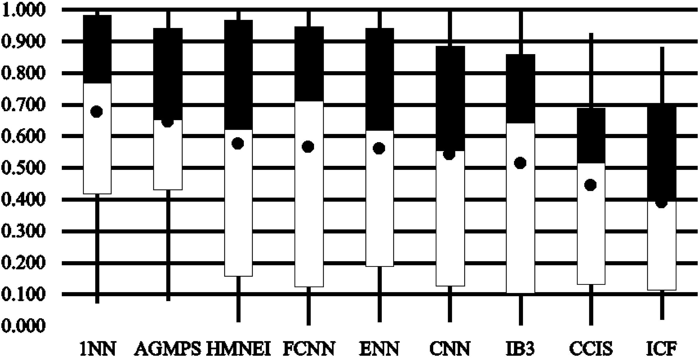

5.2 Trade-off between accuracy and reduction rate

As the AGMPS method achieves the highest accuracy rate and kappa value, we also compare the reduction rate and running time of AGMPS with those of other PS methods. Table 7 shows the reduction rate and the standard error sorted in descending order. The CCIS method has the highest reduction rate (95.39%) because it includes two sample removal processes: one for noise and another for samples ineffective for 1NN performance. The ICF has the second highest value because it removes samples that generalize information from other samples. The FCNN and CNN methods have the third and fourth highest values because they are condensation methods that keep only a small number of samples near the decision boundary. Although the AGMPS method has a relatively low reduction rate (71.21%), it can handle the trade-off between accuracy rate, kappa and reduction rate reasonably well as shown in Figs 5 and 6.

Table 7
Average reduction rate (%) and standard error of PS methods

PS Methods	CCIS	ICF	FCNN	CNN	IB3	AGMPS	HMNEI	ENN
Reduction rate	95.39	83.55	76.08	76.25	78.99	71.21	60.05	18.27
Standard error	0.0168	0.0285	0.0405	0.0375	0.0426	0.0209	0.0372	0.0476

Figure 5.

Graphic comparison of accuracy and reduction rate on the six largest datasets.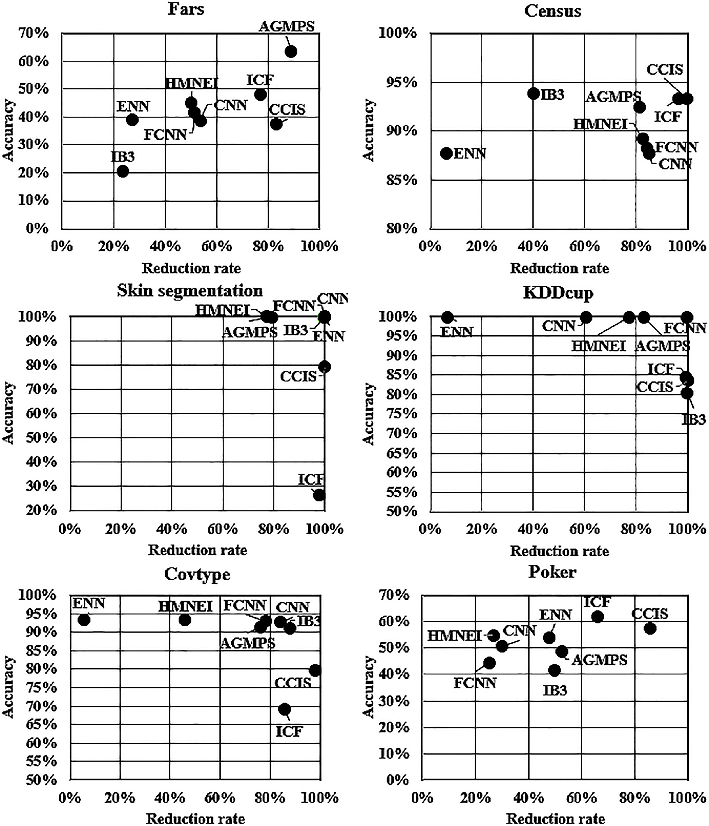

Figure 5 compares graphically the accuracy and reduction rates of AGMPS and all the PS methods considered using six large datasets: Fars, Census, Skin, KDDCup, Covtype, and Poker. The results show how effectively PS methods can handle large amounts of data. The reduction rate of the AGMPS method is slightly lower than those of the top algorithm on these datasets (except for the Poker dataset) with an 80% average reduction rate.

Figure 6 compares graphically the kappa value and reduction rate of AGMPS and all the considered PS methods considered using the six large datasets. The AGMPS method has better performance than all the other PS methods for the Fars and Census datasets. On Skin, KDDcup, and Covtype datasets, AGMPS is only slightly lower than the top right corner of ideal performance.

Figure 6.

Graphic comparison of kappa and reduction rate on the six largest datasets.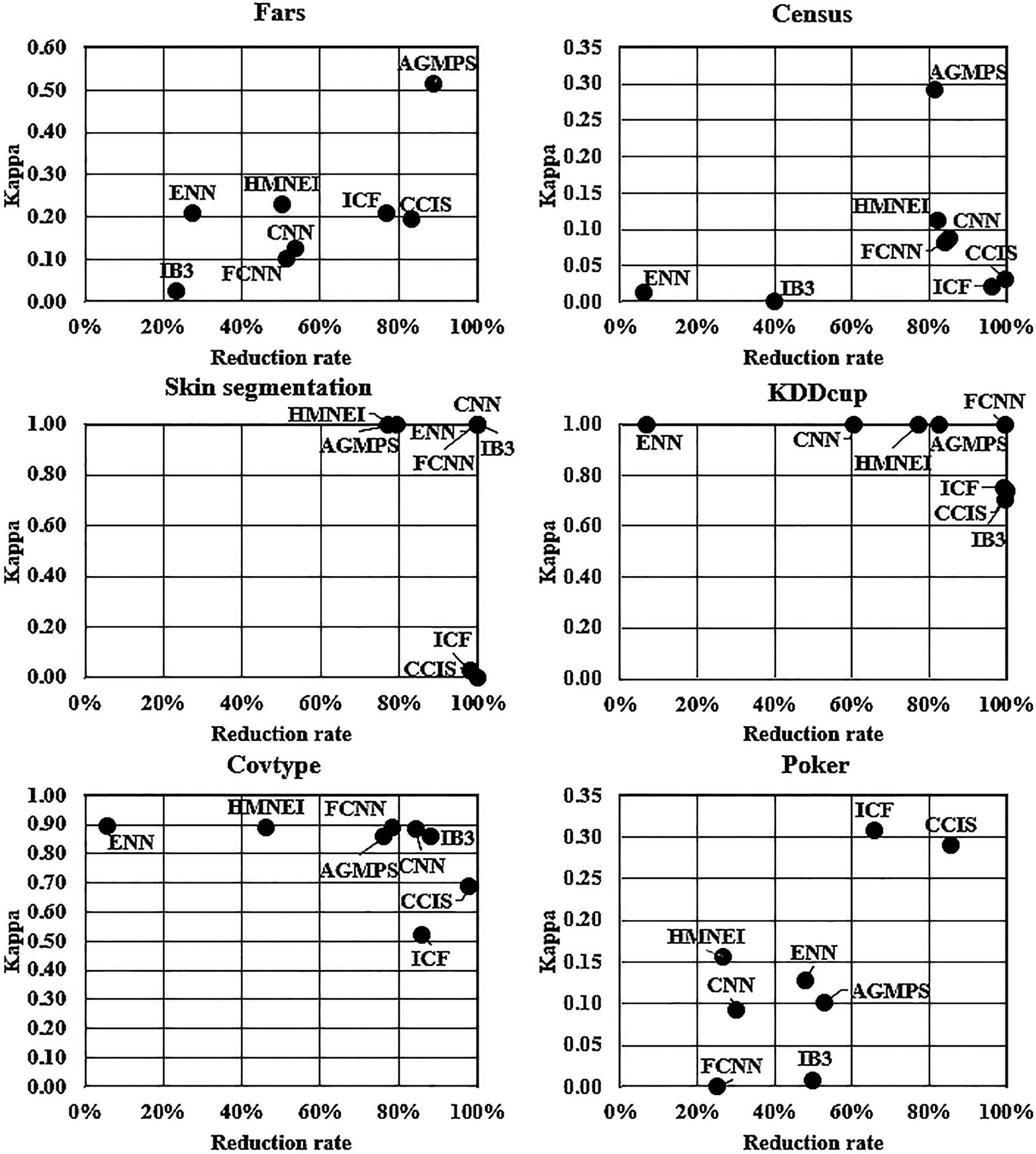

5.3 Speeding up the algorithm

The running time of the AGMPS model, the 1NN baseline model, and all considered PS methods are shown in Table 8 for the the six largest datasets because for the the smaller datasets the running times for all models were similar and the AGMPS method is the fastest.

Table 8
Running time (minutes) and speedup (times) of all methods

Dataset	1NN	AGMPS	CNN	FCNN	ENN	IB3	ICF	HMNEI	CCIS
Fars	22	14	3632	22	27	1.35	92	40	59
Skin	27	19	3	0.23	36	0.05	107	14	81
Census	72	43	1718	109	272	267	1319	147	58
KDD Cup	404	76	1864	3	479	0.75	2331	504	1044
Covertype	734	108	5934	804	881	219	2461	1293	1821
Poker	845	295	23069	2915	1421	1829	12995	7357	2709
Average	88.4	24.6	1452.0	154.4	125.2	92.8	774.3	374.7	231.6
Std. error	45.7	12.4	943.7	119.4	67.2	73.6	527.8	295.9	131.8
Speedup	1.0	3.59	0.06	0.57	0.71	0.99	0.11	0.24	0.38

Furthermore, based on a comparison of the running times of all the PS methods considered with that of the 1NN classifier in terms of speedup, Table 8 also shows that the AGMPS method is approximately 3.59 times faster than the baseline model.

5.4 Wilcoxon Rank Sum test

We measure the classification accuracy before conducting significance tests on the result of AGMPS and other PS methods. Due to the assumptions of the Wilcoxon Rank Sum test, we run Barlett’s test that tests the null hypothesis that all input samples are from populations with equal variances. Table 9 shows that the classification accuracy variance of AGMPS is not significantly different from the other PS methods, excluding IB3. Thus we cannot use the Wilcoxon Rank Sum test to compare AGMPS and IB3.

Table 9
Results of Barlett’s test for accuracy and kappa variance equality

Paired methods	Accuracy		Kappa
	$p$ -value	Result	$p$ -value	Result
AGMPS vs. CNN	0.1287	Accept $H_{0}$	0.4082	Accept $H_{0}$
AGMPS vs. FCNN	0.1229	Accept $H_{0}$	0.3221	Accept $H_{0}$
AGMPS vs. ENN	0.0641	Accept $H_{0}$	0.3325	Accept $H_{0}$
AGMPS vs. IB3	0.0311	Reject $H_{0}$	0.2927	Accept $H_{0}$
AGMPS vs. ICF	0.2255	Accept $H_{0}$	0.7651	Accept $H_{0}$
AGMPS vs. HMNEI	0.1087	Accept $H_{0}$	0.3690	Accept $H_{0}$
AGMPS vs. CCIS	0.2113	Accept $H_{0}$	0.7364	Accept $H_{0}$

We run the Wilcoxon Rank Sum test for the classification accuracy and kappa measurement, comparing the results of the AGMPS method with those of all considered PS methods at a 0.05 significance level. There are two hypotheses in these tests. The null hypothesis is $H_{0}$ : “The accuracy rate of the AGMPS method is equal to the accuracy rate of the paired algorithm”. The alternative hypothesis is $H_{1}$ : “The accuracy rate of AGMPS method is not equal to the accuracy rate of the paired algorithm”. The results in Table 10 indicate that the differences between AGMPS and the four PS methods (CNN, FCNN, ENN, and HMNEI) are not significant and therefore, we can accept $H_{0}$ (“The accuracy rate of the AGMPS method is equal to the accuracy rate of the paired algorithm”).

Table 10

Results of the Wilcoxon Rank Sum test for accuracy comparison

Paired methods	$R^{+}$	$R^{-}$	Equality		Difference
			$p$ -value	Result	$p$ -value	Result
AGMPS vs. CNN	188	137	0.5077	Accept $H_{0}$	–	–
AGMPS vs. FCNN	165	160	0.7292	Accept $H_{0}$	–	–
AGMPS vs. ENN	167	158	0.7196	Accept $H_{0}$	–	–
AGMPS vs. HMNEI	155	170	0.8532	Accept $H_{0}$	–	–
AGMPS vs. ICF	293	32	0.0011	Reject $H_{0}$	0.0008	Reject $H_{0}$
AGMPS vs. CCIS	261	64	0.0067	Reject $H_{0}$	0.0033	Reject $H_{0}$

However, the difference between AGMPS and the other two methods (ICF and CCIS) is statistically significant. When we test a one-sided Wilcoxon Rank Sum test that has $H_{0}$ : “The accuracy rate of AGMPS is equal to the accuracy rate of the paired algorithm” and $H_{1}$ : “The accuracy rate of AGMPS is greater than the accuracy rate of the paired algorithm”. Table 10 shows the results of the one-sided Wilcoxon Rank Sum test which indicate that the accuracy rate of AGMPS is significantly greater than those of ICF and CCIS methods.

First, we run Barlett’s test on the equality of variances. Second, we measure the kappa values in order to compare the results of AGMPS with the other PS methods. The results in Table 9 show that the classification kappa variance of AGMPS method is not significantly different from the other PS methods.

Table 11

Results of the Wilcoxon Rank Sum test for kappa comparisons

Paired methods	$R^{+}$	$R^{-}$	Equality		Difference
			$p$ -value	Result	$p$ -value	Result
AGMPS vs. CNN	191.5	133.5	0.4432	Accept $H_{0}$	–	–
AGMPS vs. FCNN	160.5	139.5	0.7751	Accept $H_{0}$	–	–
AGMPS vs. ENN	152.5	172.5	0.7982	Accept $H_{0}$	–	–
AGMPS vs. HMNEI	137.0	163.0	0.7210	Accept $H_{0}$	–	–
AGMPS vs. IB3	249.5	74.5	0.0185	Reject $H_{0}$	0.0092	Reject $H_{0}$
AGMPS vs. ICF	306.0	19.0	0.0001	Reject $H_{0}$	0.0001	Reject $H_{0}$
AGMPS vs. CCIS	283.0	42.0	0.0006	Reject $H_{0}$	0.0003	Reject $H_{0}$

Moreover, the result of Wilcoxon Rank Sum test for kappa measurement is shown in Table 11 at the significance level of 0.05. There are two hypotheses in these tests. The null hypothesis is $H_{0}$ : “The kappa of AGMPS is equal to the kappa of the paired algorithm”. The alternative hypothesis is $H_{1}$ : “The kappa of AGMPS is not equal to the kappa of the paired algorithm”. Table 11 shows the results of the Wilcoxon Rank Sum test for kappa measurement and indicates that the kappa differences between AGMPS and the four PS methods (CNN, FCNN, ENN, and HMNEI) are not significant.

Otherwise, the difference between AGMPS and the three other methods (IB3, ICF, and CCIS) is significant a 0.05. We also performed one-sided Wilcoxon Rank Sum test for kappa value greatness. This test has two hypotheses: $H_{0}$ : “The kappa value of AGMPS is equal to the kappa value of the paired algorithm” and $H_{1}$ : “The kappa value of AGMPS is greater than the kappa value of the paired algorithm”. In Table 11 shows that the kappa values of AGMPS are significantly greater than those of the IB3, ICF, and CCIS methods.

5.5 Noise tolerance test

We use five data sets following three different schemes to compare the classification accuracy and Cohen’s kappa of the AGMPS method with those of two edition (ENN and All-KNN) methods. First, the Noisy Train-Noisy Test scheme is the most common noise scenario because of the low-quality of the data source and the effect of the environment during the data collection process. Therefore, noise occurs in both the training data and test data simultaneously. Second, the Noisy Train-Clean Test scheme commonly can be sourced from errors in the data collection and data preparation processes. This scheme often appears when the new data are handled for the first time. Lastly, the Clean Train-Noisy Test scheme shows that the 1NN classifier model is created from the clean training data before noise occurs in the test data. The two above schemes have higher possibility of occurrence than the Clean Train-Noisy Test scheme.

Figure 7.

Graphic comparison of average accuracy and kappa on six datasets with attribute noise.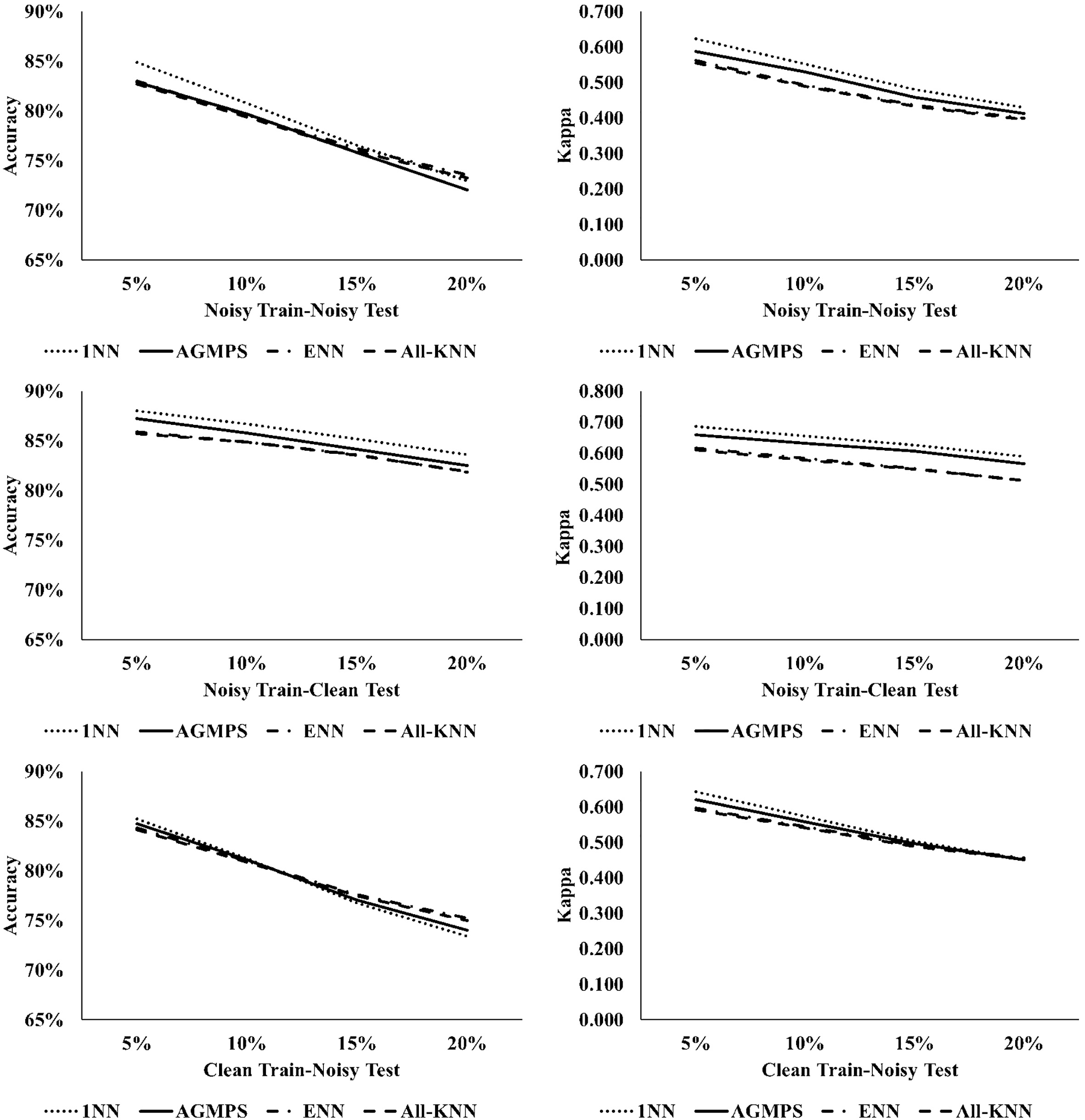

In Fig. 7, the line plots represent the trend of the accuracies and kappa values of all PS methods as well as the 1NN baseline model in the three different noise schemes. The accuracy values of the AGMPS method and the other compared methods are similar in two noise schemes (Noisy Train-Noisy Test and Noisy Train-Clean Test). The AGMPS method has a better kappa value than the ENN and All-KNN methods, where the higher line indicates that AGMPS has a higher degree of agreement between the predicted label and the actual label than the ENN and All-KNN methods in multi-class classifications.

Table 12

Results of Barlett’s test for accuracy and kappa variance equality in attribute noise test.

Paired methods	Accuracy		Kappa
	$p$ -value	Result	$p$ -value	Result
AGMPS vs. ENN	0.4408	Accept $H_{0}$	0.7648	Accept $H_{0}$
AGMPS vs. All-kNN	0.4184	Accept $H_{0}$	0.7519	Accept $H_{0}$

Table 13

Results of the Wilcoxon Rank Sum test for accuracy comparison in attribute noise test

Paired methods	$R^{+}$	$R^{-}$	Equality		Difference
			$p$ -value	Result	$p$ -value	Result
AGMPS vs. ENN	13	65	0.0413	Reject $H_{0}$	0.02068	Reject $H_{0}$
AGMPS vs. All-kNN	17	61	0.0836	Accept $H_{0}$	–	–

We run Barlett’s test for the null hypothesis that all input samples are from populations with equal variances. Table 12 shows that the classification accuracy and kappa variance of AGMPS is not significantly different from the ENN and All-KNN methods. The results in Table 13 indicate that the classification accuracy differences between AGMPS and the All-KNN method are not significant. However, the results of the one-sided Wilcoxon Rank Sum test indicate that the accuracy rate of AGMPS method is significantly less than that of the ENN method. Moreover, Table 14 shows the kappa difference between AGMPS and the two other methods (ENN and All-KNN) is significant at the 0.05 level. In addition, the kappa values of AGMPS are significantly greater than those of the ENN and All-KNN methods.

Table 14

Results of the Wilcoxon Rank Sum test for kappa comparison in attribute noise test

Paired methods	$R^{+}$	$R^{-}$	Equality		Difference
			$p$ -value	Result	$p$ -value	Result
AGMPS vs. ENN	71	7	0.0121	Reject $H_{0}$	0.0060	Reject $H_{0}$
AGMPS vs. All-kNN	74	4	0.0059	Reject $H_{0}$	0.0029	Reject $H_{0}$

6. Conclusion

This paper proposes an extended prototype selection approach based on the Geometric Median (GM). This approach focuses on speeding up the overall processing time while still providing a comparable reduction rate and classification accuracy. The process of building the classifier model is the most time-consuming part when large amounts of training data are processed. To speed up this process, we partition the data into independent subsets and process the data in each partition separately. The AGMPS method is designed to select a class representative in each disjoint partition. There are two main processes to the AGMPS method. First, the Appropriate Partition Size Assignment (APSA) process calculates the optimal number of partitions by finding a root of the derivative based on the average distance of the GM. Second, the geometric median prototype selection (GMPS) process selects a subset of class representatives from the dataset. Both processes calculate and select a prototype from a subset of samples in each partition. Therefore, this does not require the entire dataset to be loaded into memory. Furthermore, the time complexity of each process is linear. This speed of data partitioning process means that the method scales well when applied to processing large quantities of data.

The results of this experiment show that speed is the main strength of our method. The running time of our AGMPS method is much shorter than that of all other PS methods studied because the AGMPS method does not require complex computations such as finding nearest neighbors in the whole dataset or finding samples close to decision boundaries. The AGMPS method provides classification accuracy and kappa values that are comparable to those of four state-of-the-art PS methods (CNN, FCNN, ENN, and HMNEI). When compared with IB3, AGMPS is significantly more accurate based on Cohen’s kappa. In addition, the classification accuracy and kappa of AGMPS are significantly better than those of the ICF and CCIS methods which have the top two highest reduction rates in this experiment.

Finally, the results of our tests on a variety of datasets confirm the initial premise of the effectiveness of the proposed method for improving the running time of kNN algorithms with comparable reduction rate and classification accuracy.

In future work, the AGMPS method will be applied in a parallel and distributed processing system. This work should improve the processing speed of the AGMPS method. Furthermore, we aim to continue to reduce the issues associated with processing handling real-world big datasets with AGMPS. This research will show the scalability of AGMPS on the Big Data problem.

Footnotes

Acknowledgments

This work was financially supported by the Department of Computer Science and was partially supported by a grant from the Faculty of Science, Kasetsart University, Bangkok, Thailand. The authors thank Dr. Miro Lehtonen for providing many useful comments.

References

Ben-David

, A lot of randomness is hiding in accuracy, Engineering Applications of Artificial Intelligence 20 (2007), 875–885.

Kasemtaweechok

and Suwannik

, Prototype selection for k-nearest neighbors classification using geometric median, in: the Fifth International Conference on Network, Communication and Computing, ACM, Kyoto, 2016, pp. 140–144.

Nettleton

Orriols-Puig

and Fornell

, A study of the effect of different types of noise on the precision of supervised learning techniques, Artificial Intelligence Review 33 (2010), 275–306.

Wilson

D.L.

, Asymptotic properties of nearest neighbor rules using edited data, IEEE Transactions on Systems, Man, and Cybernetics: Systems SMC-2 (1972), 408–421.

Wilson

D.R.

and Martinez

T.R.

, Reduction techniques for instance-based learning algorithms, Machine Learning Journal 38 (2000), 257–286.

Hochbaum

D.S.

, Greedy strikes back: Heuristics for the fixed cost median problem, Mathematical Programming 22 (1982), 148–162.

Aha

D.W.

Kibler

and Albert

M.K.

, Instance-based learning algorithms, Machine Learning Journal 6 (1991), 37–66.

Marchiori

, Hit miss networks with applications to instance selection, Journal of Machine Learning Research 9 (2008), 997–1017.

Marchiori

, Class conditional nearest neighbor for large margin instance selection, IEEE Transactions on Pattern Analysis and Machine Intelligence 32 (2010), 364–370.

10.

Angiulli

, Fast nearest neighbor condensation for large data sets classification, IEEE Transactions on Knowledge and Data Engineering 19 (2007), 1450–1464.

11.

Wilcoxon

, Individual comparisons by ranking methods, Biometrics Bulletin 1 (1945), 80–83.

12.

Gates

G.W.

, The reduced nearest neighbor rule, IEEE Transactions on Information Theory 18 (1972), 431–433.

13.

Brighton

and Mellish

, Advances in instance selection for instance-based, Data Mining and Knowledge Discovery Journal 6 (2002), 153–172.

14.

Tomek

, An experiment with the edited nearest-neighbor rule, IEEE Transactions on Systems, Man, and Cybernetics: Systems SMC-6 (1976), 448–452.

15.

Alcala-Fdez

Fernandez

Luengo

Derrac

Garcia

Sanchez

and Herrera

, KEEL data-mining software tool: Data set repository, integration of algorithms and experimental analysis framework, Journal of Multiple-Valued Logic and Soft Computing 17 (2011), 255–287.

16.

Olvera-Lopez

J.A.

Carrasco-Ochoa

J.A.

and Martinez Trinidad

J.F.

, A review of instance selection methods, Artificial Intelligence Review 34 (2010), 133–143.

17.

Sanchez

J.S.

Pla

and Ferri

, Prototype selection for the nearest neighbour rule through proximity graphs, Pattern Recognition Letter 18 (1997), 507–513.

18.

Sanchez

J.S.

, High training set size reduction by space partitioning and prototype abstraction, The Journal of the Pattern Recognition Society 37 (2004), 1561–1564.

19.

Ingber

, Simulated annealing: Practice versus theory, Mathematical and Computer Modelling 18 (1993), 29–57.

20.

Lichman

, UCI Machine Learning Repository, http://archive.ics.uci.edu/ml, University of California, 2013.

21.

Lozano

Sotoca

Sanchez

J.S.

Pla

Pekalska

and Duin

R.P.W.

, Experimental study on prototype optimisation algorithms for prototype-based classification in vector spaces, The Journal of the Pattern Recognition Society 39 (2006), 1827–1838.

22.

Bartlett

M.S.

, Properties of Sufficiency and Statistical Tests, in: The Royal Society of London Series A Mathematical, Physical and Engineering Sciences, The Royal Society Publishing, London, 1937, pp. 268–282.

23.

Megiddo

and Tamir

, On the complexity of locating linear facilities in the plane, Operations Research Letters 1 (1982), 194–197.

24.

Altman

N.S.

, An introduction to kernel and nearest neighbor nonparametric regression, The American Statistician 46 (1992), 175–185.

25.

Hart

P.E.

, Greedy Strikes Back: The Condensed Nearest Neighbor Rule, IEEE Transactions on Information Theory 14 (1968), 515–516.

26.

Bradley

P.S.

Mangasarian

O.L.

and Street

W.N.

, Clustering via concave minimization, in: Advances Neural Information Processing Systems, MIT PRESS, Denver, 1996, pp. 368–374.

27.

Silva

R.S.

Gomes

G.M.C.

Alvim

M.S.

and Goncalves

M.A.

, Compression-based selective sampling for learning to rank, in: 25th ACM International on Conference on Information and Knowledge Management, ACM, Indianapolis, 2016, pp. 247–256.

28.

Garcia

Derrac

Cano

J.R.

and Herrera

, Prototype selection for nearest neighbor classification: Taxonomy and empirical study, IEEE Transactions on Pattern Analysis and Machine Intelligence 34 (2012), 417–435.

29.

Guha

and Khuller

, Greedy strikes back: improved facility location algorithms, Journal of Algorithm 31 (1999), 228–248.

30.

Kirkpatrick

Gelatt

C.D.

, Jr. and Vecchi

M.P.

, Optimization by simulated annealing, SCIENCE 220 (1983), 671–680.

31.

, A 1.488 Approximation algorithm for the uncapacitated facility location problem, Information and Computation 222 (2013), 45–58.

32.

Cover

T.M.

and Hart

P.E.

, Nearest neighbor pattern classification, IEEE Transactions on Information Theory 13 (1967), 21–27.

33.

Yamane

, Statistics: An Introductory Analysis, Book, Harper and Row, New York, 1967.

34.

Zhang

Ramakrishnan

G.R.

and Livny

, BIRCH: An efficient data clustering method for very large databases, in: ACM SIGMOD international conference on Management of data, ACM, Montreal, 1996, pp. 103–114.

35.

Zhu

and Wu

, Class noise vs. attribute noise: a quantitative study, Artificial Intelligence Review 22 (2004), 177–210.

Adaptive geometric median prototype selection method for k-nearest neighbors classification

Abstract

Keywords

1. Introduction

2. Related work

3. Adaptive geometric median prototype selection (AGMPS)

3.4 Noise and missing values

4. Experimental materials and methods

Table 1 State-of-the-art PS methods considered in this study

Table 3 Description of dataset

5. Results

5.1 Classification performance

Table 5 Accuracy (%) and standard error of 1NN, AGMPS, and other PS methods

Table 7 Average reduction rate (%) and standard error of PS methods

Table 8 Running time (minutes) and speedup (times) of all methods

Table 9 Results of Barlett’s test for accuracy and kappa variance equality

Footnotes

Acknowledgments

References

Table 1
State-of-the-art PS methods considered in this study

Table 3
Description of dataset

Table 5
Accuracy (%) and standard error of 1NN, AGMPS, and other PS methods

Table 7
Average reduction rate (%) and standard error of PS methods

Table 8
Running time (minutes) and speedup (times) of all methods

Table 9
Results of Barlett’s test for accuracy and kappa variance equality