Facing the full model selection problem in high volume datasets employing intelligent proxy models

Abstract

Full model selection is a technique to improve the accuracy of machine learning algorithms through the search of the most appropriate combination on each dataset of feature selection, data preparation, a learning algorithm and the adjustment of its hyper-parameters. This paradigm has been widely studied in datasets of moderate size, but poorly explored in high volume datasets. One of the main reasons is the high search space and an elevated number of fitness evaluations of candidate models. In order to overcome this obstacle, the use of proxy models or surrogate functions has been proposed in the literature. In this work, we propose the use of the full model selection paradigm to construct proxy models. Such proxy models were employed to assist in the search of models in high volume datasets in order to reduce the number of fitness evaluations and to guide the search. The obtained results, show a performance without significant differences in comparison to the complete search algorithm, using just the third part of the expensive fitness evaluations.

Keywords

Proxy models model selection big datasets

1. Introduction

The development and the low cost of new technologies have made it possible to generate large amounts of information, just in 2014, 2.5 quintillions of Bytes were daily created. This means that 90% of the data in the world was created in an interval of two years [29]. This information can become a valuable asset through its analysis and one of the main trends to perform such analysis is with machine learning techniques. Choosing an appropriate classification algorithm is not a trivial task. This process requires to find the combination of algorithms together with its hyper-parameters to achieve the lowest misclassification rate in a large search space [27]. Other factors that have a big impact on the generalization capabilities of a classification algorithm are feature selection and data-preparation. These factors, in combination with the selection of a classification algorithm and its hyper-parameters, integrate the full model selection (FMS) paradigm. Under this paradigm, every factor combination (data-preparation technique, feature selection and a machine learning algorithm with a specific value of its hyper-parameters) represent a set of data transformations and performing the learning process over the training set [10]. The FMS analysis is not just useful to search the best learning algorithm to a dataset, also it can provide information as fittest feature-selection algorithm and number of relevant features, the fittest combination of data-preparation techniques, among others. Due to its vast search space and longer computing-times, the FMS analysis is not the first option when bigger datasets are analyzed. In order to explore how to face this problem in high-volume datasets, this work proposes the use of proxy models created through the use of the FMS paradigm. This work is organized as follows: in Section 2 the related works are analyzed, Section 3 provides information about the MapReduce programming model and the Big Data paradigm. In Section 4 a definition of the FMS problem is given, Section 5 describes our proposed approach. In Section 6 are the experiments and Section 7 is for the conclusions.

2. Related works

In this section, the relevant works to our approach are presented. The full model selection problem has been addressed as an optimization one, varying the search technique employed. Escalante et al. defined the full model selection problem [10]. It was faced with the use of a particle swarm optimization algorithm (PSO), while Bansal and Sahoo used an algorithm inspired by the behavior of bats (bat algorithm) [2]. In the case of evolutionary algorithms, Chatelain et al. presented a method for model selection based on a multi-objective genetic algorithm where, the evaluation function took into account sensitivity as well as specificity and, in order to define the set of preferred solutions, the Pareto optimality principle was employed [4]. On the other hand, Rosales-Pérez et al. addressed the search phase with a multi-objective genetic algorithm. They took into account misclassification rate and, the complexity of models, computed through the Vapnik-Chervonenkis dimension (VC) [23]. As it can be seen, the search process needs to explore a large number of potential models, which implies a series of learning processes and data transformations. These factors joined to dataset size increase the computing time employed in the search of models. Similar problems where the computing time is prohibitive, have been approached in literature through the use of proxy models also known as surrogate functions. A proxy model is a computationally inexpensive alternative to a full numerical simulation and can be defined as mathematically, statistically, or data-driven model that replicates the simulation model output for selected input parameters [1]. The main approaches analyzed, relevant to this work can be grouped in the next categories (in this work we will employ the terms proxy models, surrogate functions and surrogate models).

The surrogate function is based on a single regression algorithm to predict the fitness in the objective or objectives to optimize [7, 20, 22]. Cruz-Vega et al. employed a neural network based on fuzzy granules [7]. The granules were updated periodically and evaluated by a fuzzy fitness function in order to determine if a granule must be removed or not. Pavelski et al. employed an ELM algorithm (Extreme Learning Machines) as a surrogate function and, it was optimized using the SUMO (Surrogate Modelling) framework of Matlab [20]. Rosales-Pérez et al. proposed the use of a multi-objective genetic algorithm assisted by surrogate functions for model selection [22]. Neural networks with their hyper-parameters previously selected were employed to predict each objective. Each generation of the GA, the proxy models predicted the performance in each objective of the individuals and, those considered as promising according to their expected fitness were evaluated with the time-consuming fitness function, the rest were discarded. On these works, just one kind of regression algorithm was contemplated for the construction of surrogate models. Just in [7, 20], update and hyper-parameter optimization of the employed surrogate models were taken into account. Despite the advantages of these works, it can not be determined in advance that an algorithm is the most suitable for the construction of surrogate models in a wide range of problems or during all generations in an evolutionary algorithm.

Model selection is employed in order to increase the quality of surrogate functions [5, 6, 14, 21]. An island model genetic algorithm was employed by Couckuyt et al. for model selection and hyper-parameter optimization of the proxy models [5]. The GA was combined with the Expected Improvement algorithm (EI) for the selection of data points to improve the performance of the proxy models. Crombecq et al. employed the SUMO framework for hyper-parameter optimization combined with several methods of sequential design for the construction of surrogate models [6]. Gorissen et al. employed an island model GA for model selection and hyper-parameter optimization combined with several sampling methods for the selection of data points in the construction of proxy models [14]. Pilat and Neruda performed model selection among several algorithms with their hyper-parameters previously configured by hand [21]. In all these works, the importance of model selection and hyper-parameter optimization is emphasized. It is worth to mention that in [5, 6, 14], the mechanism to create surrogate models are focused on specific problems but, these approaches could not be appropriated for the full model selection problem where surrogate models are relevant just for the dataset under analysis. Therefore, time employed in the creation of surrogate models could be employed in the search of models for the dataset under analysis.

The surrogate model is improved through instance selection [1, 12, 25, 28, 31]. Alenezi and Mohaghegh employed instance selection to build surrogate models [1]. The instances were sorted by their target value and they were over-sampled or under-sampled according to their number of occurrences. Golzari et al. employed a neural network as a surrogate function [12]. Cross-validation was used in order to compute variance prediction among several neural network models and, those instances with the biggest variance were selected to construct the final surrogate model. Pseudo-Markov chains were employed by Sundar and Shields with the purpose to select those instances near to fail domain to replicate the original fitness function [25]. Vincenzi and Gambarelli employed the Response Surface algorithm RS as a surrogate model and, a fitness measure was proposed combining the surrogate fitness and distances of the evaluated sample to the others samples as a weighted sum [28]. Yu and Wilkinson employed Genetic Programming (GP) for the creation of several surrogate models and, a GA was employed to select instances that were used to create the meta-training set [31]. In a similar way to the previous approaches, the analyzed works are not suitable for the full model selection problem because they require to invest a considerable amount of time in the construction of surrogate models instead of using this time in the search of the best model for a dataset. On the other hand, for a new dataset under analysis, there is no information in advance to build such proxy models.

As can be seen, the full model selection problem could be benefited by the use of surrogate models to reduce the high number of fitness evaluations during the search step. It is also important to mention that the amount of available information, benefits the creation of more accurate machine learning models but, the bigger the amount of data, the more computing time employed in the search. In this work, we propose the use of the algorithm PSMS (Particle Swarm Model Selection) presented in Escalante et al. but based on the MapReduce programming paradigm in order to face any dataset size. This algorithm is assisted by surrogate models selected using the full model selection approach in order to obtain adaptively, the best surrogate models during the iterations of the search step. We also propose the use of classification algorithms as surrogate models. To the best of our knowledge, this is the first work that proposes the use of the FMS paradigm and classification algorithms to build proxy models. The use of classification algorithms to create proxy models may not fit the definition of surrogate models, however, these algorithms fit better in the FMS paradigm.

3. MapReduce and high volume datasets

In this section we present some antecedents about the MapReduce programming model, the standard framework for development of Big Data analysis applications and also about the datasets of this field. MapReduce was introduced by Dean and Ghemawat in 2008 with the goal of enabling parallelization and distribution of big scale computation required to analyze large datasets [8]. This programming model was designed to work over computing clusters and it works under the master-slave communication model. The master is responsible for scheduling the jobs on the worker nodes and, the worker nodes execute tasks as directed by the master. The design of MapReduce considers the following fundamental principles:

•
Low-Cost Unreliable Commodity Hardware. The MapReduce framework is designed to run on large clusters of commodity hardware.
•
Extremely Scalable Cluster. A MapReduce node uses its own local hard drive. These nodes can be taken out of service with almost no impact to keep the MapReduce jobs running.
•
Fault tolerant. The MapReduce framework applies straightforward mechanisms to replicate data and launches backup tasks in order to keep processes running in case of failures.

In the MapReduce programming model a computing task is specified as a sequence of stages: map, shuffle and reduce that works on a dataset $X=\{x_{1},x_{2},\ldots,x_{n}\}$ . The map step applies a function $\mu$ to each value $x_{i}$ to produce a finite set of key-value pairs $(k,v)$ . To allow for parallel execution, the computation of function $\mu(x_{i})$ , must depend only on $x_{i}$ . The shuffle step collects all the key-value pairs produced in the previous map step, and produces a set of lists, $L_{k}=(k;v_{1},v_{2},\ldots,v_{n})$ where each of such lists consists of all values $v_{i}$ , such that $k_{i}=k$ for a key $k$ assigned in the map step. The reduce stage applies a function $\rho$ to each list $L_{k}=(k;v_{1},v_{2},\ldots,v_{n})$ , created during the shuffle step, to produce a set of values $y_{1},y_{2},\ldots,y_{n}$ . The reduce function $\rho$ is defined to work sequentially on $L_{k}$ but should be independent of other lists $L_{k}$ , where $k^{\prime}\neq k$ [13]. Figure 1 shows a representation of the map, shuffle and reduce stages on a dataset represented by textures (for an easier visual interpretation).

Figure 1.
The MapReduce programming model: map, shuffle, and reduce.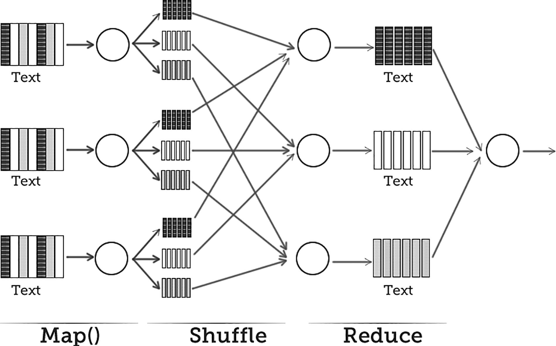

As stated earlier, the MapReduce programming model was a consequence of the emergence of the Big Data paradigm. Such paradigm refers to data objects that are too big to be processed by conventional hardware and software. An extended definition of Big Data describes this concept in terms of three characteristics of information: Volume, Velocity and Variety. Volume relates to huge quantities of data for analysis, velocity represents the frequency at which data is generated, captured and shared. Finally, variety indicates that information can be found in different formats such as text, images, audio, and video [9]. Subsequently, other Vs were added as Validity and Volatility, the first one is related to the correctness and accuracy of data regarding the intended usage. Volatility refers to the time the information is retained, because if the information is no longer useful (information about a product that is no longer sold), storage and security may become expensive to implement [16]. Despite this definition, there are no rules to identify a dataset that belongs to the Big Data paradigm and the justification of using a dataset in literature only considers its size. The size of a dataset is relative to resources available to manage such data and, in a country like Mexico (where this work was done), the availability of specialized hardware is an important limitation. Taking these factors into account, we propose an alternative definition of high volume datasets relative to the FMS problem. For our definition we propose that a high volume dataset for model selection problem must comply with two rules: 1) The dataset size is big enough so that at least one classification algorithm considered in its sequential version cannot process it. 2) The dataset size is defined by its file size considering a number of instances (I) and features (F) as long as I $\gg$ F.
4. Full model selection

As mentioned above, full model selection is the combination of several factors in order to obtain lowest misclassification rate in the dataset under analysis. These factors are feature selection, data preparation, and the selection of a learning algorithm with its hyper-parameters tuned [10]. Equation (4) is provided as formal definition. Given a set of learning algorithms $A$ , data preparation techniques $P$ and feature selection algorithms $F$ , the goal of the FMS analysis is to determine the combination of algorithms: $a^{*}_{wA}\in A$ (a machine learning algorithm with a specific configuration in its hyper-parameter values), $p^{*}\in P$ and $f^{*}\in F$ with the lowest misclassification rate. The misclassification rate is calculated on dataset $D$ and this dataset is split in two disjoint partitions ( $D^{(i)}_{\textit{train}}$ and $D^{(i)}_{\textit{validation}}$ for $i=1,2,\ldots,k$ ). The misclassification rate is calculated with the loss function $\frac{1}{k}\sum_{i=1}^{k}\mathcal{L}(a_{wA},p,f,D^{(i)}_{\textit{train}},D^{(i% )}_{\textit{validation}})$ , training the algorithm $a_{wA}$ in the partition $D^{(i)}_{\textit{train}}$ , and evaluated in the partition $D^{(i)}_{\textit{validation}}$ . The data partitions are previously transformed by $p$ and $f$ .

$\displaystyle a^{*}_{wA},p^{*},f^{*}\in\textit{argmin}\frac{1}{k}\sum_{i=1}^{k% }\mathcal{L}\left(a_{wA},p,f,D^{(i)}_{\textit{train}},D^{(i)}_{\textit{% validation}}\right)$

(1) $\displaystyle a^{(i)}\in A,p^{(i)}\in P,f^{(i)}\in F,w_{A}\in W_{A}$

Where:

$A=$ Set of available learning algorithms $P=$ Set of available data-preparation algorithms including $\varnothing$ $F=$ Set of available feature selection algorithms including $\varnothing$ $W_{A}=$ Set of hyperparameters of a learning algorithm $a$ $D_{\textit{train}},D_{\textit{val}}=$ Disjoint partitions of the dataset under analysis $\mathcal{L}=$ Loss function calculated on the validation set (misclassification rate) $\textit{argmin}=$ Values that obtains the lowest misclassification rate on the loss function $\mathcal{L}$
5. An algorithm based on MapReduce to perform FMS on high volume datasets

One of the most popular and successful algorithms to perform the FMS analysis is the Particle Swarm Model Selection (PSMS) proposed by Escalante et al. PSMS is based on the PSO algorithm, which is a population-based search inspired by the behavior of biological communities that exhibit both individual and social behavior [10]. PSMS is faster and easier to implement because it is based on a single operator as opposed to evolutionary algorithms. These algorithms require different types of operators for crossover and mutation, depending on the type of codification used in several parts that make up an individual. Due to aforementioned reasons, PSMS was chosen and adapted to the MapReduce paradigm to deal with high volume datasets.

5.1 Codification and functioning

The solutions in PSMS need to be codified in a vector called particle. Each particle $x^{t}_{i}=[x^{t}_{i,1},\linebreak x^{t}_{i,2},\ldots,x^{t}_{i,16},]$ is encoded as follows: Position 1 is for the fitness of potential models. Position 2 allows to determine which operation will be done first: data-preparation or feature selection. Position 3 indicates if data-preparation step will be done. Positions 4 to 6 are parameters for data-preparation step (method identifier, parameter 1 and parameter 2). Position 7 determines if the feature selection step will be done. Positions 8 and 9 are for the feature selection step (Method identifier and number of features to be selected respectively). Positions 10 to 16 are for the machine learning algorithm construction. As the available algorithms for feature selection, data-preparation and machine learning are different from those employed in the original work, the ranges of values that each part of a particle can take in our version of PSMS, are adjusted to the algorithms employed in this work (see Table 1). The range of values that each element in the vector can take is as follows: [0–100]; [0, 1], [0, 1], [1, 30], [1, NF], [1, 50], [0, 1], [1, 5], [1, NF], [1, 6], [1, 2], [1, 4], [1, 100], [1, 60], [1, 400], [ $-$ 20, 20] with NF $=$ Number of Features. At each time $t$ , each particle $i$ , has a position in the search space. A set of particles $S=\{x^{t}_{1},x^{t}_{2},\ldots,x^{t}_{m}\}$ is called a swarm. Each particle has a related velocity value that is used to explore the search space and the velocity of such particle at time $t$ is as follows $V^{t}_{i}=[v^{t}_{i,1},v^{t}_{i,2},\ldots,v^{t}_{i,16}]$ where $v^{t}_{i,k}$ is the velocity for dimension $k$ of the particle $i$ at time $t$ . The search trajectories are adjusted employing the following equations:

$\displaystyle v^{t+1}_{i,j}=W\times v^{t}_{i,j}+c1\times r1\times\left(p_{i,j}% -x^{t}_{i,j}\right)+c2\times r2\times\left(p_{g,j}-x^{t}_{i,j}\right)$ (2) $\displaystyle x^{t+1}_{i,j}=x^{t}_{i,j}+v^{t+1}_{i,j}$ (3)

From Eq. (2), $p_{i,j}$ is the value in dimension $j$ of the best solution found so far, also called personal best. $p_{g,j}$ is the value in dimension $j$ of the best particle found so far in the swarm. The constants $c1,c2\in\mathbb{R}$ are used to weight the influence of local and global best solutions. The values $r1,r2\sim U[0,1]$ introduce randomness into the search process. The inertia weight $W$ controls the impact of the past velocity of a particle over the current one, influencing the local and global exploration. As in the original paper, the inertia weight is adaptive and specified by the triplet $W=(w_{\textit{start}},w_{f},w_{\textit{end}})$ ; where $w_{\textit{start}}$ and $w_{\textit{end}}$ are the initial values of $W$ , $w_{f}$ indicates the fraction of iterations in which $W$ is decreased. $W$ is decreased by $W=W-w_{\textit{dec}}$ from the first iteration where $W=W_{\textit{start}}$ to last iteration where $W=w_{\textit{end}}$ and $w_{\textit{dec}}=\frac{w_{\textit{start}}-w_{\textit{end}}}{\textit{Number\_of% \_iterations}}$ [10].

5.2 Evaluation of particles in high volume datasets

In order to deal with datasets of any size, our version of PSMS is based on the MapReduce paradigm. The algorithm was developed under Apache Spark 1.6.0. We selected this framework because of its enhanced capacity to deal with iterative algorithms and the possibility to perform data processing in main memory (if memory capacity allows it). An analysis of the advantages of Spark over traditional MapReduce is out of the scope of this work, but we refer to [32]. The cornerstone of Apache Spark is the RDD or Resilient Distributed Dataset which is a collection of partitioned data elements that can be processed in parallel [15]. In Algorithm 5.2 a procedure to obtain an RDD from a plain text file is shown.

[h] Get the RDD[1] getRDD PathDataset, numparts RowRDD $=$ Load (PathDataset, numparts) RDDcol $=$ RowRDD.map (row $\rightarrow$ row.split (“,”)) RDDVect $=$ RDDcol.map (row $\rightarrow$ Vector (row.map (ColInR $\rightarrow$ ColInR.toDouble)))Return (RDDvVect)

[b] MapReduce based PSMS[1] PSMS TestSet, TrainSet, Nmodels, Ns swarm $=$ CreateInitialRandomSwarm () Generate initial swarm

pBest $=$ swarm Stores the best particles found so far

speed $=$ Matrix (swarm.rows, swarm.cols) (0)

evalParticle $=$ Array (swarm.rows) (1)

ModelsCount $=$ 0 Counts the number of times the function MRfitness is invoked

i $=$ 0 Iteration counter

ModelsCount $<$ Nmodels

i $\mod$ Ns $==$ 0 surrogateModel $=$ builSModel (trainingSurrogate) evalParticle $=$ surrogateModel (swarm) surrogateModel $\neq$ null evalParticle $=$ surrogateModel (swarm)

ModelsCount $=$ ModelsCount $+$ sum (evalParticle)

fitness $=$ MRfitness (swarm, evalParticle, TrainSet, labels)

swarm $=$ updatePos (swarm, speed)

pBest $=$ updatePBest (pBest, swarm)

trainingSurrogate $=$ mkTrainingSet (swarm, trainingSurrogate)

i $=$ i $+$ 1

finalModel $=$ buildFM (pBest) Builds final model using the best particles in pBest

finalFitness $=$ evalFinalModel (finalModel, TestSet)

The function getRDD is employed to obtain training and testing RDDs that are used as parameters for Algorithm 5.2 (MapReduce based PSMS). The Algorithm 5.2 except lines 8, 11 to 17 and 25 is essentially the same proposed in [10] and is also employed in full model selection for surrogate models. The lines mentioned above are employed in the creation/utilization of surrogate models during search stage and will be analyzed in Section 6. There are also another differences with the original work that will be summarized below:

•
The stopping criterion. Instead to perform certain number of iterations in PSO algorithm, the number of models evaluated with the costly fitness function (in this case, function MRfitness) will be used.
•
The final model is a weighted ensemble of all models stored in pBest (line 3).

In the function MRfitness, a set of transformations in the dataset will be performed and also the construction of a classifier, this function is analyzed in Algorithm 5.2.

[!ht] Fitness calculation[1] MRfitness swarm, TrainSet fitness $=$ Array [Double] (swarm.length) i $=$ 0; i $<$ swarm.length; i $++$ particle $=$ swarm (i) precedence $=$ particle (2) precedence $==$ 0 RDDPrep $=$ DataPrep (TrainSet, particle) RDDFS $=$ FeatSelection (RDDPrep, particle) fitness (i) $=$ Classification (RDDFS, particle) RDDFS $=$ FeatSelection (TrainSet, particle) RDDPrep $=$ DataPrep (RDDFS, particle) fitness (i) $=$ Classification (RDDPrep, particle) Return (fitness)

The processes of data preparation, feature selection and classification are described in the Algorithms 5.2 to 5.2. For greater ease of understanding the algorithms are remarked (the remarks are indicated by the symbol $\triangleright$ ).

[!ht] Data preparation[1] DataPrep DataSet, particle Return (DataSet.map (row $\rightarrow$ row.toArray.map (col $\rightarrow$ Transform (col, particle))))

[!ht] Feature selection[1] FeatSelection DataSet, particle numFeat $=$ particle (9) rankRDD $=$ DataSet.map (row $\rightarrow$ RankingCalculation (row)) reducedRDD $=$ rankRDD.map (row $\rightarrow$ getF (row, numFeat)) Return (reducedRDD)

[!ht] Classification[1] Classification DataSet, particle NumFolds $=$ 2 kFolds $=$ createFold (DataSet, NumFolds)

error $=$ kFolds.map $\{$ case (Training, Validation)

model $=$ createModel (Training, particle) PredictedTargets $=$ Validation.map (Instance $\rightarrow$ model.predict (Instance.features))

accuracy $=$ getAcc (PredictedTargets, Validation.targets) error $=$ 100-accuracy Return (error) $\}$ meanError $=$ error.sum/error.length Return (meanError)

In the same way as the original work, the mean of the balanced error rate (BER) over the 2-fold cross validation is used in order to evaluate the performance of every potential model. Different number of folds were evaluated (2, …,10) without significant differences and taking into account computing time, the choice was 2-fold cross validation. The algorithms employed in this work for the different stages of FMS are listed in Table 1.

Table 1
Data-preparation methods, feature selection algorithms and classification algorithms used in this work

Data-preparation algorithms Feature standardization

Normalization

Principal component analysis (PCA)

Shift and scale

Discretization

Feature selection algorithms Joint Mutual Information (JMI)

Minimum Redundancy Maximum Relevance (mrMR)

Interaction Capping (ICAP)

Conditional Mutual Information Maximization (CMIM)

Informative Fragments (IF)

Classification algorithms Support Vector Machine (SVM)

Logistic Regression (LR)

Multilayer Perceptron (MLP)

Decision Tree (DT)

Random Forest (RF)

Gradient-Boosted Trees (GBT)

6. PSMS for construction of proxy models

From Eq. (4) it can be seen that the search space of the FMS problem is infinite, even if restrictions are imposed on the hyper-parameter values of the model. The bio-inspired search methods have proved a high capacity to deal with this kind of problems and, particularly, PSMS has shown that is capable to solve the FMS problem. The nature of such problem makes it hard to asses its complexity which varies from linear to quadratic or higher orders depending on the combinations of the factors (the complexity of a Naïve Bayes classifier is lower than the one of a Random Forest algorithm). The fitness function in a normal execution of PSMS should be evaluated $\rho=m\times(I+1)$ times, where $m$ is the swarm size and $I$ the number of iterations. Supposing that the complexity of a model $\lambda$ consisting on learning algorithm, feature selection algorithm, and data-preparation techniques is bounded by $\lambda_{0}$ , the complexity of PSMS will be bounded by $\rho\times\lambda_{0}$ . The computing time of FMS is related to the dimensionality and size of the dataset, and when high volume datasets are analyzed, MapReduce allows to divide the load of data transformations and training of a learning algorithm among all available CPU-cores and MapReduce nodes. Although the complexity is the same ( $\lambda_{0}\times\rho$ ), the computing time is reduced to manageable levels. Even with the use of this paradigm, computing times are still high and considering the need of specialized hardware to perform the analysis, it is of great importance to make a better use of the MapReduce cluster that has been assigned to us and, if its possible, to reduce the time required for the analysis. An excellent alternative to do that is through the use of the previously analyzed proxy models. With the use of such tool, we can reduce the value of $\rho$ and, at the same time to use the proxy models as a compass to guide the search. In order to make easy to understand the use of proxy models to assist an algorithm (in this case PSMS) to search models in the FMS problem, the process will be described below with a generic example. Although the use of proxy models can be extended to every search algorithm, to avoid confusions, in our example this process is depicted with the PSO algorithm and the expensive fitness function could be thought as a generic time-consuming mathematical function.

1.
During the first $N-\textit{iterations}$ (a number determined by the user) of PSO, all the particles in the swarm are evaluated with the expensive fitness function.
2.
With all evaluated particles and its true fitness score, a meta-dataset is constructed (as fitness score is a continuous number, it is plain to see that this is a regression problem).
3.
A learning algorithm is trained in the meta-dataset and used in the next iteration of PSO. The particles are evaluated with the learning algorithm (from now on the proxy model) and according to their expected fitness, are marked as promising or not-promising (according to some threshold). The promising ones are evaluated with the expensive fitness function, the rest are discarded.
4.
All the particles evaluated with expensive fitness function are added to a separated file and, the meta-dataset is updated.
5.
Return to step 3 until termination criterion is met.

A variant of the previously described process is the one followed by several works in the literature, where the main efforts are to construct the proxy model and all subsequent evaluations are performed just with the surrogate function. In our problem, the fitness of possible solutions (particles) are just an estimate of the true fitness in the test set (the estimated error rate) calculated on the training set, that is why we can not use the proxy model to evaluate all particles in the search process. From the previous example we can extract some key factors of the process:

1.
During the search stage, particles in the swarm are in constant change from iteration to iteration and hyper-parameter values of the proxy model could be re-tuned to achieve a higher accuracy.
2.
The change of particles in the swarm during the search makes that importance of the meta-features changes too, therefore the use of feature selection algorithms it is also beneficial.
3.
The threshold to decide which particles are evaluated and which are not, cannot be defined in advance. Each dataset is a different problem and there is no information of the maximum accuracy that can be obtained in that dataset.

Figure 2.
Flow chart of M-PSMS and S-PSMS.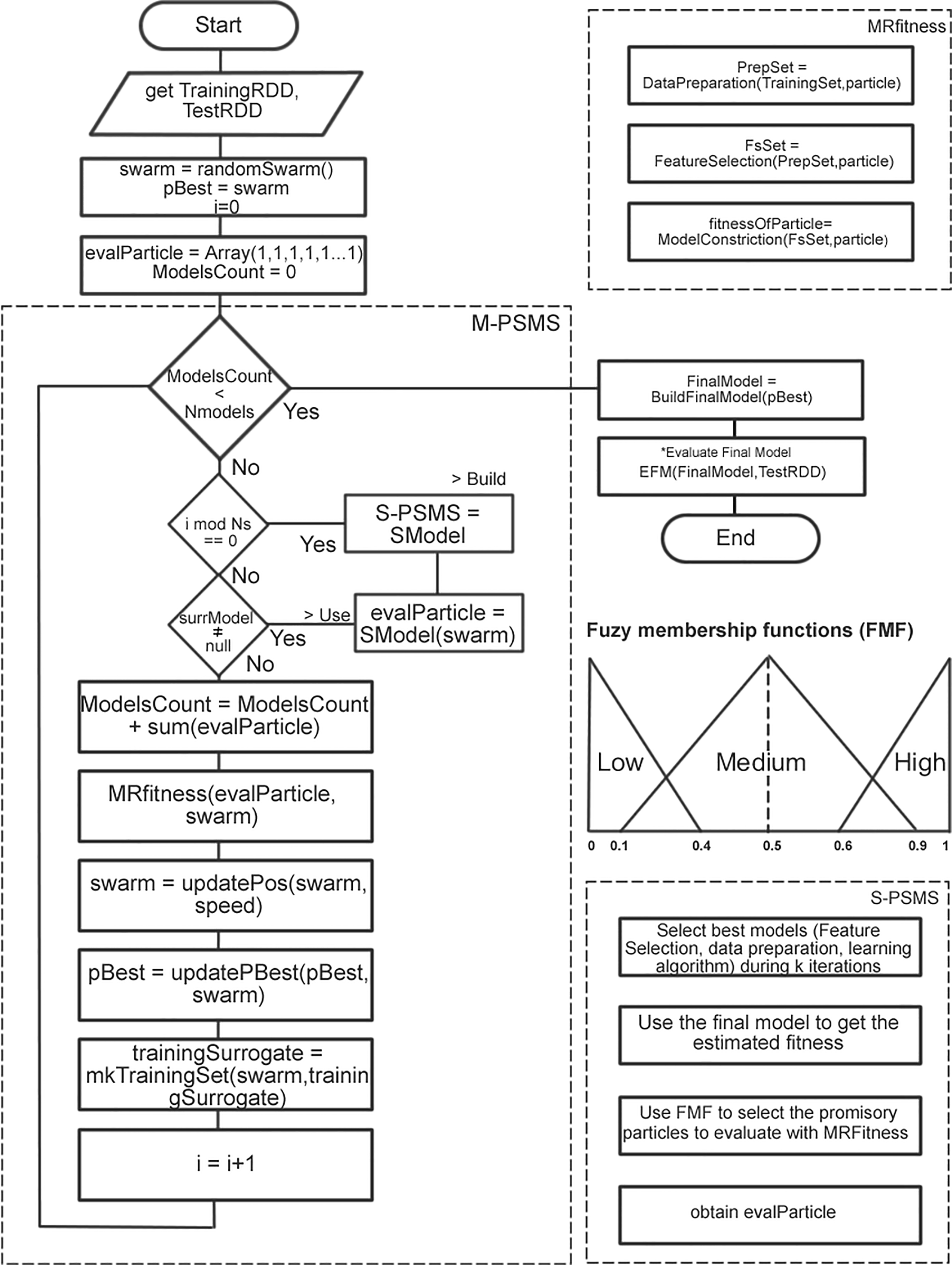

Taking into consideration all these factors, it can be seen that the FMS paradigm is well suited to construct proxy models. To understand our approach, Fig. 2 shows a flowchart and other relevant elements. Because the FMS analysis is performed to find models for high volume datasets and for proxy models construction, it is necessary to use different acronyms to differentiate both processes. With PSMS as our core algorithm to perform FMS analysis, the one used for model selection in high volume datasets from now on will be referred as M-PSMS (Main) and the one used for proxy models constructions will be referred as S-PSMS (Surrogate). In Section 5.2 it was mentioned that stopping criterion for M-PSMS is changed in order to permit the user to choose the number of models to evaluate as termination criterion instead of the number of iterations in the search algorithm. This option is very useful when the datasets to be evaluated are too big and need to use specialized hardware with a limited amount of computing time. Regarding the threshold problem, one way to solve it is through an adaptive method. With this in mind, the use of fuzzy sets was proposed. A fuzzy set is a generalization of the classical set theory. In the real world, many classes of objects are not as well defined as a regular set theory would suggest. For example, a set of all tall persons includes, of course, all persons taller than 1.9 m, but what about persons of length 1.8 m. The definition of a fuzzy set has what is needed to define a set that has inexact boundaries [17]. A fuzzy set $A^{\prime}$ in a universe of discourse $X$ is characterized by a membership function $\mu_{A^{\prime}}$ which assigns to each element $x\in X$ a real number $\mu_{A^{\prime}}(x)\in[0,1]$ expressing the membership degree of $x$ in the fuzzy set $A^{\prime}$ [26]. A membership function ( $\mu$ ) is a curve that defines how each point in the input space is mapped to a membership value.

Using fuzzy sets theory, three fuzzy membership functions (shown in Fig. 2) where created: Low, Medium and High. It was mentioned that, to measure the fitness of particles in M-PSMS was used the BER (balanced error rate), so, the particles whose BER has highest membership degree to “Low” fuzzy set, are marked as promising and the rest are discarded. As lowest BER found so far, changes from iteration to iteration of M-PSMS, it is necessary to adjust this value in every iteration to provide an adaptive mechanism to evaluate or discard the particles. It is also necessary to scale the fitness of particles in the interval [0, 1] using the maximum and minimum value of BER found so far because those limits are not known in advance.

To this point, we can say that S-PSMS is used to build proxy models instead of just re-training those proxy models. With the predicted fitness provided by S-PSMS and the use of fuzzy sets, the evalParticle vector (from line 6 of Algorithm 5.2) is used to store the labels assigned to particles and those marked with “1” are evaluated with the function MRfitness, reducing this way, the number of expensive fitness evaluations. According to the definition of proxy models and the analysis of literature provided in Section 2, the use of proxy models is faced as a regression problem, but with the addition of the fuzzy sets mechanism, this problem can be turned easily into a classification one. For this reason, we experimented with two different versions of S-PSMS, one that builds proxy models under FMS paradigm using regression algorithms (S-PSMSReg) and one with classification algorithms (S-PSMSClass). The incursion of the FMS paradigm to create proxy models comes with a series of drawbacks that were faced and are still under refinement as part of future work. That is the case of feature selection in S-PSMSReg version. Feature selection cannot be performed with traditional algorithms because as the meta-dataset represents a regression task, there are no discretized classes, which are a requirement for algorithms as FOCUS or Relief, among others. That is why in S-PSMSReg, the feature selection step is performed through the Principal Component Analysis (PCA). On the other hand, the S-PSMSClass faces discrimination of particles as a binary classification task, and at first iterations, there are more particles labeled with “0”, therefore, the problem becomes an unbalanced classification one. To overcome this problem, well-known strategies of over-sampling and under-sampling were employed in order to get an equal proportion of both classes. Finally as the creation of the proxy models through the use of the FMS paradigm takes longer time than just re-training, is necessary to provide a mechanism to control how many times this process will be performed during the execution of the M-PSMS algorithm. With this in mind, parameter $N s$ (in line 11 of Algorithm 5.2) is employed to decide during how many iterations of the M-PSMS algorithm, S-PSMS will be used until re-build the proxy model and it is set by the user.
7. Experiments and results

In the interest to evaluate the performance of the proposed algorithms, we experiment with datasets of incremental size shown in Table 2, that were obtained from UCI repository [18] and from Libsvm project [11]. The datasets “Synthetic 1” and “Synthetic 2” were created using the tool for synthetic datasets generation in the context of ordinal regression: “Synthetic Datasets Nspheres” provided in [24]. Despite having been developed for ordinal regression, the tool can be properly adjusted for traditional binary or multi-class problems and provides mechanisms to control overlaps and class balance.

Table 2
Datasets used in the experiments

Datasets	Data points	Attributes	Samples by class	Type of variables	File size
RLCP	5749111	11	(5728197; 20915)	Real	261.6 MB
KDD	4856150	41	(972780; 3883369)	Categorical	653 MB
Synthetic 1	200000000	3	(100000000; 100000000)	Real	5.5 GB
Higgs	11000000	28	(5170877; 5829123)	Real	7.5 GB
Synthetic 2	49000002	30	(24500001; 24500001)	Real	12.7 GB
Epsilon	500000	2000	(249778; 250222)	Real	15.6 GB

Another major feature of the datasets is its intrinsic dimension. The intrinsic dimension (ID) is the minimum number of parameters needed to represent data without information loss [19]. The ID of the employed datasets was estimated with the “Minimum neighbor distance estimator” (MNDE) [19] and the “Dimensionality from angle and norm concentration” (DANCO) estimator [3]. The importance of the estimation of “ID” of each dataset is to ensure that each dataset represents a different computational problem and, therefore, those proposed algorithms are capable to deal with a wide range of problems and in the context of this work also with datasets of different sizes. In Table 3, the calculated intrinsic dimension using the aforementioned estimators is shown.

Table 3

Intrinsic dimension of datasets

Datasets	MNDE	DANCO
RLCP	2	2
KDD	1	1
Synthetic 1	3	3
Higgs	12	15
Synthetic 2	22	28
Epsilon	160	78

In Section 6 it was mentioned that surrogate-assisted version of PSMS (S-PSMS) was divided into two variants, one that generates proxy models using regression algorithms (S-PSMSReg) and another that uses classification algorithms (S-PSMSClass). Both versions were contrasted to PSMS (the unassisted version) and following one of the main trends in literature, algorithms were contrasted to a search algorithm assisted by single proxy model. In our case is PSMS assisted by a Multi-layer perceptron (PSMS-MLP). In the PSMS-MLP version, the hyper-parameters of the MLP were adjusted by a grid-search at the beginning of the FMS analysis and during the rest of the process, the MLP was just re-trained with new samples of the meta-dataset. From the original work where PSMS was presented [10], the configuration values of such algorithm were obtained. The size of the swarm was increased from 5 to 30 particles and stopping criteria to perform 50 iterations was preserved. Taking these values into account, PSMS performs a search by exploring 1500 potential models (30 $\times$ 50). In Section 5.2 it was mentioned that termination criteria in the proposed approaches were changed from the number of iterations to the number of models to evaluate with the expensive fitness function (line 10 in Algorithm 5.2). In order to determine this number, fitness of all the models found with the complete search (PSMS) was stored in a vector and then, the mechanism used to determine if a particle is promising or not (from Section 6) was employed in order to know how many promising models were found in each dataset. In Table 4 these results are shown.

Table 4

Average amount of promising models found with the PSMS algorithm with a complete search of 1500 models during 20 replications in the proposed datasets

Datasets	Number of promising models
RLCP	830.70 $\pm$ 38.16
KDD	709.60 $\pm$ 192.57
Synthetic 1	404.85 $\pm$ 116.57
Higgs	508.50 $\pm$ 53.07
Synthetic 2	290.15 $\pm$ 63.53
Epsilon	310.05 $\pm$ 10.34

As the average of the reported results is of 508 potential models, termination criterion of the surrogate-assisted searches was to perform 500 evaluations with the expensive fitness function. Significance tests were performed to obtain evidence of the difference in the performance of the evaluation methods. In order to obtain a statistical power of 90% in an ANOVA test that contrasted 4 methods, 20 replications of each experiment for each dataset were performed and a Tukey test as post-hoc analysis to find significant differences (Table 6). Each replication was performed with a particular random sample of data points with different random samples among replications. For each experiment, the dataset was divided into two disjoint datasets with 60% of data samples for the training set and 40% for the test set. In Table 5 the mean classification error obtained by different algorithms in this study is shown.

Table 5

Mean classification error obtained in the test dataset by the algorithms PSMS, PSMS-MLP, S-PSMSReg and S-PSMSClass over 20 replications. The best results are in bold

Dataset	PSMS	PSMS-MLP	S-PSMSReg	S-PSMSClass
RLCP	0.052 $\pm$ 0.001	0.426 $\pm$ 1.593	0.059 $\pm$ 0.123	0.028 $\pm$ 0.067
KDD	0.156 $\pm$ 0.134	2.55 $\pm$ 7.638	0.078 $\pm$ 0.002	0.167 $\pm$ 0.147
Synthetic 1	15.86 $\pm$ 0.001	15.86 $\pm$ 0.001	15.86 $\pm$ 0.001	15.86 $\pm$ 0.001
Higgs	28.30 $\pm$ 0.006	29.49 $\pm$ 2.22	30.19 $\pm$ 0.69	28.34 $\pm$ 0.17
Synthetic 2	6.68 $\pm$ 0.001	6.68 $\pm$ 0.001	6.68 $\pm$ 0.001	6.68 $\pm$ 0.001
Epsilon	54.008 $\pm$ 0.926	32.223 $\pm$ 5.397	28.816 $\pm$ 2.762	28.232 $\pm$ 0.920

To this point, the results in Table 5 shows that S-PSMSClass obtained the best results on four of the six datasets (RLCP, Synthetic 1, Synthetic 2 and Epsilon). PSMS and S-PSMSreg obtained the best results on three datasets each one, while PSM-MLP obtained the best results just in two datasets where all contrasted methods got the same results. It is important to know that PSMS evaluates 1500 models before building the final model that was used on the test partition while all surrogate-assisted approaches (PSMS-MLP, S-PSMSReg, and S-PSMSClass) just evaluated 500 models. This means that with just the third part of the search performed by PSMS, those approaches are capable to compete with the whole search. It is also worth to note that PSMS-MLP is the approach with the highest variance in almost all datasets in contrast with the other surrogate-assisted approaches. In order to understand how the compared strategies perform the search process, the following Figs 3 and 4 show such a process on datasets Synthetic 1 and Higgs. In “X” axis is shown the average number of models evaluated as a measure of the progression of the search, and, in the “Y” axis, the estimated error of the best particle found so far ( $p_{g,j}$ ) is shown.

Figure 3.

Evolution of the search of the proposed methods in Synthetic 1 dataset. The X axis is the number of evaluated models (as a way to point out the progress of the search) and in the Y axis is the estimated error.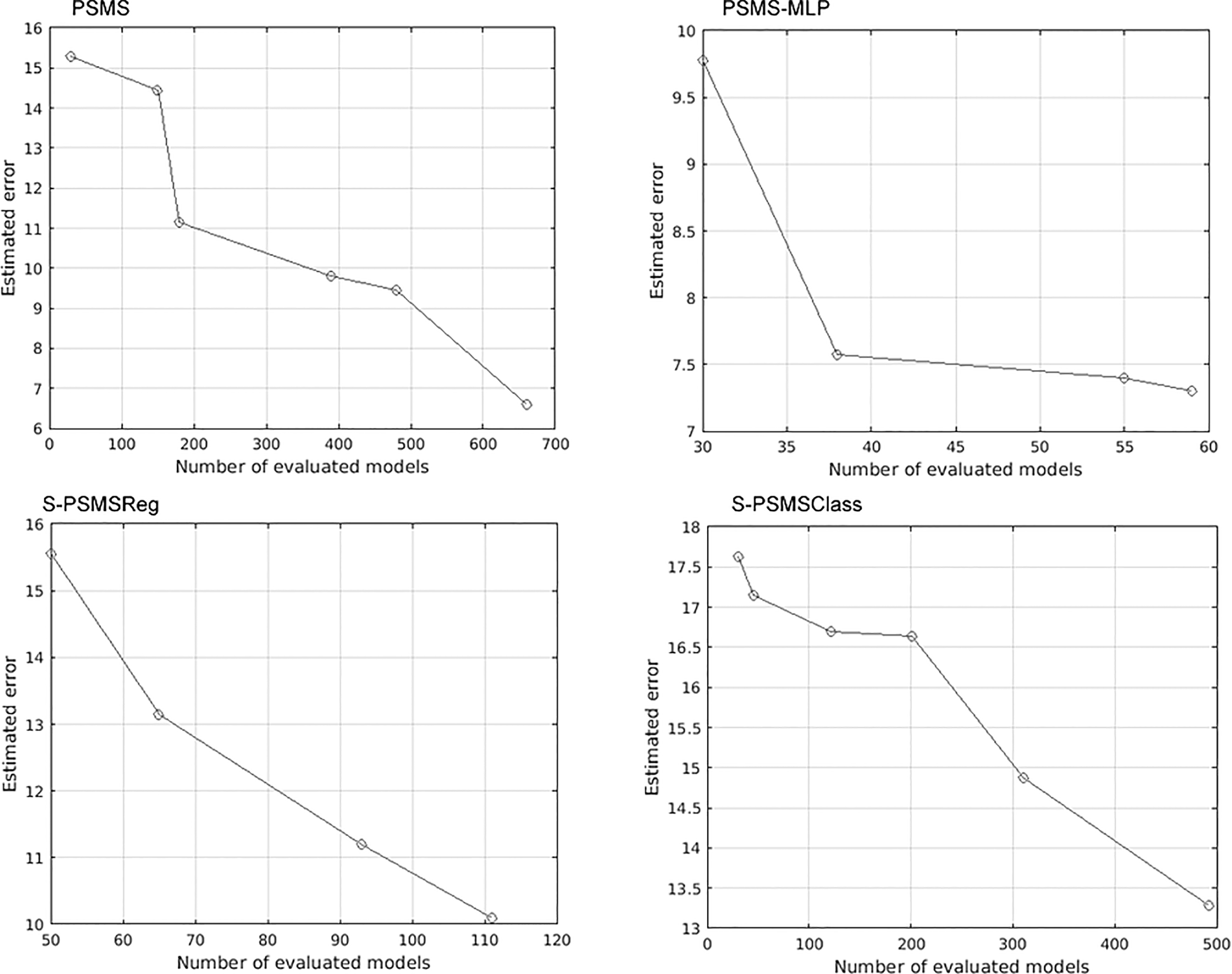

From Fig. 3, it can be seen that PSMS and PSMS-MLP obtained their estimated errors under 10% meanwhile the remaining methods obtained errors of 10 % and below 13.5%. PSMS-MLP got its lowest error early in the search with approximately 59 model evaluations in contrast with PSMS that obtained its best after 600 evaluations. The FMS based approaches obtained its best particles after 500 evaluations for S-PSMSClass and 110 evaluations for S-PSMSReg. Although all methods got the same performance on this dataset (error $=$ 15.860), it must be noted that from the proxy model based algorithms, those built under the FMS paradigm, performed a most complete search than PSMS-MLP. Despite the fact that one of the objectives on this experiment is to reduce the number of evaluated models, it is mandatory to perform a search as good as the one of PSMS or even better and employing the proxy model as a compass in order to avoid bad particles but, without circumventing entire swarms.

Figure 4.

Evolution of the search of the proposed methods in Higgs dataset. The X axis is the number of evaluated models (as a way to point out the progress of the search) and in the Y axis is the estimated error.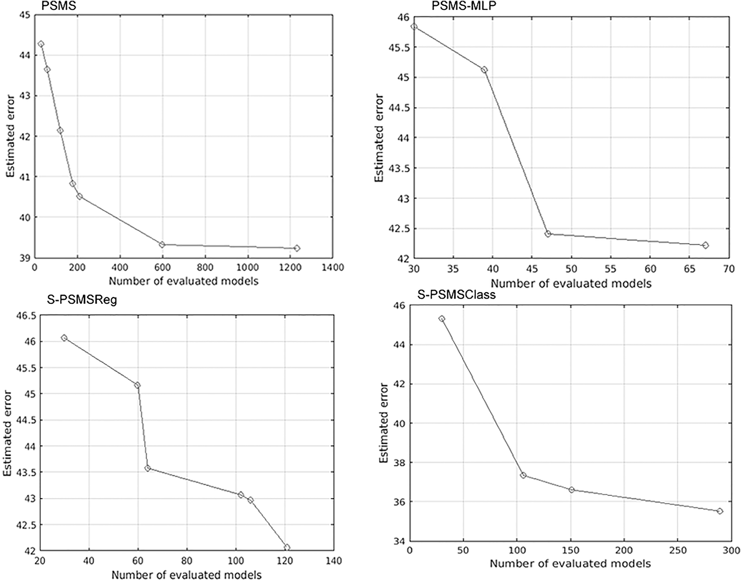

Regarding to Higgs dataset, the best performance was obtained by PSMS (error $=$ 28.3%) followed by S-PSMSClass (error $=$ 28.34%), PSMS-MLP (error $=$ 29.49%) and finally S-PSMSReg (error $=$ 30.19%). During the experimental phase of this work, termination criteria was adjusted to the approaches that use the regression algorithms (PSMS-MLP and S-PSMSReg) in order to complete 1000 iterations or to perform 500 model evaluations (whichever occurs first) because, the proxy model in both approaches becomes very selective in each iteration omitting several potential models, while the classification-based approach makes a better use of the assigned execution time. From Fig. 4, we can see that in the regression-based approaches it is common to finish the search by the criteria of reaching the maximum number of iterations. To find statistical differences among the different methods we perform an ANOVA test with 95% of confidence and the Tuckey test as a post-hoc test. In Table 6 the results are shown.

Table 6

F-statistic obtained from ANOVA test and q-values from Tukey HSD test for performing all possible pairwise comparisons among proposed strategies. The critical value at the 95% confidence level for ANOVA test is 2.72 for all datasets. The critical value at 95% confidence level for Tukey HSD test is 3.76. Cases that exceed critical value are considered as a difference that is statistically significant at the fixed level and are marked with an asterisk ( ${}^{*}$ )

Dataset	Anova F		PSMS vs PSMS-MLP		PSMS vs S-PSMSReg		PSMS vs S-PSMSClass
RLCP	1.	1323	2.	0931	0.	0412	0.	1313
KDD	2.	0111	2.	8087	0.	0912	0.	0130
Synthetic 1	1.	2341	0.	8068	1.	6136	1.	2102
Higgs	12.	626 ${}^{*}$	4.	5739 ${}^{*}$	7.	2688 ${}^{*}$	0.	1401
Synthetic 2	0.	2080	0.	4763	0.	4763	0.	4763
Epsilon	312.	307 ${}^{*}$	31.	421 ${}^{*}$	36.	335 ${}^{*}$	37.	177 ${}^{*}$

From Table 6 it can be seen that all surrogate-assisted searches had a similar performance to PSMS, exploring just a third part of the potential models (500 fitness evaluations). Although, PSMS explored more potential models, the proxy model in the other approaches has the capacity to guide the search as a compass. This situation are especially notorious in the Epsilon dataset, where all methods surpassed to PSMS and with significant differences according to Table 6. From the perspective of the “ID” analysis, we can note that this dataset is also the hardest in the comparative (dimension of 160/78). Regarding Higgs dataset, approaches with regression-based proxy models presented significant differences with respect to PSMS, despite the fact that this dataset is the third most difficult problem (ID of 12/15). Therefore, results in Tables 5 and 6 show that the best approach from the comparative is the one that does not fit the strict definition of the proxy model. S-PSMSClass not only got a performance comparable to PSMS in 5 datasets but it also surpassed the complete search in one dataset, the hardest one. Regarding the computing time factor, in Fig. 5, average execution times are shown as a bar chart in each dataset. The experiments were performed in a workstation of 12 threads with an Intel(R) Xeon(R) CPU E5-2695 at 2.40 GHz and 30 GB in RAM.

Figure 5.

Bar chart with the average execution time (in minutes) performed in 20 replications in each dataset. Each texture represent a different dataset and bars are grouped by algorithm. The standard deviation is depicted as a solid black line in the center of the bars.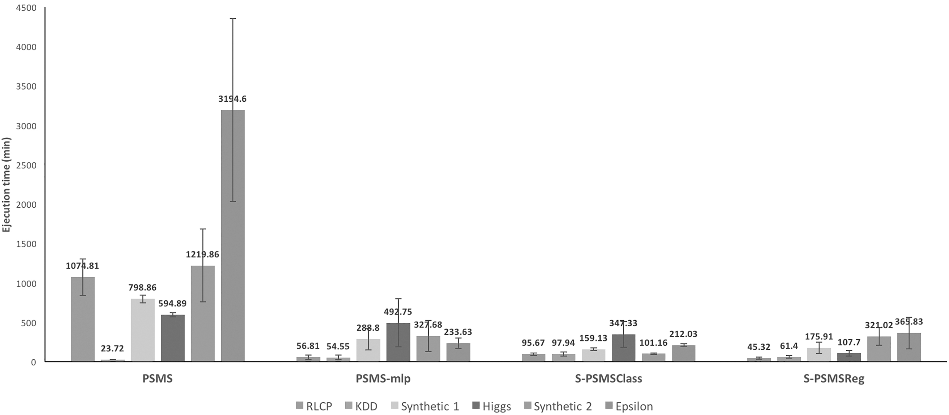

On Fig. 5, it can be appreciated the average execution times of the contrasted algorithms with the aforementioned hardware configuration. With no surprise, highest execution times are for PSMS (the complete search), while surrogate-assisted approaches are considerably faster and particularly for the Epsilon dataset. Due to its random nature (the initial swarm is randomly initialized), PSMS had also the largest standard deviation, but, taking into account that all the surrogated versions of PSMS had a random initial swarm too, we can conclude that a proxy model is capable to guide the search in an effective way. Concerning the standard deviation, a simpler visual analysis shows that proxy models constructed under the FMS paradigm had a smaller standard deviation than the traditional approach (PSMS-MLP). Finally, although computing times of S-PSMSClass were not the smallest in all datasets, results in Tables 5 and 6 and Fig. 5 shows that this non-traditional approach is capable to outperform the complete search but with moderate to low execution times. To build proxy models under the FMS paradigm and employing classification algorithms is an excellent alternative to traditional proxy models. This approach is particularly useful in problems where fitness function is just an estimation and not a true measure of the phenomenon under analysis. Although, the time-consuming construction of proxy models under the FMS paradigm could be thought as a major drawback, Fig. 5 shows that the time wasted on the construction of not promising models is considerably higher. S-PSMSClass was also contrasted against two algorithms (constructed also under the MapReduce programming model): the kernel K-NN algorithm present in [30] and a grid search that evaluated 1570 possible models. In Tables 7 and 8 mean errors obtained by the aforementioned algorithms and the significance tests are shown.

Table 7

Mean classification error obtained in the test datasets by S-PSMSClass and the obtained by K-NN (K $=$ 9,999) and Grid search, over 20 replications. The best results are in bold

Dataset	S-PSMSClass	Grid	K-NN (k $=$ 9,999)
RLCP	0.028 $\pm$ 0.067	0.001 $\pm$ 0.000	0.500 $\pm$ 0.098
KDD	0.167 $\pm$ 0.005	0.001 $\pm$ 0.000	19.535 $\pm$ 0.261
Synthetic 1	15.862 $\pm$ 0.001	17.011 $\pm$ 0.120	50.088 $\pm$ 0.028
Higgs	28.34 $\pm$ 0.17	30.955 $\pm$ 0.228	46.916 $\pm$ 0.408
Synthetic 2	6.68 $\pm$ 0.001	22.152 $\pm$ 0.541	50.126 $\pm$ 0.115
Epsilon	28.232 $\pm$ 0.920	29.664 $\pm$ 0.174	50.673 $\pm$ 3.323

Table 8

F-statistic obtained from the ANOVA test and q-values from the Tukey HSD test for performing all possible pairwise comparisons among proposed strategies. The critical value at 95% confidence level for ANOVA test is 3.16 for all datasets. The critical value at 95% confidence level for Tukey HSD test is 3.44. Cases that exceed critical value are considered as a difference that is statistically significant at fixed level and are marked with an asterisk ( ${}^{*}$ )

Dataset	Anova F		S-PSMSClass vs Grid		S-PSMSClass vs K-NN
RLCP	333.	346 ${}^{*}$	1.	772	30.	699 ${}^{*}$
KDD	83,862.	2 ${}^{*}$	4.	3024 ${}^{*}$	499.	4192 ${}^{*}$
Synthetic 1	1,479,940.	6 ${}^{*}$	71.	762 ${}^{*}$	2,142.	05 ${}^{*}$
Higgs	24,420.	67 ${}^{*}$	40.	701 ${}^{*}$	288.	715 ${}^{*}$
Synthetic 2	95,224.	53 ${}^{*}$	216.	803 ${}^{*}$	608.	822 ${}^{*}$
Epsilon	688.	937 ${}^{*}$	0.	504	45.	712 ${}^{*}$

Table 7 shows that S-PSMSClass outperformed all contrasted methods in four datasets and it was outperformed by the grid search in two (RLCP and KDD). Table 8 shows that there are significant differences in the performance of S-PSMSClass in contrast to the K-NN algorithm in all datasets, while the Grid search exceeds S-PSMSClass in the KDD dataset and there were no significant differences in the Epsilon dataset, therefore, our approach outperforms to the Grid search in 3 datasets (Synthetic 1, Higgs and Synthetic 2), was outperformed in KDD and has a similar performance to Grid search in RLCP and Epsilon. Bearing in mind that, if PSMS would have been compared against these two methods, it is more likely that it would have been surpassed by the Grid search in the Epsilon dataset. Taking into account that S-PSMSClass is a reduced search that explores only a third part of the possible models, its performance is well balanced both in terms of predictive power and execution time.

8. Conclusions and future work

The full model selection is an analysis technique capable to improve the predictive power of classification algorithms and to provide useful information about the dataset under analysis. This technique is not the first alternative when the size of a dataset is larger than usual due to high execution times. Pursuing a way to extend the FMS analysis to high volume datasets, a MapReduce based version of a well-established algorithm for FMS (PSMS) was presented. The largest computing times of such algorithm made necessary to propose alternatives to overcome this limitation and to make a better use of the budget of time for the analysis. The use of proxy models as a tool to evaluate the possible solutions (particles of a PSO search) in order to discard the non-promising ones was studied. As the proxy model could act as a compass in the search process, in order to build the best compass possible, the use of the FMS paradigm was proposed. Two main alternatives were obtained from the aforementioned approach, one using regression algorithms to replicate the behavior of the fitness function and another employing classification algorithms to discriminate the particles in two classes (promising and not promising). The searches that were assisted by the proxy models developed under the FMS paradigm were contrasted to the unassisted-search and to a search assisted by a single regression algorithm (MLP) with no hyper-parameter tunning during the search process. The experimental results show that the proposed assisted searches (S-PSMSClass and S-PSMSReg) had a similar performance to the complete search and with a smaller standard deviation compared to the search assisted by a simple regression algorithm (PSMS-MLP). The non-traditional approach (S-PSMSClass) assisted by classification-based proxy models outperformed the complete search, both in terms of predictive power and execution time. This last approach was also compared against a grid search and a K-NN algorithm (also developed under the MapReduce programming model), outperforming those methods on three datasets. To the best of our knowledge, this is the first work that proposes the use of classification algorithms in the construction of proxy models. The use of the FMS based proxy models and the use of classification algorithms are a good alternative to reduce the computing time and to guide the search process in an effective way in problems where the fitness function is just an estimate and not a real measure of the phenomenon under analysis. As future work, several aspects aimed to improve this work will be faced, the following are some of them:

•

Extend the functionality and capabilities of our approach (PSMS $+$ proxy models) to be capable to face datasets with a higher number of features than instances ( $F\gg I$ ).

•

Instance selection: Instances used in the construction of surrogate models will be selected carefully in order to improve the quality of the proxy models.

•

Quality measure: A quality measure will be proposed in order to be capable to re-use the constructed surrogate models and to reduce the time employed in their creation.

•

Better initial particles: The initial particles in the search algorithms come from a random sampling. The use of problem-specific suggestions could reduce the use of expensive fitness functions.

Footnotes

Acknowledgments

The first author is grateful for the support from CONACyT scholarship no. 428581. The authors appreciate the useful insights of Dr. Hugo Jair Escalante provided for the elaboration of this work.

References

Alenezi

and Mohaghegh

, A data-driven smart proxy model for a comprehensive reservoir simulation, in: Information Technology (Big Data Analysis) (KACSTIT), Saudi International Conference on, IEEE, 2016, pp. 1–6.

Bansal

and Sahoo

, Full model selection using bat algorithm, in: Cognitive Computing and Information Processing (CCIP), 2015 International Conference on, IEEE, 2015, pp. 1–4.

Ceruti

Bassis

Rozza

Lombardi

Casiraghi

and Campadelli

, Danco: Dimensionality from angle and norm concentration, arXiv preprint arXiv:1206.3881, 2012.

Chatelain

Adam

Lecourtier

Heutte

and Paquet

, A multi-model selection framework for unknown and/or evolutive misclassification cost problems, Pattern Recognition 43(3) (2010), 815–823.

Couckuyt

De Turck

Dhaene

and Gorissen

, Automatic surrogate model type selection during the optimization of expensive black-box problems, in: Simulation Conference (WSC), Proceedings of the 2011 Winter, IEEE, 2011, pp. 4269–4279.

Crombecq

De Tommasi

Gorissen

and Dhaene

, A novel sequential design strategy for global surrogate modeling, in: Simulation Conference (WSC), Proceedings of the 2009 Winter, IEEE, 2009, pp. 731–742.

Cruz-Vega

Alberto Reyes García

Gómez Gil

Manuel Ramírez Cortés

and de Jesús Rangel Magdaleno

, Genetic algorithms based on a granular surrogate model and fuzzy aptitude functions, in: Evolutionary Computation (CEC), 2016 IEEE Congress on, IEEE, 2016, pp. 2122–2128.

Dean

and Ghemawat

, Mapreduce: Simplified data processing on large clusters, Communications of the ACM 51(1) (2008), 107–113.

del Río

López

Benítez

J.M.

and Herrera

, On the use of mapreduce for imbalanced big data using random forest, Information Sciences 285 (2014), 112–137.

10.

Escalante

H.J.

Montes

and Sucar

L.E.

, Particle swarm model selection, Journal of Machine Learning Research 10(Feb) (2009), 405–440.

11.

Fan

, Libsvm data: Classification, regression, and multi-label, https://www.csie.ntu.edu.tw/∼cjlin/libsvmtools/datasets/, 2018.

12.

Golzari

Sefat

M.H.

and Jamshidi

, Development of an adaptive surrogate model for production optimization, Journal of Petroleum Science and Engineering 133 (2015), 677–688.

13.

Goodrich

M.T.

Sitchinava

and Zhang

, Sorting, searching, and simulation in the mapreduce framework, in: International Symposium on Algorithms and Computation, Springer, 2011, pp. 374–383.

14.

Gorissen

Dhaene

and De Turck

, Evolutionary model type selection for global surrogate modeling, Journal of Machine Learning Research 10(Sep) (2009), 2039–2078.

15.

Guller

, Big data analytics with spark: A practitionerâ€™s guide to using spark for large scale data analysis. apress. URL: http://www.apress.com/9781484209653, 2015.

16.

Khan

M.A.

Uddin

M.F.

and Gupta

, Seven v’s of big data understanding big data to extract value, in: Proceedings of the 2014 Zone 1 Conference of the American Society for Engineering Education, April 2014, pp. 1–5.

17.

H.H.

and Gupta

M.M.

, Fuzzy Logic and Intelligent Systems, International Series in Intelligent Technologies, Springer Netherlands, 2007.

18.

Lichman

, UCI machine learning repository, 2013.

19.

Lombardi

Rozza

Ceruti

Casiraghi

and Campadelli

, Minimum neighbor distance estimators of intrinsic dimension, in: Joint European Conference on Machine Learning and Knowledge Discovery in Databases, Springer, 2011, pp. 374–389.

20.

Pavelski

L.M.

Delgado

M.R.

Almeida

C.P.

Gonçalves

R.A.

and Venske

S.M.

, Extreme learning surrogate models in multi-objective optimization based on decomposition, Neurocomputing 180 (2016), 55–67.

21.

Pilat

and Neruda

, Meta-learning and model selection in multi-objective evolutionary algorithms, in: Machine Learning and Applications (ICMLA), 2012 11th International Conference on, IEEE, Vol. 1, 2012, pp. 433–438.

22.

Rosales-Pérez

, Surrogate-Assisted Multi-Objective Model Selection for Support Vector Machines, 2015.

23.

Rosales-Pérez

Gonzalez

J.A.

Coello Coello

C.A.

Escalante

H.J.

and Reyes-Garcia

C.A.

, Multi-objective model type selection, Neurocomputing 146 (2014), 83–94.

24.

Sánchez-Monedero

Gutiérrez

P.A.

Pérez-Ortiz

and Hervás-Martínez

, An n-spheres based synthetic data generator for supervised classification, in: International Work-Conference on Artificial Neural Networks, Springer, 2013, pp. 613–621.

25.

Sundar

V.S.

and Shields

M.D.

, Surrogate-enhanced stochastic search algorithms to identify implicitly defined functions for reliability analysis, Structural Safety 62 (2016), 1–11.

26.

Szmidt

, Distances and Similarities in Intuitionistic Fuzzy Sets, Studies in Fuzziness and Soft Computing, Springer International Publishing, 2013.

27.

Thornton

Hutter

Hoos

H.H.

and Leyton-Brown

, Auto-weka: Combined selection and hyperparameter optimization of classification algorithms, in: Proceedings of the 19th ACM SIGKDD International Conference on Knowledge Discovery and Data Mining, ACM, 2013, pp. 847–855.

28.

Vincenzi

and Gambarelli

, A proper infill sampling strategy for improving the speed performance of a surrogate-assisted evolutionary algorithm, Computers & Structures 178 (2017), 58–70.

29.

Zhu

G.-Q.

and Ding

, Data mining with big data, IEEE Transactions on Knowledge and Data Engineering 26(1) (2014), 97–107.

30.

and Zhang

, Kernel nearest-neighbor algorithm, Neural Processing Letters 15(2) (2002), 147–156.

31.

and Wilkinson

, Coevolution of simulator proxies and sampling strategies for petroleum reservoir modeling, in: Evolutionary Computation, 2009. CEC’09. IEEE Congress on, IEEE, 2009, pp. 2677–2684.

32.

Zaharia

Xin

R.S.

Wendell

Das

Armbrust

Dave

Meng

Rosen

Venkataraman

Franklin

M.J.

et al., Apache spark: A unified engine for big data processing, Communications of the ACM 59(11) (2016), 56–65.

Data-preparation algorithms	Feature standardization
	Normalization
	Principal component analysis (PCA)
	Shift and scale
	Discretization
Feature selection algorithms	Joint Mutual Information (JMI)
	Minimum Redundancy Maximum Relevance (mrMR)
	Interaction Capping (ICAP)
	Conditional Mutual Information Maximization (CMIM)
	Informative Fragments (IF)
Classification algorithms	Support Vector Machine (SVM)
	Logistic Regression (LR)
	Multilayer Perceptron (MLP)
	Decision Tree (DT)
	Random Forest (RF)
	Gradient-Boosted Trees (GBT)