Credit scoring for microfinance using behavioral data in emerging markets

Abstract

Emerging markets contain the vast majority of the world’s population. Despite the enormous number of inhabitants, these markets still lack a proper finance infrastructure. One of the main difficulties felt by customers is the access to loans. This limitation arises from the fact that most customers usually lack a verifiable credit history. As such, traditional banks are unable to provide loans. This paper proposes credit scoring modeling based on non-traditional-data, acquired from smartphones, for loan classification processes. We use Logistic Regression (LR) and Support Vector Machine (SVM) models which are the top linear models in traditional banking. Then we compared the transformation of the training datasets creating boolean indicators against the categorization using Weight of Evidence (WoE). Our models surpassed the performance of the manual loan application selection process, improving the approval rate and decreasing the overdue rate. Compared to the baseline, the loans approved by meeting the criteria of the SVM model presented a decreased overdue rate. At the same time, using the score generated by a SVM model we were able to grant more loans. This paper shows that credit scoring can be useful in emerging markets. The non-traditional data can be used to build robust algorithms that can identify good borrowers as in traditional banking.

Keywords

Credit scoring microfinance logistic regression support vector machine emerging markets

1. Introduction

Finance in emerging markets is an exciting and growing market that is entirely distinct from what one can find in developed countries. Even though studies show that 85% of the world population is in emerging markets [2], they still lack a proper finance infrastructure. According to the World Bank, it is estimated that there are 2.5 billion unbanked adults who do not have access to financial services [31]. In emerging markets, customers cannot rely on banks to have access to a loan as they usually lack a verifiable credit history. Microfinance Institutions (MFI) target these customers, by providing local access to essential financial services. However, due to the risks involved with this kind of service, MFI’s loan process tends to be slow and cumbersome. Customer requests frequently include an identification card, employment letter, utility bills, loan application letter, or guarantors. Although it is a common practice to require this type of information in developed economies, most customers in emerging markets do not have them, or it is hard to collect them. Furthermore, MFI apply high interest rates which can directly affect the utility of this service. These factors reduce significantly the number of customers that can apply for a loan.

Digital technologies bring a new dynamic to the finance market in emerging markets. Smartphone adoption in these markets is approaching the numbers of developed economies [20] and new fintech solutions for unbanked people are surfacing. As the trend of using a mobile phone to make financial operations was growing [17], several companies proposed loan products across emerging markets where one can use a simple mobile app to apply for a loan [13]. By being more flexible than MFI, they can target different customers. However, challenges in customer classification and eligibility for a loan arise. Credit scoring has been the way to go in traditional credit institutions and frequently rely on reliable user data such as their credit history. These new loan products lack access to traditional data. They only have access to input from customer and data collected from their smartphones, such as call logs, Short Message Service (SMS) logs, apps installed and social network relationships.

1.1 Motivation

This work is based on a real business problem from a microlender based in an emerging market in the Sub-Saharan Africa region. This company believes that technology is the best way to deal with daily problems usually present in emerging markets. Embracing this philosophy, the MFI has built a novel approach to micro-credit. This approach, alongside the challenge the company needs to face, create the perfect scenario for the use of data mining technique and Big Data.

The MFI is entirely digital, interacting with the customers by a mobile application. Through the application, customers do all the process from the loan request to the payment of it, generating useful information on each step. All starts when the customer register as a customer of the MFI, on this stage the customer needs to fill a form on which the demographics and personal information is captured. Added to the information the customer provides, the MFI also obtain access to the information of the Mobile Network Operator (MNO). The data from the MNO contains information about services used by the customer (calls and messages). This data is also rich for the use of data mining since it allows to create and study the social network of the customers of the MFI. After the customer provides the MFI with the information requested and apply for microcredit, the MFI faces another challenge, which is to estimate the risk of the applicant in order to grant or deny the loan request. This challenge will be the main problem to tackle during this study.

1.2 Problem definition

As presented before, the case of study is based on a branchless microlender operating in an emerging market that is built upon an android application. As seen on Fig. 1, the highlighted node it’s the one on which the approval or denial of the loan based on customer data is made. Currently, this process is done by humans operators taking up to 10 minutes per application. At the moment, the daily request of loan applications surpasses the capacity of evaluation of the operations team. This situation creates a queue for the application that can translate into weeks from the time of the application to the evaluation of the application. For the time that the loan is disbursed, the customer already borrows the money from another lender. Another issue in this process is the high default rate. The default rate is calculated based on the customers that have not paid at the end of the recovery process.

Figure 1.

Loan application process.

1.3 Contributions

In this paper, we try to solve these problems by implementing a decision support system “score” to evaluate the loans on less than 1 minute and able to process multiple applications at the same time. With the credit scoring implementation, not only the time of evaluation will decrease substantially but also the company can focus on reaching more customers increasing the volume of the business. Also, the decision support system is expected to perform better than human evaluation in terms of default rate, a successful model should reduce the current default rate by at least 50%.

2. Related work

“Yes, they will. They do. Unlike the rich, the poor cannot risk not repaying. This is the only chance they have”.

–Muhammad Yunus

In the 1960s, economist Muhammad Yunus was a student and professor of economics in the United States of America (USA), when he decided to return to Bangladesh in 1972 [8]. Bangladesh was an emerging country where the economics theories learned in the United States were useless. One day Yunus lent $27 to 42 poor villagers on the Jobra area not expecting repayment or generated interest. Yunus did not set a deadline for collection as he stated that they could pay whenever they can. Later on, they paid him back hence fulfilling the informal agreement. An unexpected discovery on this experiment was made. Not only the poor pay back their loans even without any collateral, but also that this small amount of money was inaccessible for them on formal banks [8].

Afterwards, Yunus founded the Grameen Bank “Village Bank” [8], known as the first organization focused on providing microcredit to poor people. While others banks focused on lending to individuals, Yunus required borrowers at Grameen Bank to create peer support groups and use the money only for small businesses. This model helped to reduce the default risk by splitting the risk into the group. As consequence of the success of this model, MFI’s started proliferating in emerging countries.

With the goal of improving the Grameen model in mind, new MFI started focusing on being more profitable each time. Therefore, new models emerged all over the world [14], being the most notorious:

•
MC2 promoted by Dr. Paul K. Fokam.
•
The village banking model of Foundation for International Community Assistance (FINCA) developed by John Hatch.
•
The SKS and Non-Banking Finance Company (NBFC) model in India.

In the race for a more profitable model, MFI started to raise interest rates or requesting physical collateral. Was not until almost the end of the century that MFI started using a tool commonly used in traditional banking, credit scoring. This tool allowed banks to keep a reasonable interest rate by selecting applicants with low risk of default. A new race began with the use of scoring models. That opens a new question, what is credit scoring?
2.1 What is credit scoring?

To define credit scoring, Anderson [1] proposes to break it into two components: credit and scoring. First, following the simple definition of credit which means, buy now, pay later. This word comes from the old Latin word credo, which means trust in, or rely on. Second, defining scoring as the use of a numerical tool to rank order cases according to some real or perceived quality to discriminate between them, and ensure objective and consistent decisions. Therefore credit scoring can be defined as the use of statistical models to transform relevant data into numerical measures that guide credit decisions.

Thomas et al. [29] show a similar approach defining credit scoring as a set of decision models and their underlying techniques that aid lenders in the granting of consumer credit. Finally, Schreiner [23], whose focus is microfinance, describes the credit scoring model as a formula that puts weights on different characteristics of a borrower, a lender, and a loan. This formula produces an estimate of probability or risk that an outcome will occur. Based on these definitions, it is evident that a credit scoring process receives several characteristics and transforms the given variables to produce a summarized output that can be interpreted as a score or probability. The credit scoring pipeline can be described as shown on Fig. 2. For a more detailed pipeline see Chen et al. [9].

Figure 2.

Pipeline of credit risk assessment [9].

Anderson [1] presents a detailed process when building a credit scoring model. In this study, we will provide a brief explanation of the core steps of the building process, following the procedures needed to achieve our particular goal. This document will focus on the data input and data sources, the methods used to deal with data gathered, including the filtering of the cases and the selection of features. We also present the model training and selection alongside the results of the selected models.

Usually the data comes from financial variables. The primary source used for creating a credit score originates from credit bureaus. Internal data of the company normally is the second source, if existent. And finally, an application form is used as third data source, this source deals with new customers, usually on the applications the customer has to provide financial statements, prove the source of income, and other significant features [1].

After the variables have been summarized by customers, the data is preprocessed. This part of the process should deal with missing values and outliers. Transformation of categorical features should also be done on this step. Dummy variables transformation or WoE are ways to deal with the transformation [30]. Notice that not all transformed features will be used to train an algorithm as the features need to be analyzed to avoid noise (e.g. collinearity). During the preprocessing step, we also include the domain knowledge by creating indicators based on the market and industry as will be shown on Section 3.2.

Several classifiers have been implemented successfully since Fair and Issac used statistical methods in order to classify on the financial sector in the 1950s. Ideally, these methods use data of the performance of previous loans in order to differentiate future applications or customers. This part of the process assigns weights to the different variables of the input so a new customer with similar data of a previous customer will adopt the performance of the previous customer.

The prediction results are evaluated in terms of performance metrics used for comparison among different classifiers. However, sometimes a cost matrix is required in credit scoring when validating a classifier, since the trade-off between cost of a default and the cost of opportunity can affect profitability of the model [27].

2.2 Can credit scoring work in microfinance?

In the early 2000s Mark Schreiner, who can be considered as one of the main contributors of credit scoring for microfinance, started using structured databases for building models that can be replicated. This work on structured databases was implemented mostly for MFIs located in Latin America. Credit scoring models of Schreiner were based on scorecards that include details from the customer, loan, and loan officer. The scorecard system showed positive results, however, it was difficult to implement since loan officers had to do the process manually in order to fill the scorecard. In some cases, the loan officer even had to visit the customer in order to validate some information such as household goods. These models can be seen on Schreiner [25, 22, 24].

Schreiner proved to MFIs that credit scoring could work for their institutions. His approach worked both with non-traditional variables and also with financial system information from the bureaus. Despite the promising results of his models, Schreiner concluded that due to the high difficulty of implementation and low added value, these models were not able to replace the loan officers with an automated process. Nevertheless, this proved that the credit scoring (as statistical method) worked for the MFIs business case. The main issue was to have it integrated with a scaling business model.

2.3 The arrival of big data

Two decades ago, the collection of data was an inefficient process for rural areas and emerging countries. From private surveys to the national census, there is always a group that cannot be reached due to difficult access conditions, because they live far away or are in small frequencies, hence considered insignificant. Irrelevant because of the distance but also because they usually lack goods and services. Usually, this group mainly consists of poor people that work on agriculture, livestock or other some kind of personal manufacture [8]. This group of individuals is not only excluded for counting or their idea on the next product on the market, but they are also excluded from different services including financial services.

Banks will never lend to someone who they cannot verify on their systems. This verification requires data that most of this people do not have. The problem is that banks always look in the same place: declaration of income, saving accounts, bureaus, etc. [1]. But with the arrival of the digital era, social media, and smartphones, customers now have both a financial and digital footprint. Every day billions of people use their mobile phones generating data on every interaction [17], such as SMS and call data patterns, social media activity, navigating on the web, or installing apps. Furthermore, even when they are not directly using their phones they generate geo-location points useful for movement patterns or frequent places.

This new type of non-traditional data captured the attention of MFI. The struggle for obtaining and verifying data has always been a problem for MFI. It was usually an expensive and time-consuming process. But with the arrival of the digital footprint, this process has now become an easy, fast and cheap procedure that provides massive amounts of data that could be used for credit scoring. This benefits both MFI and users. Especially users, by granting them a digital identity that can be reached by scoring models. The implementation of an intelligent automatic process helps to solve both the time for recollecting data and the price of the data gathering since surveys with human operators were no longer needed.

2.4 Non-traditional data In microfinance

Over the last decade, some companies have built successful businesses using classification algorithms to evaluate the risk of customers. These algorithms are usually trained with non-traditional data. The data used to build the models comes from different sources, such as social, mobile, data of payment of bills, and location as in Blanco et al. [5], De Cnudde et al. [12], Harkness [15] among others. Some assumptions that can be made based on non-traditional data are:

•
Social: A highly connected individual is assumed to be established in a location that creates a social commitment. Can also be a business person which use calls or SMS for the business relations.
•
Mobile: If the individual tends to recharge the mobile on a regular basis, it can indicate a formal mobile service contract. It also shows there could be a source of income that allows this recharge to be made in the same period. Other variables such as manufacturer can indicate the financial level of the person.
•
Payments: Recurrent payment on time of services is also an indicator of the steady source of income as well as a payment behavior.
•
Location: Sparse location or dense location can both be used to have an understanding of the behavior of an individual. Dense location on weekdays can indicate that customer has a job or some recurrent activity at a given location. On the other hand, sparse data can indicate two things. If it is on week days and has a route pattern can be a job indicating transportation (bus or truck driver, security service, etc.). Sparse data on holiday periods or weekends can indicate that the person can have vacations outside their living area.

Figure 3.
Comparison of mobile money coverage 2006 against 2016. Data from [17].

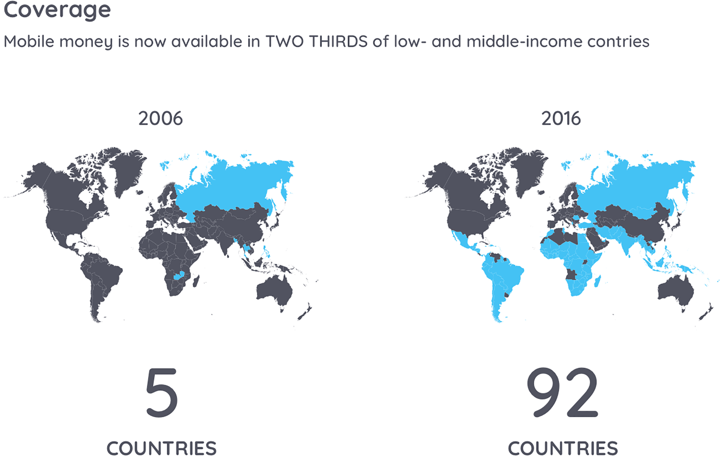
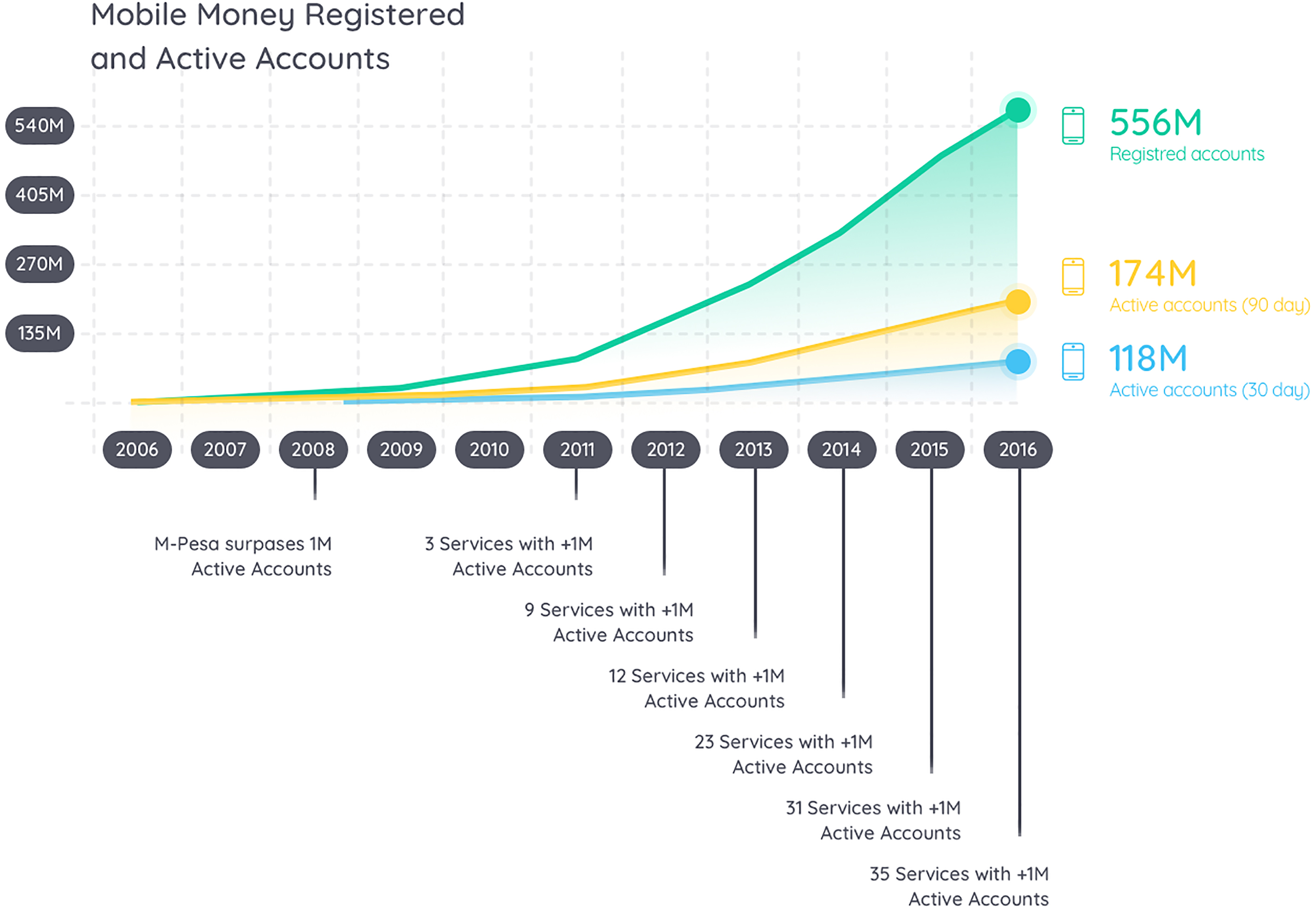
Some emerging market countries use mobile money. Mobile money refers to financial services operated in financial regulation and performed from or via a mobile device. This system, provided by a MNO, works like a bank account for the user. It allows several types of financial transactions, for example, bills payment and money transfer. These transactions generate the same type of data that a savings account in a traditional bank would generate. Since the use and coverage of mobile money is a growing trend, it has not been fully explored yet. As in 2005, only five countries supported this technology which has spread already to two-thirds of emerging markets as seen in Fig. 3. This figure shows only the availability of the service in a given country. However, not only more MNO are providing these services in different countries, but also the individuals in those countries are using the service more often for their different financial needs. In Fig. 4 we can observe an evolution from one million active accounts in 2008 to 174 million at the end of 2016. People in emerging markets are embracing this service to meet their financial needs.

Figure 4.
Evolution of mobile money accounts. Data from [17].

During the past year, MNO were processing around 30,000 transactions per minute [17]. The number of transactions per year grew from 1.2 billion transactions to 268 billion over the last decade. From these transactions, 68.7% are Peer-to-Peer (P2P) transactions and 12.5% are bill payment transactions. The vast proportion of P2P transactions is due to the way some small businesses operate. Instead of using cash or credit card, a person can buy fish to a local fish shop and pay by transferring from the mobile money account of the customer to the mobile money account associated with the fish shop. The bills payment transaction works the same as in developed and more mature markets. For example, a customer subscribes to a service, such as electric or telecommunication service. Bill payments can provide better insights about the acquisition level of the customers. Even if the P2P transactions can be used to acquire goods, it is not exclusive to such use. The data from this kind of transactions can be shared between the MNO and a financial services company.

Companies like M-Shwari [11] and InVenture, today known as Fifer Mandell et al. [13] have built services on top of mobile money to offer mobile savings and mobile credit. Mobile money data is a useful variable to discriminate among defaulters and non-defaulters. Nonetheless, the use of MNO data limits the ability of a business to grow since some of the emerging markets have a relatively low penetration of mobile money service [16]. On the other hand, companies like Stewart [28] and Harkness [15] focus more on the social media footprint. This approach is useful to evaluate customers with medium to high presence on the social media since is based on likes, friends and shares [12]. On the flip side, it struggles to discriminate when low or no information on social media is available, which can be the case in rural areas.

Other companies in the same sector claim to use machine learning on their evaluation pipeline. Based on their operational description, Kreditech [18], Branch.co [6] and Cignifi [10] state that the use of machine learning is core on their loan evaluation process.

Bravo et al. [7] presented how credit scoring can be helpful when lacking external data. Building a logistic regression using characteristics of micro-entrepreneurs. Bravo et al. [7] conclude that traditional variables, e.g. income, do not help to differentiate the risk of micro-entrepreneurs in a volatile market. A more similar case to ours is the MobiScore approach [21]. This approach is based on customers demographics and device logs as we intend to do. The main difference is that MobiScore studies the default for credit cards while we focus on short-term micro loans. The MobiScore proved that a scoring model trained with mobile network usage data can be useful to estimate the financial risk of a person. Macroeconomic variables can also be a factor to consider when lacking formal sources of financial data. The case presented in Blanco et al. [5] proposes the integration of macroeconomic variables and MNO features to build a reliable scoring model. The models include variables like rate of annual change of Gross Domestic Product (GDP) during loan term and rate of annual change in the cost of electricity during the loan term. These models performed better in terms of misclassification than the classic approach.

Regardless the main source of data (social/online, mobile or MNO), MFIs have been benefited from these new technologies, they now can create a branchless structure. With this new structure, MFIs solved two issues. First, MFIs have now better criteria to evaluate their customers. And second, the huge cost of brick and mortar scheme was eliminated [19].

After reviewing the cases of success shown above, we started experimenting with our data. First, we did the exploration of variables and exploration of the target to predict. As much of the details in this field remain unpublished due to business reasons, we could not rely on the plain variables as some of the cases relate since they do not show the total process of transformation.

We also needed a precise definition of the target variable, for business purposes, there is no difference between a customer that pays on time and a customer that pays five hours late. In the next section, we define and test the moment on which a customer will be labeled as “Overdue” and how the other features might affect this label.
3. Datasets, feature engineering, features selection and algorithm selection

Only a few works published about credit scoring present a detailed process of variable selection and transformation. Some of them present the features on a general view as we intend to. The MobiScore [21], refers to the use of personal information alongside the use of features extracted from the utilization of the services of the MNO. Blanco et al. [5], go further and propose the use of macroeconomic features mixed with customer data to estimate risk in a micro economic environment. For this study, we focus only on the features collected by the MFI.

We also analyze the effects of the definition of the target variable. In Van Gool et al. [30], a straight definition is set in base on installments. However, our case is based on loans paid in a one-time payment at the end of the period agreed between MFI and the customer to a maximum of 30 days. To define the target variable, we created two scenarios the first one defining the target variable as due date plus two days. And, in the second we defined the target variable as due date plus three days. We used these periods as in our market payment transactions can be delayed up to 72 hours to be effective in some cases. The delay is due to the banking infrastructure of the market.

3.1 Structure of datasets

This section describes the datasets used to understand the behavior of our customers. Several datasets are used for experimentation. Even though all datasets contain the same features, the transformation process, selection process and time horizon considered are different. In Fig. 5 we present the process of Extraction, Transformation and Loading (ETL) of data used to create the base for each dataset.

Figure 5.

Process of extraction and cleaning of datasets prior to transformations.

With this process flow, we created the first dataset, denominated ETL dataset. This dataset is used for the model selection that will be presented in Section 3.4.

The second dataset, from now on called dataset A, covers all the first loans granted to the customers. Only the completed loans were considered, meaning that only paid loans and loans which have passed their respective due date were used. The third dataset, called dataset B, consists of all loans granted and not only the first loan of each customer. As in dataset A, only completed loans were considered when generating this dataset.

Following the structure of dataset B we created two more datasets, dataset C, and dataset D. As seen in Fig. 6, dataset C and dataset D consider different time windows. Dataset C considers the application of the previous three months while dataset D expand this time horizon up to five months. Aforementioned will help us to test the hypothesis that models will require more fresh data to predict more accurately in this fast growing market. Notice that only dataset A considers only the first application of each customer. All others datasets contain all type of loans. This approach was initially used because the scoring models will only be used in the first request of each customer. However, the conditions of the loans are the same regardless the number of previously granted loans. This means that a new customer has the same interest rate, same maximum amount to request and same maximum length to request as a customer who had paid five loans already. Based on this, we decided to consider all applications in order to increase the sample size for datasets B, datasets C, and datasets D.

Figure 6.

Timeline of creation of datasets and the restrictions considered for each dataset.

All datasets combine demographics of customers, personal information, loan details, mobile network usage and mobile device features. We also included the performance of the loan (overdue or not) which is the target of prediction. In our scenario, a Non-Performing Loan (NPL) is a loan that has passed more than three days after due date and has not been totally repaid. Therefore this loan is considered as an overdue in the dataset and marked with 1 in the target variable.

The dataset A consists of 930 cases with 38.5% overdue loans and 61.5% paid on time loans. The datasets B, C and D contain 1,140 cases each with 43.5% overdue loans and 56.5% paid on time loans. The summarized variables on each dataset use a 30 days window, using the previous 30 days from the moment of the loan application.

3.2 Description of features

The variables can be grouped by source. First, we focus on personal information of the customer. This personal information, including demographics, is collected when the customer opens the mobile app for the first time. In this first interaction with our service, the user also needs to fill a profile. Some of the variables in the profile can be changed later on, e.g. employment status. This information can provide better insights about the acquisition level of the customers. Some variables refer to the goods the customers have (e.g., house, car) and details about their employment status (e.g., time employed, industry, role). It also collects information financial load of the customer as it collects the marital status and number of children. This type of data has been considered since the building of scorecards as in Schreiner [25] to the use of advanced classification techniques as shown in Van Gool et al. [30], San Pedro et al. [21], Blanco et al. [5], among others.

We also collected mobile phone network usage variables. These variables capture whenever the customer uses one of the services provided by the MNO, e.g. incoming or outgoing calls, SMS, Multimedia Messaging Service (MMS), etc. It has been proven that being a customer of a given MNO can have an impact when building a scoring model [3]. The hypothesis is that high tier customers will relate with high tier MNO. From the mobile phone, we also collect system information, e.g. mobile applications installed. With the categories of the applications installed in the device, we can create a complete profile of the customers. The applications installed work as the “likes” and “shares” presented in [12]. Providing an idea of the real interests of the customers.

Finally, we add loan characteristics and conditions: length, amount, and purpose of the loan.

Table 1
Table of features considered on datasets

Personal information

Age

Gender

Marital status

Education level

Number of children

Employment status

Ownership of house

Ownership of car

Monthly Income

MNO and device features

Airtime

Airtime top ups

Number of calls (Incoming, outgoing)

Number of SMS (Incoming, outgoing)

Device Manufacturer

Last mobile update

Mobile Applications installed

Loan characteristics

Loan amount

Loan length

Loan reason

Table 1 shows in detail the list of the features used. This list presents only the core variables, we did feature engineering to create the following variables:

•

debt_ratio $=$ amount requested/monthly income

•

telco_usage $=$ airtime/monthly income

•

income_split $=$ monthly income/number of dependants

•

average_top_up $=$ airtime/number of airtime top ups

•

delta_calls $=$ number of calls 0–30 days/number of calls 31–60 days

•

delta_sms $=$ number of SMS 0–30 days/number of SMS 31–60 days

The notation 0–30 days refers to the number of calls made in the last 30 days prior to applying for a loans, the same logic applies to 31–60 days which refers to the number of calls made from 31 to 60 days prior to applying. Note that for building the income_split we have used number of dependants which is calculated as 1 $+$ number of children as it considers that the applicant depends on itself. Some previous works also have a similar selection of variables. Such is the case of the MobiScore [21], which considers number of SMS and number of calls as relevant features. Also, Bjorkegren and Grissen [4] conclude that the use of mobile data usage patterns can be a valuable input to build a scoring model even when lacking formal financial history. Moreover, these variables were analyzed with independence tests in order to identify any relationship between variables. Chi-Square independence test was conducted for categorical variables which reduced as seen on 3. Variables like the level of education did not have enough impact on the target variable, therefore was not taken into account.

3.3 Exploration of variables

In this section we present the description of some variables alongside some of the analysis done previous to modelling. Note that due to business matters, we do not present absolute values, we present relative values of each variable.

Our first approach included a partial description of the population based on demographics. The population met some of the expectation from the business experts based in the emerging markets. The customers are mostly males between 26 to 35 years that are settled in the evaluated region since only 10.3% live at their current address for less than 2 years. The customers also present low level of dependants, since 53.46% are single and 56.98% do not have children.

The population reflected some of the realities of the emerging markets. One of these realities is that most of the customers own a car but do not own a house. Cars in emerging markets are priority over residence, mostly because people need to cover long distances to get the goods and services they need. Furthermore, 38.2% of the customers are self employed and they might use their vehicle for their respective business. However, in terms of employment customers do not seem very steady, we observe a high proportion of customers have less than one year at their current employment.

We found high levels of education in our population with 87.5% of the customers at university level. However, this does not seem to match regarding salaries, as we focus in microcredit and the microloan represents between 10%–30% of the monthly salary for 69.19% of the customers.

In our case, the missing values were replaced by zeros. This can be easily explained with the variable Date of Employment. The variable is only available to customers who have chosen “Employed” in the Employment status variable in the previous step, as is mandatory to fill all the fields before applying we know that the missing means that it does not apply to that customer. Afterwards, we transformed date-type variables into numeric variables, e.g. Date_of_Birth $\rightarrow$ Age. And finally, we filtered the dataset (by columns) in order to remove the variables that are useless for our purpose, e.g. Customer_ID. Find in Table 2 a more detailed descriptions of the numerical features.

Table 2
Descriptions of numerical variables

Feature	Mean	StdDev	Range
Age	32.9	6.4	[21-62]
Number of children	2.0	1.4	[0-6]
Monthly income (USD)	320.9	295.4	[55-840]
Airtime (USD)	13.5	18.7	[0-84]
Airtime top ups	4.2	1.8	[0-6]
Number of calls	105.5	62.7	[0-391]
Number of SMS	17.3	24.7	[0-325]
Mobile applications	67.2	54.7	[0-701]
Loan amount	60.0	22.3	[0-100]
Loan length (days)	26.9	6.1	[0-30]

After doing a general overview of the population we went into further exploration, we analyze relations between the categorical variables and the target variable. We applied discretization to age and debt_ratio (age_intervals and debt_ratio_intervals) in order to analyze any kind of existing relation.

For the evaluation of the categorical variables we used a balanced sample and evaluated the sample by Pearson Chi-square statistic and Cramer’s V. These test are based contingency tables an will help us identify if there is any relation between variables and the strength of that relationship. We did the tests considering alpha equal to 0.05.

Table 3

Result of evaluation of categorical features

Accepted features:

Age intervals

Own car

Number of children

Duration at current address

Employment status

Years of employment

Principal bank of customer

Marital status

Type of residence

State of the customers

Rejected features:

Debt ratio interval

Education level

Gender

Nonetheless, the relationship strength obtained by Crammer’s V is relatively low. We did not find significant relation between the debt ratio and the target variable due to the constrains in the amount requested by customers. The customers cannot request pass a certain amount of monetary unit and most of them request the maximum amount allowed. Since most of the customers request the same amount then the variable turns into a generic variable such as gender and education level. Notice that to these categorical variables we added other categorical variables. We show the analysis of the personal information only, same type of test were used for the MNO related features and the loans related features. With a defined set of variables, selected through statistical tests, we formed a dataset that was use for the exploration of the algorithms.

As in formal banking, we wanted to predict the likelihood that a customer will repay or not the loan requested. We had a mix of numerical and categorical variables as seen in the Section 3. However, we did not have a defined algorithm to deal with this problem. Over the last few years, different classification techniques have shown success in a diversity of scenarios related to credit scoring.

3.4 Algorithm selection

This section reviews the different implementations used to deal scenarios related to risk prediction. First, the MobiScore [21] shows that Decision Tree (DT), SVM and LR algorithms can create reliable scores when lacking of financial history. The main goal of the MobiScore is to reduce the default rate in credit cards for customers in emerging markets. For this task, MobiScore train classification algorithms mostly with mobile phone data gathered from the customers. The MobiScore concludes that mobile phone data can indicate the financial risk of an individual without the needing bureau information which is the core component in formal banking and developed economies.

In other case, Blanco et al. [5] show that Artificial Neural Networks (ANN) outperformed the traditional techniques for scoring. The ANN model was more accurate when predicting defaulters. The ANN was trained with both financial and non-financial from a Peruvian MFI. As in our case, the primary goal was to reduce the type II error which in this context is to classify a customer with bad credit as a customer with good credit, therefore granting financial products. The borrowers considered in Blanco et al. [5] are micro-entrepreneurs. Financial data from their micro-enterprise is used as input to train the scoring models.

Bjorkegren and Grissen [4] highlight how useful can mobile usage data be when used for credit scoring. For this case, the use of Random Forest (RF) proved to be accurate when differentiating between good customers and bad customers. The dataset used to train the RF contains borrowers from an emerging market in the Caribbean area. This dataset also lack traditional financial data used to train scoring models in developed countries.

Bayesian Networks (BN) have also been used for credit scoring and outperformed traditional techniques [3]. Although the implementation of the BN algorithm was used in formal banking in Turkey, the variables associated with the building of the bayesian net are not entirely financial. Variables that relate the customer with a given MNO were used to identify good borrowers, presenting once again that non-traditional data makes an impact while creating a reliable credit score.

With this evidence, there is not an algorithm that outperforms the others. Each scoring technique has been able to succeed when dealing with non-traditional data to predict financial risk in emerging markets. This is an indicator that the financial risk of an individual can be estimated using pure behavioral data when the financial data is weak or existent. Then, in order to select a model, we decided to train several algorithms with the same dataset and focus their performance in the test set.

To compare the performance of the models, we focused on two metrics: the Area under Receiver Operating Characteristic (AUROC) curve as a measure of the accuracy and the true positive rate, where overdue is the positive class. The true positive rate can be measure later on when applied to real cases as will be presented in the presentation of results. To compute the metrics we turned the outcome into a probability and compare to a threshold $T=$ 0.5. We used 10-fold cross validation to test the performance and grid-search for setting the hyper-parameters. For the SVM, the kernel had domain $\{\textit{`linear'},\textit{`rbf'}$ }, the parameter C had domain $\{0.1,0.2,\ldots,1.0\}$ and parameter gamma was from 10 ${}^{-6}$ to 10 ${}^{-1}$ . The algorithms were built using Weka Experimenter 3.8.0.

Table 4
Comparison of algorithms by AUROC curve and true positive rate

Algorithm	AUROC	True positive rate
Logistic Regression	90.41%	78.79%
SVM	85.06%	75.72%
Neural Network	89.29%	75.44%
Random Forest	80.65%	54.58%
Decision Table	79.13%	67.36%
Decision Tree	71.84%	65.53%
Naive Bayes	78.41%	63.09%
Bayes Net	76.33%	56.20%

As seen in Table 4, the top performers were LR, SVM and ANN. To build the ANN we tested from 1 hidden layer to N-hidden layers, being N the number of features in the input. However, the best performing ANN was built with 2 hidden layers. From these algorithms, we selected LR, SVM. This selection is the result of optimizing the cutoff of the algorithms, SVM prediction improved more than ANN with a sightly movement of the cutoff. In our case, we would prefer to have a model with better prediction of the bad customers even if this means to lose some prediction power in the good customers as the cost of default overweight the cost of opportunity.

4. Set of target variable

At first, we did not had a precise definition of the target variable. To define the target, we analyzed the behavior of the overdue loans. The main idea of this analysis was to determine what should be called an overdue loan in terms of how many days late after due date have passed without payment.

As presented in Fig. 7, most of the customers that do not pay on time, end up paying within the next three days after the due date. This effect is related to some of the payment methods available to the customers. Even if the customer pays on the day their loan is due, the payment transaction can take up to 48 hours to be registered. Therefore, seems like the customer did not pay in time.

Furthermore, concerning business, a customer with some hours or a day of late payment was not considered as a bad customer. In this order, the target variable for an application x was set as following:

$\displaystyle\textit{Target}(\textit{x})=\left\{\begin{array}[]{cl}1&\text{If % number of days in delay }>3\\ 0&\text{If number of days in delay }\leqslant 3\end{array}\right.$ (1)

With a precise definition of the target variable and a dataset structured as dataset A, we trained several models to select those with good performance.We used a second test in order to validate the hypothesis used on the target variable definition. This test compared the AUROC changing the target definition to:

$\displaystyle\textit{Target}(\textit{x})=\left\{\begin{array}[]{cc}1&\text{If % number of days in delay }>2\\ 0&\text{If number of days in delay }\leqslant 2\end{array}\right.$ (2)

Table 5

Comparison of algorithms for 3 days definition against 2 days definition

Algorithm	AUROC using 3 days	AUROC using 2 days
Logistic Regression	90.41%	84.97%
SVM	85.06%	74.60%
Neural Network	89.29%	81.50%
Random Forest	80.65%	79.31%
Decision Table	79.13%	76.70%
Decision Tree	71.84%	70.88%
Naive Bayes	78.41%	75.65%
Bayes Net	76.33%	74.31%

Figure 7.

Distribution of overdue by days late.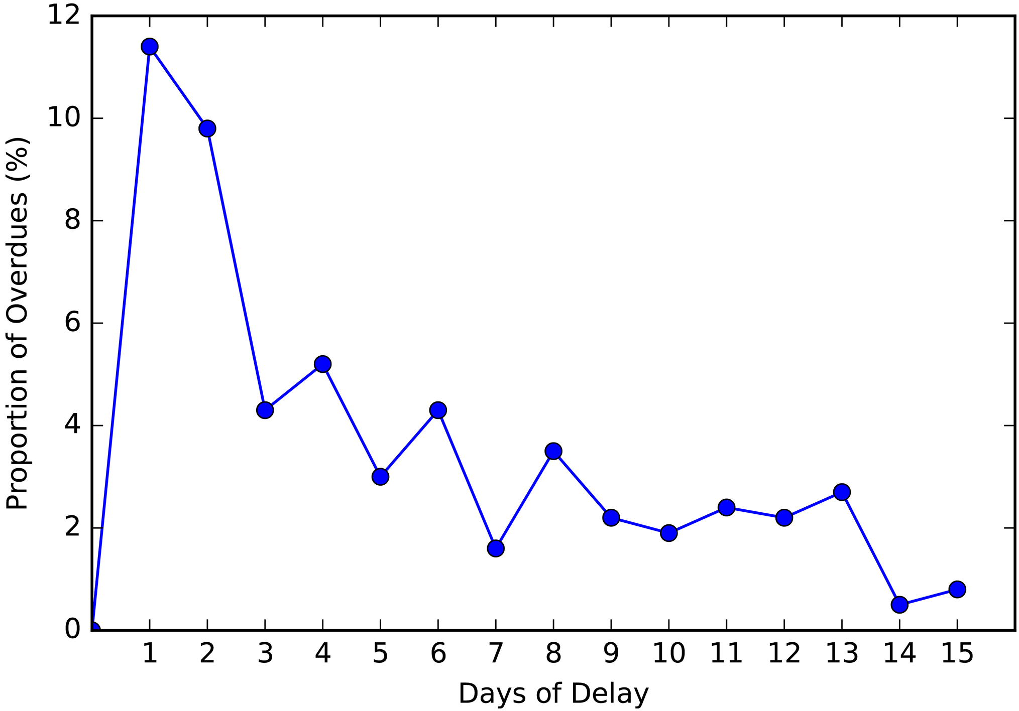

As presented in Table 5, the performance of each algorithm is worst when using the two days definition for the target variable. The performance also decays when we set the definition to one day. It is evident that the smaller the grace period conceded to be labeled as good borrower the harder to set statistical difference.

For each algorithm, we selected the one which settings provided the best performance. We used the grid-search to test each combination of parameters, changing the definition of the target variable as well. The algorithms selected in this phase, LR, and SVM, are the algorithms that we focus on for further experimentation. For feature selection we tried Recursive Feature Elimination (RFE), RF and WoE. The features presented in Table 1 are the variables that optimize the AUROC and the true positive rate, selected with the WoE. By comparing the AUROC and the true positive rate, we decided to use the target definition set in Eq. (1) for further experimentation.

5. Methodologies for the experiments

In this section, we present the structure of the different experiments undertaken. As presented in the Section 3, the target variable is a binary variable where 1 means overdue and 0 means paid on time. The classification task was modeled using supervised learning algorithms. Each entry will be processed to generate an output O which will be the estimated probability of going overdue.

We experimented using each dataset described in Section 3. The main differences between the first two experiments were the variable selection procedure and the transformation method used. We tested both transformation methods presented in Van Gool et al. [30], these are dummy variable transformation and WoE. Van Gool et al. [30] showed that both methods could be used to transform data to train a credit scoring algorithm. We tested both transformations methods in order to see which one suits better to our case.

San Pedro et al. [21] show how the different time windows can affect the performance of the credit scoring model. Following this reasoning, our third experiment focus on the time window considered for the training data. We compared the AUROC obtained after training the models with dataset C and dataset D.

5.1 First experiment: Implementing dummy variables

For the first experiment, we used dataset A. Our first step was to extend the dataset A by transforming the categorical variables into several (binary/dummy) variables. For variables with N categories we generated $N-1$ new variables, e.g. “Gender”:{‘Male’, ‘Female’} was turned into “Male”:{‘1’, ‘0’}. Date variables were transformed into time unit elapsed since the date referenced, e.g., date of birth turned into age.

In the second step, we applied an information gain ranker in order to select the variables that contribute to the classification task and drop those that create noise. We performed this selection using Weka Explorer 3.8.0, using both InfoGain and GainRatio as attribute evaluator with the Ranker method. The final step was to build the model itself, for this task we applied supervised learning algorithms to the transformed dataset to create the models.

Following the results presented in Table 4, the two primary classification methods that we focus on our experiments are LR and SVM. Not only LR and SVM performed better regarding AUROC but also these models make no assumption on the distribution of the input data, meaning they are quite tolerant to the input received [27]. We used 10-fold cross validation to test the performance of the algorithms using a given dataset. This validation technique helps us to maximize the use of the data as it uses each case both for training and validating. Through cross validation, we can also avoid overfitting issues. Our main metrics of evaluation were accuracy and approval rate. The recall is linked to the performance of the overdue class in the target variable. We choose these metrics so we can compare it with the baseline defined in the previous evaluation process. This comparison is key to know if we solved the main issue stated in Section 1. In our use case, we preferred to reduce the accuracy of the prediction of good borrowers in order to have better predictions in the overdue class; this approach is also presented in Blanco et al. [5]. For each algorithm, we used grid-search for setting the hyperparameters in order to optimize the evaluation measures. The output for each loan $O_{i}$ was then transformed into a probability $\textit{P}_{i}$ following the expression:

$\displaystyle{P}_{i}=\frac{e^{O_{i}}}{e^{O_{i}}+1}$ (3)

The models were applied to the new incoming loan applications on which the probability P for each new application was computed by the model and compared with a given threshold. The models evaluated only applications from customers who applied for the first time and customers with only one paid loan before.

5.2 Second experiment: Implementing weight of evidence

The second experiment was based on dataset B. In order to obtain comparable results, we tested LR and SVM algorithms again. For this dataset we used the WoE coding of variables. The WoE focuses on the odds ratio. Assume a variable $X$ with domain $\{X_{1},\ldots,X_{i}\}$ The WoE of $X_{i}$ is computed as:

$\displaystyle\textit{WoE}(X_{i})=\textit{ln}\left(\frac{\textit{TotalGoods}(X_% {i})}{\textit{TotalBads}(X_{i})}\right)$ (4)

In Eq. (4), TotalGoods( $X_{i}$ ) refers to the number of borrowers that paid on time for category $i$ in variable $X$ . The same concept applies to TotalBads( $X_{i}$ ) but considering the borrowers that went overdue. Note that the value of the WoE is 0 when both the distribution of the good class and the distribution of the bad class are equal. It indicates that the category evaluated does not allow to differentiate between classes. Using the recoded dataset, we calculated the Information Value (IV) of each variable. The IV for a category $i$ of a variable $X$ with $n$ number of categories is as follow:

$\displaystyle\textit{IV}(X_{i})=\frac{\textit{WoE}_{X_{i}}}{\sum_{i=1}^{% \textit{n}}\textit{WoE}_{X_{i}}}$ (5)

The IV for variable $X$ is the sum of the IV of each category $i$ of $X$ . It can be calculated as IV(X):

$\displaystyle\textit{IV(X)}=\sum_{i=1}^{i}\left[(\textit{TotalGoods}_{i}-% \textit{TotalBads}_{i})*\textit{ln}\left(\frac{\textit{Total Goods}(X_{i})}{% \textit{Total Bads}(X_{i})}\right)\right]$ (6)

After obtaining the IV for each variable, we follow the criteria presented in Siddiqi [26] to select the relevant variables. Siddiqi [26] proposes intervals to relate the IV to the strength of the relationship with the target variable. These intervals can relate the variable under analysis in order to determine a weak, medium, strong or non-existent relationship between the analyzed variable and the target variable. The relation can be set as shown in the conditions below.

When IV:

•

Less than 0.02, the variable does not differentiate the Goods/Bads odds ratio.

•

Between 0.02 to 0.1, the variable has only a weak relationship to the Goods/Bads odds ratio.

•

Between 0.1 to 0.3, the predictor has a medium strength relationship to the Goods/Bads odds ratio.

•

Equal 0.3 or higher, the predictor has a strong relationship to the Goods/Bads odds ratio.

Table 6

Example of IV calculation and WoE for variable X

Domain of X	Goods	Bads	Total	Dist. of Goods	Dist. of Bads	Cumulative IV	WoE
$X_{1}$	163	144	307	0.1451	0.1986	0.0168	$-$ 0.3137
$X_{2}$	78	15	93	0.0695	0.0207	0.0591	1.2111
$X_{3}$	316	123	439	0.2814	0.1697	0.0565	0.5060
$X_{4}$	23	12	35	0.0205	0.0166	0.0008	0.2130
$X_{5}$	198	152	350	0.1763	0.2097	0.0058	$-$ 0.1732
$X_{6}$	345	279	624	0.3072	0.3848	0.0175	$-$ 0.2253
Total	1123	725	1848	1.0000	1.0000	0.1565

In Table 6 we present an example of the calculation of IV and the corresponding WoE for each category of X. In the example, the values of each customer on the feature X will be replaced by the corresponding WoE for that category. A customer with $X_{1}$ on feature X will now have $-$ 0.3137 on feature X. The IV for variable X is 0.1565 meaning it has a medium strength relationship with the Goods/Bads odds ratio.

For the experiment, we selected the variables with weak, medium and strong relationship to the Goods/Bads odds ratio and trained the models. In Table 7 we present the IV of the selected features. In this experiment, we trained both algorithms using dataset B with the WoE transformation. As before, we used grid-search for setting the hyperparameters to optimize the evaluation measures and 10-fold cross validation to measure the performance. The output for each loan $O_{i}$ was transformed using Eq. (3) and then probability Pi of each application was compare to a given threshold. The models were applied to applications under the same criteria as the first experiment.

Table 7

Result of the WoE analysis

Feature	IV
Average top up	0.59
Employment date months	0.42
State	0.38
Delta calls	0.37
Number apps	0.36
Device manufacturer	0.36
Age	0.34
Total calls	0.31
Income Split	0.31
Loan Amount	0.27
Telco usage	0.22
Monthly income	0.22
Debt ratio	0.18
Delta SMS	0.16
Average airtime	0.13
Loan reason	0.10

5.3 Third experiment: Algorithm validity period

The purpose of this experiment is to have an idea of how long should a model be valid. We intend to analyze two events that we believe could affect the performance of a credit scoring model in the long run. As Blanco et al. [5] succeeded using macroeconomic variables in a microfinance problem. We decided to have a brief analysis and try to differentiate emerging markets from developed markets concerning financial indicators. Emerging markets present a more volatile economy. These constant movements into the economy can completely change the conditions of the target population in a shorter period than expected. We analyzed the yearly inflation in these markets, presented in Fig. 8. Inflation can be defined as the variation of the prices of goods and services over a period. It is evident that emerging markets suffer highers rates of inflation. This can easily translate into a lower acquisition level or payment capacity of an individual from an emerging market. Since, if the individual does not increase the corresponding income will be unable to keep up with financial obligations.

On the other hand, we have the constant growing of the number of customers with an average of 18.7% new users per month. This means that in less than 6 months we have double the amount of users. This has direct impact in the description of the population. The demographics, proportion of goods and bad borrowers, etc., all change in a fast pace. This growth is not limited only to the number of customers but also to different regions in the targeted country. These regions mix with the already existing customers creating a whole new description of the population.

Therefore, we decide to train credit scoring models using different time windows. Based on the erratic movement of the GDP and the contently high inflation rate, our hypothesis states that the models should perform better when trained with a relatively short time window. The use of different time windows can be a determining factor as seen in [21].

Figure 8.

Timeline comparing the yearly inflation rate of emerging markets against developed markets. Data from World Bank [32].

The third experiment is based on dataset C and dataset D. As seen in Fig. 6, we created both datasets at the same time. However, we considered different time windows. Using three months for dataset C and five months for dataset D. This means that if we generate both datasets today, an application made four months ago will not be considered for dataset C but will be considered for dataset D. We used transformed each dataset recoding with WoE. Afterwards, we selected the useful variables based in their respective IV. With the transformed variables we then trained a LR model and a SVM model for each dataset. For the training procedure, we used grid-search for setting the hyperparameters to optimize the evaluation measures and 10-fold cross validation to measure the performance as in previous experiments.

Concerning results and deployment, the first and second experiments were tested with real applications received after model building and deployment. As for the third experiment, the results will be obtained through cross validation, comparing the AUROC and overall accuracy.

6. Analysis of results

In this section, we analyze the result of the experiments described in the previous section. We group the results of the first and second experiment. As these experiments were applied to real cases, then we can compare the performance of the previous evaluation workflow. Also, the first and second experiment both focus on the transformation method of the training dataset. For the third experiment, we used WoE as it showed better performance on the previous experiments.

The result of the experiments was compared to a previous cohorts of loans. This cohort comprises the results of of 800 loans that were granted according expert rules. In order to review the performance of the models, we need to compare the overdue rate. This rate represents the proportion of NPL over the total loans granted which met the approval criteria of the models. Only loans that surpassed their respective due date were considered. The length of both experiments is 40 days, however, both experiments were running in different time periods. First, the LR trained with dataset A (LR-A) model and the SVM-A model were deployed and considered 484 and 366 real cases respectively. The second experiment kicked off five days after the end of the first experiment, with the deployment of the LR trained with dataset B (LR-B) model which considered 1,064 cases and the SVM trained with dataset B (SVM-B) model with 1,397 cases. At the end of the second experiment, we proceeded to evaluate the time windows for the third experiment. The third experiment, as presented in Section 5.3, is evaluated accuracy over an independent set which consists of 2,236 cases.

6.1 Differences between dummy variables and weight of evidence

In the first experiment, we implemented the two selected algorithms referred in Section 3.4 and used $A|B$ testing to select which model will evaluate the corresponding loan application. The number of the application was used to divide the population into two parts; this number is a sequence of natural numbers. Therefore, assigning the applications with odd application number to the LR algorithm and the remaining (even application number) to the SVM algorithm. Even though we used A|B testing, we still calculated and stored probability of default for each application using both algorithms. This means that if the loan application in evaluation met the threshold for both models, then the result will be counted for both models as well. But if the loan application met the threshold for either LR or SVM, then the result will only be stored for that particular algorithm.

Therefore, the overdue rate represented in the first and second experiment shows the performance of each application that met the approval criteria of the corresponding algorithm. The results presented in Table 8 compare the scoring models with the manual process. The manual process refers to the all applications received before the beginning of the first experiment. This process was based on expert criteria pipeline. From the manual process, we considered only applications from customers who applied for the first time and customers with only one paid loan before. We selected these applications to match the same population targeted by the models.

Table 8
Improvements of models in relation to the baseline

Model	Overdue rate	Approval rate
Experiment 1 LR	$-$ 26.45%	$-$ 4.33%
Experiment 1 SVM	442.19%	$-$ 91.91%
Experiment 2 LR	$-$ 115.50%	56.46%
Experiment 2 SVM	$-$ 196.80%	251.53%

Figure 9.

Comparison of overdue rate relative to baseline by days after deployment.

The two leading indicators to measure are the overdue rate and the approval rate. Our experiments were focused on these two indicators since they are the core of a stable and sustainable business model. A high overdue rate will make the business model unprofitable, while a low approval rate will not grant enough loans even to cover the operational costs.

First, we notice that both models of the first experiment failed to classify correctly the overdues, this translate into direct costs for the MFI. The LR from the first experiment improved the approval rate. However, the overall accuracy of the LR did not perform as expected.

Figure 10.

Comparison of approval rate relative to baseline by days after deployment.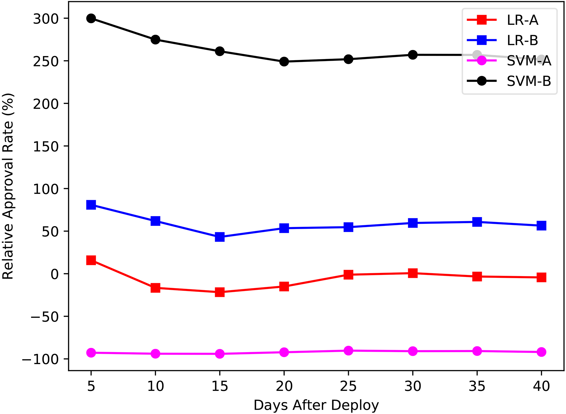

In Fig. 9 we compare the performance of the models in terms of classification error with real cases. The horizontal axis is the number of days after the deployment relative to the model under evaluation. Before the 30th day of deployment, both models trained with dataset A do not show overdue loans. This is due to the fact that the approval rate of LR-A and SVM-A was relatively low and just a few loans with less than 30 days of length were granted. However, after the loans granted by LR-A and SVM-A reached their respective due date, an increase on the overdue rate can be observed. Even if LR-A and SVM-A achieved a good overdue rate, these models would not be suitable for the business due to lack of approval. The models approved less than the baseline with $-$ 4.33% and $-$ 91.91% decrease of the approval rate respectively. Models trained with dataset B show a better behavior overall. Loans evaluated by LR-B and SVM-B presented fewer overdues and more evaluations were approved thought the evaluation by these models. As seen in Fig. 9, LR-B and SVM-B models are more stable on the overdue rate after the 30th day of deployment. These models are more constant and stable when compared to models created with dataset A. The LR-B and SVM-B models not only performed better in terms of overdue but also achieved higher approval rate than the manual process. As seen in Fig. 10, the SVM-B model was the best model in terms of approval rate. SVM-B was able to double the approval rate achieved by LR-B obtaining at the same time a slightly lower overdue rate. One of the main differences between the models, apart from datasets used for training, is the allocation of weights of the variables. Models trained with dataset A, gave more weights to variables related to the customer profile and loans conditions. The profile data of the customer is filled by himself and cannot be verified, thus making this data not really reliable. Furthermore, loans amount conditions are capped to a specific value, meaning they can only make variations within a small interval.

Figure 11.

Overdue rate relative to baseline by day of the week.

On the other hand, models trained with dataset B allocated more weights in variables related to historical data of the mobile phone of the customer. As the customer is not aware of its collection and/or cannot easily forged, these variables present a better profile of the customer and are more reliable, Both models trained with dataset B already surpassed the performance of the manual loan application selection process. More loans were granted when evaluated by the LR-B and SVM-B while the loans granted using the credit scoring evaluation presented fewer overdues.

While analyzing the performance of the models, we noticed some trends related to the nonpayment of the loans. As seen in Fig. 11, in general, the overdue rate for loans granted towards the end of the week is higher. This trend is also present in SVM-B which was the best model so far. LR-A also shows higher overdue rate in the last days of the week but concentrated on Friday and Saturday. LR-B shows less variation among the week days.

For Fig. 11 we did not consider SVM-A due to the low number of approved loans with this model. The low number is directly connected to the low approval rate.

Note that an overdue is not a total loss for the company since the overdue loans will enter into the recovery pipeline.

6.2 Results for different time windows

As for the third experiment, we compared the accuracy over a dataset composed of cases not present on the training set for any of the algorithms. For this we analyzed the status of the loan 30 days after due date and calculated the proportion of paid loans. In Table 9, we present the comparison of the accuracy by time window considered. With these results we cannot identify a clear winner as the difference is not significant.

Table 9
Third experiment: Comparison of accuracy after 30 days using different time windows

Model	3 months AUROC	5 months AUROC
Experiment 3 LR	90.87%	90.78%
Experiment 3 SVM	91.28%	91.37%

This result goes against the expectation when looking at the complete overview of the business. For the current trimester, the total number of customers increased by more than 50%. Moreover, the amount of granted loans for the same period of time resulted in more than 100% increase when compared to total granted loans prior to this period. However, we remain with the problem that the models get be quickly outdated. Based on the results of the third experiment we can conclude that the time window considered for training is not as relevant as the time window considered for updating the algorithms.

7. Conclusions and future work

As we have shown in the previous section, the use of credit scoring can be a useful tool to grant loans in emerging markets. Moreover, this problem seems to be one of the main upcoming challenges for MFIs in emerging markets. Every day, these markets have access to more technology that can help them in a way we have shown in this study. This is the start of a new era for MFIs which have overcome obstacle since first implementations by Yunus and the Grameen Bank.

One of this obstacles was the jump from group lending to individual lending. However, at beginnings of 2000, Mark Schreiner proved that credit scoring could be a useful tool for individual lending at a microfinance level, but it creates another issue, the collection of data was too complicated. The collection of data is already a history of the past since mobile devices allow to collect thousands of data points in an instant, these data points are useful as we showed in the exploratory analysis. The exploration of the data collected indicates that non-traditional features can be significant when identifying the financial risk of the customer. This data, combined with classification algorithms, can deal with the problem we presented at the start of this study which was to estimate the risk of the applicant in order to grant or deny the loan request.

Even though the first experiment did not perform as expected, both models trained with dataset B and the WoE recoding, proved to be better than baseline in both metrics used for evaluation. SVM-B and LR-B not only improved the overdue rate and the approval rate but also optimized the time of the loan approval pipeline. We believe that a two-month gap between training phase and deployment phase affected the result of the first experiment. As we presented in this study, the fluctuations of the market combined with the accelerated pace of business growth can out-date a model in a short period. For next steps we will be testing different time windows for updating the algorithms in order to keep the high performance that the models obtain in the first weeks of deployment.

References

Anderson

, The Credit Scoring Toolkit: Theory and Practice for Retail Credit Risk Management and Decision Automation, Oxford University Press, 2007.

Barnes

, E-commerce in emerging markets: The biggest growth opportunity, 2016.

Biçer

Sevis

and Bilgic

, Bayesian credit scoring model with integration of expert knowledge and customer data, In International Conference 24th Mini EURO Conference “Continuous Optimization and Information-Based Technologies in the Financial Sector” (MEC EurOPT 2010), Vilnius Gediminas Technical University Publishing House “Technika”, 2010, pp. 324–329.

Bjorkegren

and Grissen

, Behavior revealed in mobile phone usage predicts loan repayment, 2015.

Blanco

Pino-Mejías

Lara

and Rayo

, Credit scoring models for the microfinance industry using neural networks: Evidence from peru, Expert Systems with Applications 40(1) (2013), 356–364.

Branch.co, Branch, 2017.

Bravo

Maldonado

and Weber

, Granting and managing loans for micro-entrepreneurs: New developments and practical experiences, European Journal of Operational Research 227(2) (2013), 358–366.

Büthe

Yunus

and Jolis

, Banker to the poor: Micro-lending and the battle against world poverty, 2000.

Chen

Ribeiro

and Chen

, Financial credit risk assessment: a recent review, Artificial Intelligence Review 45(1) (2016), 1–23.

10.

Cignifi, Cignifi inc., 2017.

11.

Cook

and McKay

, How m-shwari works: The story so far, Consultative Group to Assist the Poor (CGAP) and Financial Sector Deepening (FSD), 2015.

12.

De Cnudde

Moeyersoms

Stankova

Tobback

Javaly

Martens

et al., Who cares about your facebook friends? credit scoring for microfinance. Technical report, University of Antwerp, 2015.

13.

Fifer Mandell

Strawther

and Zhu

, Inventure: Building credit scoring tools for the base of the pyramid, 2015.

14.

Fotabong

L.A.

, Comparing microfinance models, 2011.

15.

Harkness

, Big Data: Does Size Matter? Bloomsbury USA, 2016.

16.

Katakam

Frydrych

Murphy

and Naghavi

, State of the industry 2015: Mobile money, 2015.

17.

Katakam

Frydrych

Murphy

and Naghavi

, State of the industry on mobile money: Decade edition: 2006–2016, 2016.

18.

Kreditech. Kreditech – providing access to credit for the underbanked, 2017.

19.

Pickens

Porteous

and Rotman

, Scenarios for branchless banking in 2020. Washignton, DC: CGAP, 2009.

20.

Poushter

, Smartphone ownership and internet usage continues to climb in emerging economies, 2016.

21.

San Pedro

Proserpio

and Oliver

, Mobiscore: towards universal credit scoring from mobile phone data, In International Conference on User Modeling, Adaptation, and Personalization, Springer, 2015, pp. 195–207.

22.

Schreiner

, A scoring model of the risk of costly arrears at a microfinance lender in bolivia, Center for Social Development, Washington University in St. Louis., 1999.

23.

Schreiner

, Credit scoring for microfinance: Can it work? Journal of Microfinance/ESR Review 2(2) (2000), 105–118.

24.

Schreiner

, A scoring model of the risk of costly arrears for loans from affiliates of womenâ€™s world banking in colombia, Womenâ€™s World Banking, 2000.

25.

Schreiner

, The risk of exit by borrowers from a microlender in bolivia, Center for Social Development, Washington University in St. Louis, gwbweb.wustl.edu/users/schreiner, 2001.

26.

Siddiqi

, Credit risk scorecards: developing and implementing intelligent credit scoring, John Wiley & Sons, 2005.

27.

Sousa

Gama

and Brand ao

, A new dynamic modeling framework for credit risk assessment, Expert Systems with Applications 45 (2016), 341–351.

28.

Stewart

, Systems and methods for using online social footprint for affecting lending performance and credit scoring, 2014. US Patent 8694,401.

29.

Thomas

L.C.

Edelman

D.B.

and Crook

J.N.

, Credit Scoring and Its Applications, Siam, 2002.

30.

Van Gool

Verbeke

Sercu

and Baesens

, Credit scoring for microfinance: is it worth it? International Journal of Finance & Economics 17(2) (2012), 103–123.

31.

WorldBank, Financial inclusion: Helping countries meet the needs of the under-banked and under-served, 2013.

32.

WorldBank, World bank, 2017.

Credit scoring for microfinance using behavioral data in emerging markets

Abstract

Keywords

1. Introduction

1.1 Motivation

1.2 Problem definition

2. Related work

2.3 The arrival of big data

2.4 Non-traditional data In microfinance

3.1 Structure of datasets

Table 1 Table of features considered on datasets

Table 2 Descriptions of numerical variables

Table 4 Comparison of algorithms by AUROC curve and true positive rate

5.1 First experiment: Implementing dummy variables

6.1 Differences between dummy variables and weight of evidence

Table 8 Improvements of models in relation to the baseline

Table 9 Third experiment: Comparison of accuracy after 30 days using different time windows

References

Table 1
Table of features considered on datasets

Table 2
Descriptions of numerical variables

Table 4
Comparison of algorithms by AUROC curve and true positive rate

Table 8
Improvements of models in relation to the baseline

Table 9
Third experiment: Comparison of accuracy after 30 days using different time windows