
Abstract
This paper compares a number of state-of-the-art anomaly detection methods on real ship trajectories obtained by an Automatic Identification System (AIS) in the Baltic sea. Because most methods need fixed length trajectory representations, the paper also gives some solutions for reducing variable length trajectories to a fixed size.
Introduction
Maritime transport is the lifeblood of the global economy. It enables huge amounts of goods and people to be moved over long distances. However, maritime transport is also a source of significant threats, such as illicit weapon and drug trafficing, military operations, espionage, terrorism, piracy, illegal fishing, territorial violations, and pollution. Due to the fact that many of these threats are associated with behavior that drastically differs from normal, anomaly detection methods can be used to detect them.
There are two main classes of anomaly detection systems, that is, knowledge driven and data driven. Those that belong to the first class, usually, take the form of rule based systems in which the knowledge of experts is specified in the form of inference rules. The rules specify abnormal situations at sea, and each vessel behavior that matches at least one rule is considered to be anomalous. The more rules that are activated, the higher probability is that anomalous behavior has been identified. However, the problem is that the behavior of vessels does not always agree with the expectations of experts. It particularly applies to cases when the anomaly rules specify strict maritime regulations. Similar situations can be observed on our roads where car drivers often do not obey traffic regulations relating to speed limits.
Data driven systems focus on the measured typical behavior of vessels. Behavior that differs from the patterns of typical behavior is considered to be an anomaly. However, in order for the system to be able to effectively detect anomalies, a large amount of training data with examples of normal behavior needs to be acquired. The problem is that available data sets usually include examples of both normal and abnormal behaviors. It is very difficult to manually label (determine the class) all observed cases. To deal with this problem the data driven systems assume that normal cases dominate the abnormal ones in the training set. If it is not the case, the system will not be able to correctly detect anomalies.
Another categorization of maritime traffic anomaly detection systems refers to data that specify vessel behavior. In this case, two further types of systems can be distinguished, that is, point and trajectory systems. Point based systems make decisions based on momentary parameters of vessels such as velocity, position, course, etc. They simply focus on “appearance” of vessels at a single point in time. In contrast, trajectory systems analyze how the vessels behave over time, and make decisions based on a vector of vessel parameters collected over a period of time.
Because anomalies can take different forms which are often difficult to predict, and may change over time, effective anomaly detection systems should be modular and heterogeneous. Behavior of vessels at night may be different than during the day, the same applies to storm and nice weather, to a tanker and a fishing-boat, to open sea and mooring locations. Furthermore, different anomaly detection techniques have a specific way of operation, which can make them more, or less, appropriate to different forms of anomalies. Thus, it seems that a good practice is to split the systems into a number of sub-systems/modules, each responsible for different conditions at sea, type of vessel, sea area, etc. Furthermore, each sub-system should implement different anomaly detection algorithms with the goal of making the overall system sensitive to different forms of anomalies.
In order to make the system an effective tool for detecting anomalies, all of its components have to be appropriately prepared for the task. The effectiveness of each detection algorithm strongly depends on two factors, that is, data applied in the training/preparation process and the parameters of the algorithm. In the case of trajectories, the training data takes the form of varied length vectors whose components specify the state of a vessel at consecutive points in time. Since many detection algorithms operate on fixed sized vectors, the problem arises of how to reduce varied length trajectories to a common size. There are at least a number of methods which can be used for that purpose. However, in order to achieve high effectiveness in anomaly detection, the detection algorithm and the reduction method (that supplies the algorithm with input data) have to be adjusted to each other.
A further consideration is tuning the algorithm parameters, particularly the anomaly threshold, which is a central parameter since it regulates the sensitivity to anomalies and affects the false alarm rate. If the training set includes both normal and abnormal cases, and we do not know which cases are abnormal,1
Unsupervised anomaly detection [3] – usually, the only way is to manually label all the cases in the set which for big sets is very expensive and practically impossible, what is more, often, it is very difficult to evaluate whether the case is anomalous or it is not, note that wrong decisions while manual labelling may make the system insensitive to some dangerous anomalies.
The contribution of the paper is three-fold. First, it compares a number of state-of-the-art data driven anomaly detection methods on real AIS tanker trajectories from area of the Baltic sea near the Poland’s coast. Second, the tests with selected detection methods were performed in combination with different trajectory representation methods. Third, a simple solution that makes it possible to effectively tune algorithm parameters and evaluate its effectiveness was proposed in the paper and tested during reported experiments.
The rest of the paper is organized as follows: Section 2 provides overview of the field, Section 3 outlines trajectory anomaly detection methods used in the tests, Section 4 specifies trajectory reduction/representation methods applied in the tests, Section 5 reports the experiments, and the final section summarizes the paper.
A vast amount of literature exists on the topic of trajectory anomaly detection, also in the maritime domain. A comprehensive review relating not only to trajectories is given, for example, in [18]. The paper provides a high-level introduction to the domain, describes various steps necessary for anomaly detection, identifies gaps from different perspectives, outlines methods and algorithms, and provides their high-level assessment. The paper also presents a taxonomy of the methods from the field which, after some modifications, can be reduced to six general trajectory anomaly detection approaches: Rule Based (RB), Nearest Neighbor Based (NN), Classification Based (CL), Clustering Based (CLU), Auto-Encoder Based (AE), and Recurrent Neural Network Based (RNN).
Examples of the RB approach are presented, along with other things, in [13, 35]. In work [35], an ontology is used to represent the concept of semantic trajectories. Instead of operating on the low-level data from maritime sensors, the rule based expert system proposed in [35] operates on a high-level ontology. Abnormal ship behavior is detected by executing reasoning rules that refer directly to the ontology and which are defined by experts in the maritime domain.
Another interesting RB approach is Rule- and Motif-based Anomaly Detection in Moving Objects (ROAM) [13]. As in [35], the analysis of the trajectories is performed not at the level of low-level data, but at the level of movement patterns called motifs and their attributes. The trajectories are first decomposed into motifs, the motifs are specified with attributes, general or specific, and finally, a rule based system is run which analyzes attribute-value pairs to detect anomalies. The system, unlike the one proposed in [35], learns the rules automatically using an algorithm called Classification using Hierarchical Prediction Rules for that purpose.
The NN approach compares a new unlabeled case with all labeled cases stored in a database, the most similar labeled case (nearest neighbor) indicates the class of the new case. To classify the new case, the NN needs a similarity/dissimilarity measure. The Euclidean distance is perhaps the simplest and most natural dissimilarity measure. However, it requires trajectories to be properly aligned and of equal length [12]. To reduce varied length trajectories to one common size, methods can be used as described in [21], and in a further section of the current paper. In addition to the Euclidean distance, other measures which enable comparison between unequal length trajectories, are also used, for example, Dynamic Time Warping [20], Edit Distance on Real sequence [4], and Hausdorff distance [11, 12]. Such an approach is applied among other things in Similarity based Nearest Neighbour Conformal Anomaly Detector (SN-CAD) [11, 12, 32] which is based on Conformal prediction theory [37] and Hausdorff distance.
The disadvantage of the classical NN approach is that many calculations are needed in order to determine the category of the new case. To obtain the final result, all labeled trajectories have to be compared to the new one, for big data sets such an approach is impractical. An interesting alternative for ocean trajectories is presented in [30]. In this case, only one normal pattern trajectory is compared to the new one. The pattern trajectory is generated by means of the well known shortest path A-star algorithm, then, it is described by four different features, and finally compared with the input trajectory.
The CL approach has a number of representatives in point anomaly detection, that is, Neural Networks, Bayesian Networks, and one-class Support Vector Machines (SVM) [3]. In the trajectory domain, SVM was applied in combination with two different trajectory representations whose objective is to convert varied length trajectories into vectors of the same dimensionality. In [25], trajectories are sub-sampled, whereas in [22, 26], they are transformed into 2D and 3D discrete spatial representations. The idea of trajectory transformations proposed in [22, 26] was adopted in the research reported in the current paper. Apart from the representations detailed in [22], the paper proposes new solutions that along with the original ones were extensively tested and compared on real AIS data.
In addition to SVM, the Bayesian approach is popular in the CL [9, 19, 24, 38]. In [9], in addition to deviations from standard routes, the authors focus on other anomalous ship behaviors, that is, unexpected AIS activities, unexpected port arrival, close approach events, and zone entry events. The Bayesian network is then used to to carry out the anomaly fusion for threat assessment. With regard to trajectories themselves, the standard routes are defined between ports, oil rigs and other nodes specified in the environment, and all trajectories which deviate from them are considered to be anomalies.
In [19], the authors propose Bayesian networks for both point and trajectory anomaly detection. In the former case, the networks work on row AIS data, whereas in the latter one, the reasoning is performed on a track summary model supplied with different track characteristics, for example, the number of vessel stops, and stop locations.
The work [24] proposes the method called Traffic Route Extraction and Anomaly Detection (TREAD) in which trajectories are represented by route objects that consist of way-point objects such as stationary points, entry points, and exit points. The method incrementally generates, through DBSCAN clustering (see further), route patterns based on historical motion data, assigns the vessel track to a route cluster, and predicts the vessel trajectory based on the assigned route. If the prediction differs from the actual behavior by a threshold, an alarm is raised.
Dual Hierarchical Dirichlet Processes (Dual-HDP) is the method proposed in [38]. Even though its original application lies in language processing, the authors of [38] showed that Dual-HDP can be easily adapted to trajectory processing. Originally, the task of Dual-HDP is to cluster both words co-occurring in documents and documents themselves. In the trajectory domain, the task of the method is the same, however, documents become trajectories whereas words become the observations (positions and moving directions of objects) on the trajectories. In this case, abnormal trajectories are simply detected as cases with a low likelihood.
It seems that the CLU approach is the most popular among all anomaly detection algorithms. Example applications of the CLU approach in the maritime domain can be found in [1, 10, 14, 15, 16]. Roughly speaking, the general idea of the CLU is to group all available training data into a number of clusters, dense clusters represent normality, whereas sparse ones, abnormality. In order to classify a new case, membership degree to all clusters is calculated. Usually, three different options are then considered, that is, membership to a normal cluster, membership to abnormal cluster, or no membership to any cluster. The first case means normality, whereas the remaining ones abnormality.
In the AE approach [2, 28, 31, 33, 39, 36, 40], anomaly detection is performed by a feed-forward artificial neural network called an auto-encoder. In all the mentioned works, the general idea of network application is roughly the same. Typically, trajectories are converted into a fixed length representation, the network is trained with the use of only normal cases, and then, after training, the task of the network is to reconstruct an input trajectory representation on the network output. The reconstruction error decides about the normality or the abnormality of the trajectory.
The RNN approach [23, 34, 41] is the last anomaly detection approach that is considered in this paper. In this case, the task is to predict a next trajectory point knowing the previous points, the prediction error is accumulated over an assumed period, and if it exceeds a threshold, a trajectory is considered to be an anomaly. To this end, classical recurrent networks can be used and also those with Long Short Term Memory (LSTM) units [7, 17, 29].
Compared methods
In the experiments reported in the later sections of the paper, the following trajectory anomaly detection methods were compared:
The idea of DBSCAN is to group together densely packed points, that is, the points with many nearby neighbors. The points whose nearest neighbors are far away are considered to be outliers. Operation of DBSCAN can be expressed in the form of the algorithm specified in Fig. 1.
Pseudocode of DBSCAN.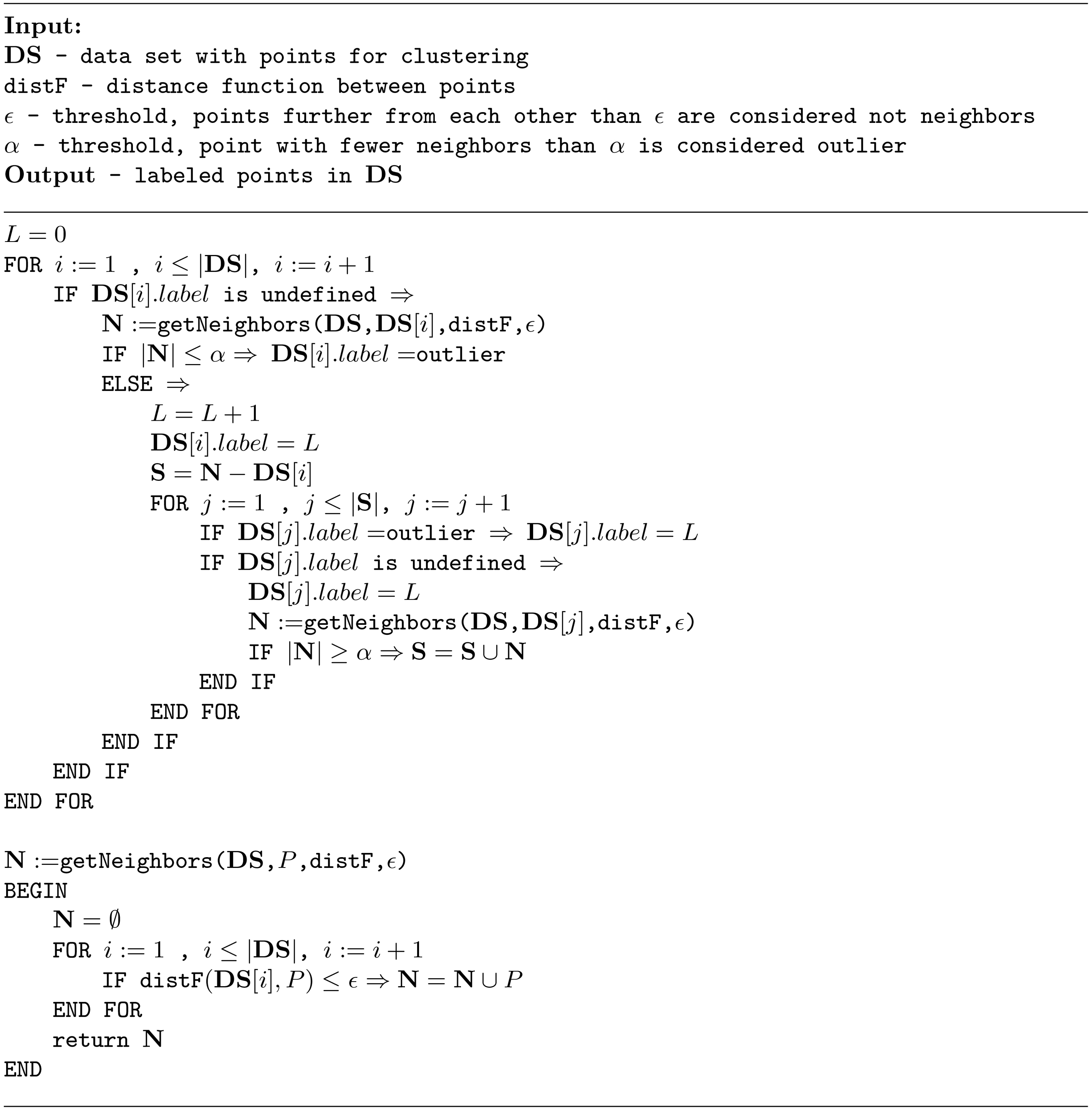
In GMM, K-means, and SOM, clusters are represented by centroids
In GMM, the centroids as well as covariance matrices
where
In the AE approach, as already mentioned, anomaly detection is performed by a feed-forward artificial neural network called an auto-encoder. A distinguishing feature of each auto-encoder is its layered architecture with encoder and decoder part and a code layer between the encoder and decoder. The number of encoder inputs is the same as the number of decoder outputs, and the number of encoder outputs is the same as decoder inputs and the number of nodes in the code layer. In shallow auto-encoders, the encoder and the decoder consist of only one layer, whereas in deep or stacked auto-encoders they include more than one layer. In the latter case, corresponding layers in the encoder and the decoder are usually of the same size. An example of a stacked auto-encoder is depicted in Fig. 2.
Schematic architecture of an auto-encoder [42].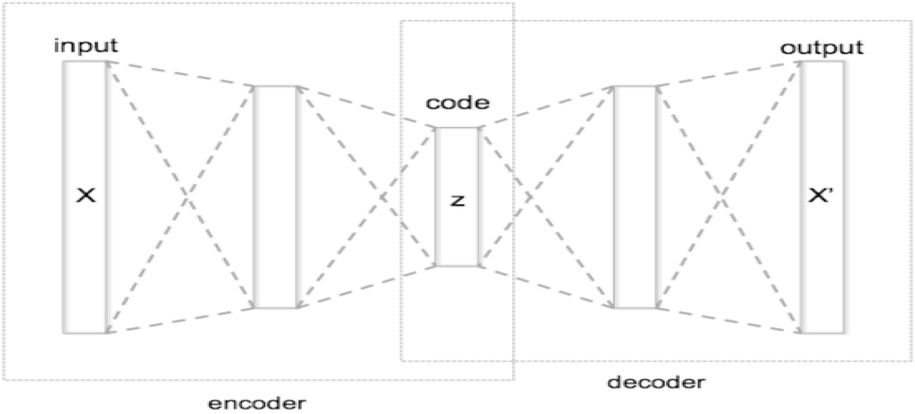
Usually, to train an AE, different variants of a well known back-propagation algorithm are applied. Although, other approaches like evolutionary algorithms or other global optimization techniques can also be used. Often, networks with many hidden layers need to be pretrained. A good practice is to train all hidden layers separately, layer by layer, and then to tune the whole pretrained network by means of the back-propagation algorithm. In the pretraining phase, Restricted Boltzmann Machines [6, 8] can also be applied which set the initial weights of neighboring layers through self-organization.
Auto-encoders applied to anomaly detection are trained to reconstruct the signal fed into network input. In this case, the assumption is that the training set contains mainly normal cases, the abnormal ones can also appear in the set but they are very rare. This way, the network is adjusted to normal cases and it learns to reconstruct them in the output layer. A properly prepared network should reconstruct normal cases with a smaller reconstruction error than the abnormal ones. The latter should be reconstructed poorly. However, the problem in this case is to find an appropriate threshold for reconstruction error.
The RNN approach, as its name implies, is based on recurrent neural networks. The networks are supplied with successive trajectory points, for example, longitude, latitude, COG, and SOG, and their task is to predict the subsequent trajectory point. The prediction error is accumulated over an assumed period, and if it exceeds a threshold, the trajectory is considered to be an anomaly. To this end, both classical networks and those with Long Short Term Memory (LSTM) units can be applied. The latter networks have proven their high effectiveness in many time series forecasting problems and for that reason they are becoming more and more popular among both researchers and practitioners. To train the networks, different variants of gradient decent algorithms are typically used. Evolutionary algorithms are an alternative technique which is also applied in the training process.
The difference between the RNN and other trajectory anomaly detection approaches is that the former works on original unprocessed trajectories which can be of varied length, trajectory points are analyzed one after another and an alarm is raised once the accumulated prediction error exceeds the threshold. Meanwhile, the other methods, typically, need trajectories reduced to a fixed size, and the detection process compares a trajectory representation with representations memorized in a database or encoded, for example, in the form of a neural network.
As mentioned earlier, many trajectory anomaly detection methods operate on trajectories reduced to the same fixed size. There are a number of methods which can be used for that purpose, and examples are presented in [21, 22, 26]. Some methods like Least Squares Polynomials, Chebyshev Polynomials, or the Discrete Fourier Transform [21] assume that trajectories are of higher dimensionality than their representations which make them useless if the above assumption is not met. Spatial representations presented in [22] do not impose any requirements on trajectory lengths, they measure the presence of a trajectory in selected points, say diagnostic points, of the trajectory point space. The number of the diagnostic points determines the dimensionality of the trajectory representation, the more points that are selected, the more accurate the representation and the higher its dimensionality is. In 2D trajectory point space, usually, it is enough to regularly distribute the diagnostic points on a 2D grid, whereas trajectory point spaces of higher dimensionality require other methods for point location, a good practice is simply to concentrate the diagnostic points in the areas of probable occurrence of the trajectories.
In the experiments reported in in Section 5, four trajectory representation (TR) and six diagnostic point distribution methods (DPD) were tested. For the purpose of this paper, the TR methods were called: SIMP, DIST, GAUSS, and PROB, whereas the DPD ones: REGULAR, RAND, REGULAR(N), and additionally GMM, K-means, and SOM.
REGULAR is only used in 2D space, and as the name implies, it regularly distributes diagnostic points on a 2D grid. RAND is a random method with a uniform distribution, whereas REGULAR(N) is a counterpart of REGULAR for
For each random population, an average distance between each pair of the points is calculated, the best population is the one whose the distance is the closest to
The SIMP method generates binary representations, where the
In the DIST representation, the
The GAUSS representation determines the degree of membership of each diagnostic point to the trajectory, the membership degree is Gaussian. Formally it can be defined as follows:
In turn, the PROB estimates probability of the
In the experiments reported in the further part of this paper, the following anomaly detection (AD) methods were compared: four CLU (DBSCAN, GMM, K-means, SOM), two RNN (classical recurrent networks and the ones with LSTM neurons), and AE. They were tested in combination with four TR methods: SIMP, DIST, GAUSS, PROB, and six DPD methods: REGULAR, RAND, REGULAR(N), GMM, K-means, and SOM.
Since all the experiments were carried out in 2D and 4D point spaces (see further), the decision was made to use the Euclidean distance in all TRs – dist in (4)
Real trajectories used in the experiments.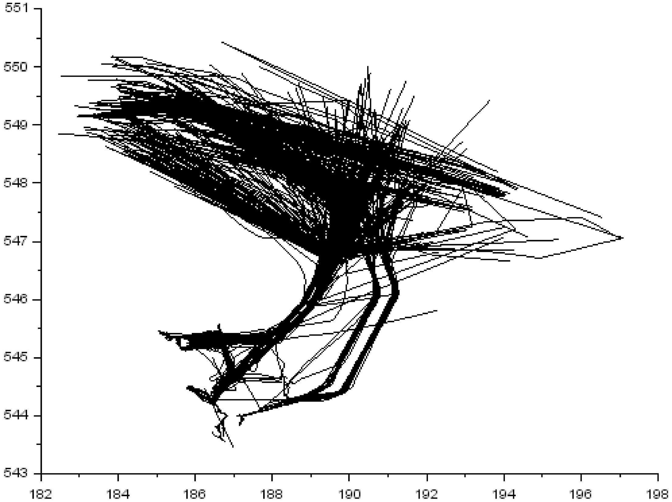
The comparisons were made on 534 unlabeled AIS tanker trajectories registered on the Bay of Gdansk (the Baltic Sea), all the trajectories are depicted in Fig. 3. 2D and 4D trajectories were applied, in the former case each trajectory point was described by latitude and longitude, whereas in the latter one SOG (Speed Over Ground) and COG (Course Over Ground) were also considered. For all the trajectories, the value of SOG exceeded 0.5 knots, the assumption was that anomaly detection applies only to vessels in motion.
Example random trajectories.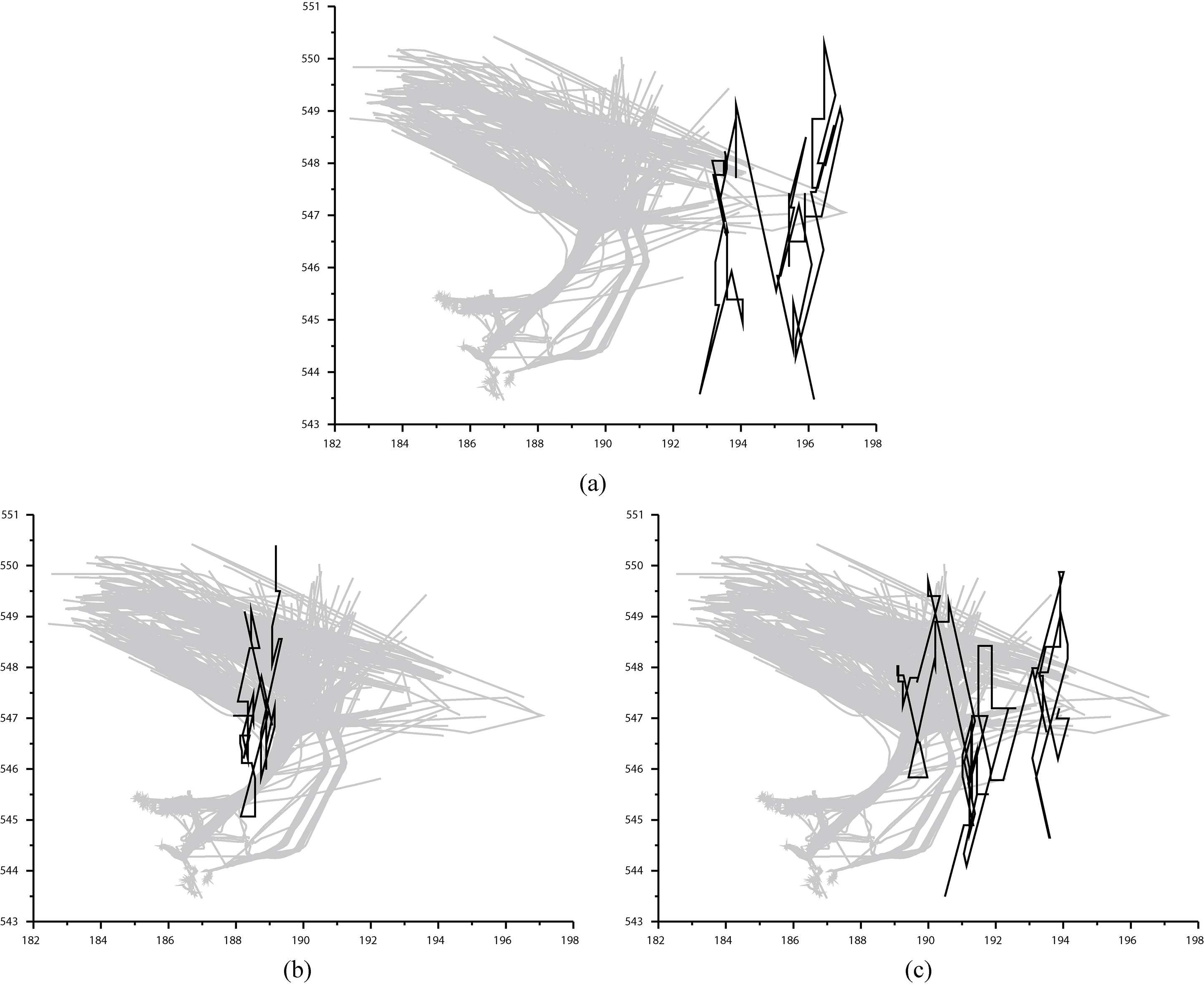
Since all the trajectories were unlabeled, the problem arose of how to tune each method to the problem, or in other words, where to place the dividing line between normal and abnormal cases. To overcome this problem, 60 extra 2D and 4D random trajectories were generated and used in the experiments as abnormal cases, example 2D trajectories are depicted in Fig. 4. 4D random trajectories were produced by adding SOG
Since the random trajectories significantly differed from the real ones, they could be considered as pure abnormal trajectories which should be all detected as anomalies. In other words, the anomaly detection methods could not make false negatives, false positives were the only acceptable errors whose number was used as an evaluation of the efficacy of each method. In spite of the fact that that the real trajectories, in addition to normal cases, could also include the abnormal ones, which should be detected, and whose detection should not be treated as error, the assumption was that each effective anomaly detection method should be able to correctly separate the two strongly distinct classes of trajectories. Thus, each detection among the real trajectories was in the experiments treated as false positive which had a negative impact on the evaluation of the detection method.
Generally, in the case of anomaly detection problems in which only unlabeled cases are available, applying random trajectories seems to be a good method for the estimation of a threshold that decides what is an anomaly and what is not. Everything that is close to that threshold should be carefully examined as a potential abnormality.
All the experiments were carried out in four phases. First, the diagnostic points were generated which were necessary for the construction of the trajectory representations. The second phase was devoted to the trajectory representations, which in turn, were necessary for training AD methods and final comparison tests. Since, after the second phase, a lot of different representations were produced, it was necessary to select a set of representations for further processing, and that was the purpose of the third phase of the experiments. Finally, all the AD methods were trained and tested on representations selected before.
The diagnostic points were generated, for
The second phase was devoted to trajectory representations. For each set of diagnostic points, 8 representations were generated, one representation for SIMP, one for DIST, three for GAUSS, and three for PROB. Individual representations of GAUSS and PROB differed in
The task of the third phase was to determine the most effective representation for each combination of
Results of the third phase of experiments for
Example diagnostic points for 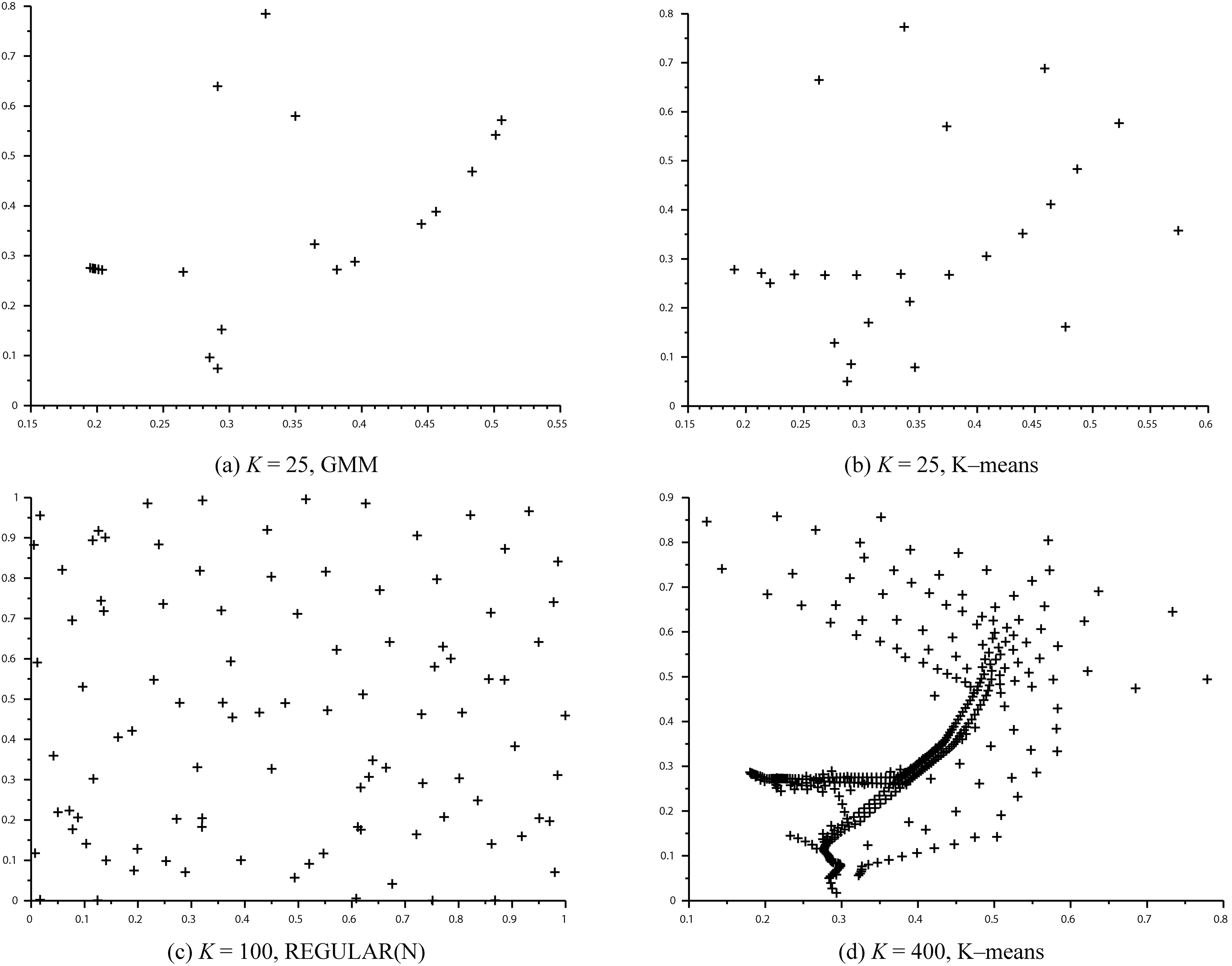
Example representations of a trajectory depicted in subfigure (a) for 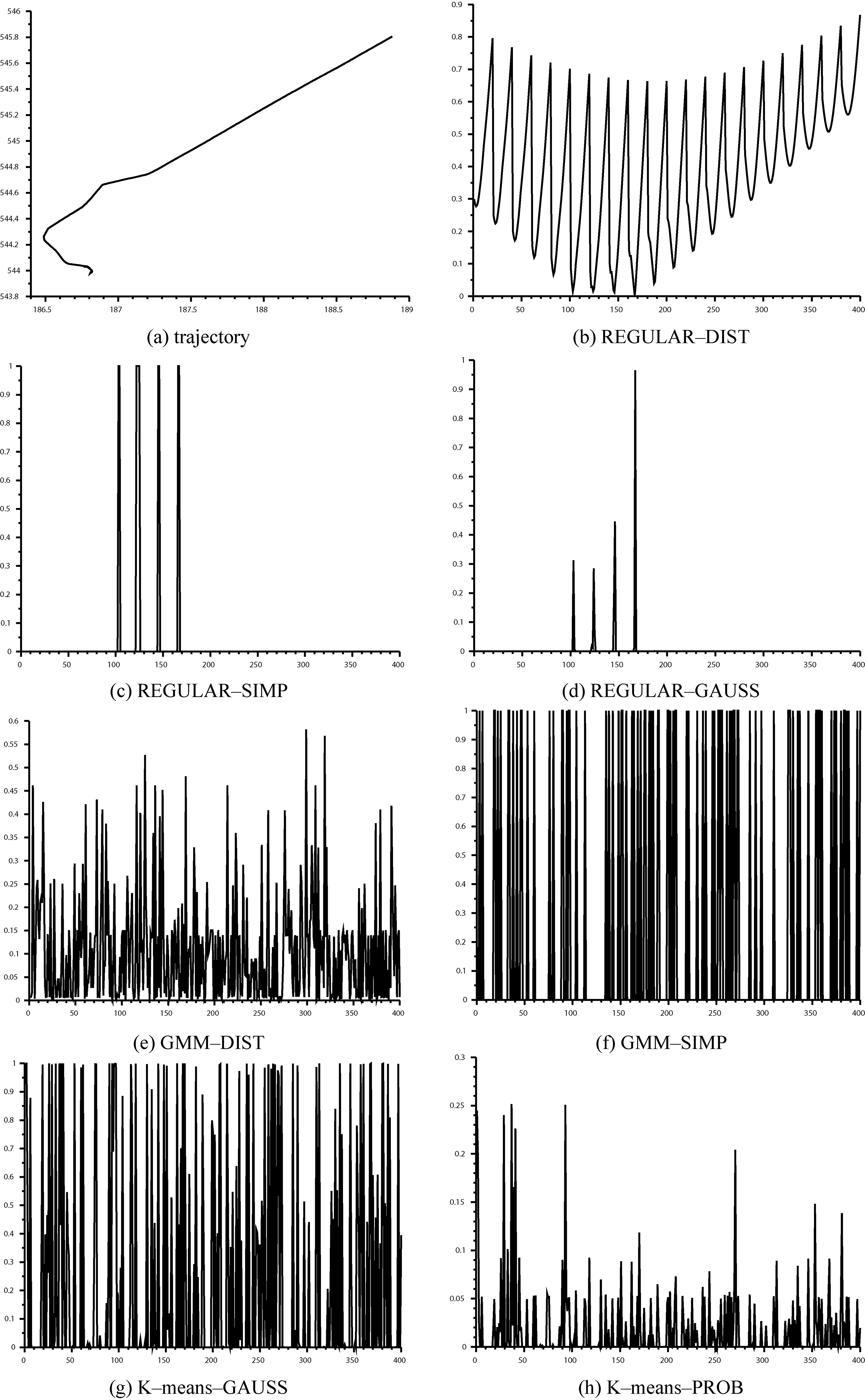
Results of the third phase of experiments for
Results of the third phase of experiments for
They show that for
As expected, for
Results of the third phase of experiments for
Results of the third phase of experiments for
For
With regard to trajectory representation methods, the most profitable solution for
Results of the comparison tests for
After the third phase of the experiments the following representations were considered to be optimal: REGULAR-GAUSS (
Before performing such a comparison, each anomaly detection system was trained on selected representations of the real trajectories, the random ones were not used in this process. To train CLU systems, appropriate clustering algorithms were applied, each algorithm was run many times for different parameter settings.
Results of the comparison tests for
Training auto-encoders took place with the use of a well known back-propagation algorithm. In this case, the plan was to gradually increase complexity of network architectures, initially, shallow architectures with only one hidden layer (25–10–25, 100–40–100, and 400–100–400) were to be examined, then, deeper networks were planned for final usage. However, the first tests showed that the deeper architectures are unnecessary, and shallow auto-encoders were sufficient to satisfactorily solve the problem.
To prepare RNNs, both classical and ones with LSTM units, an evolutionary technique called Assembler Encoding with Evolvable Operations (AEEO) [27] was used. As before, network architectures were supposed to grow gradually, for
Results of all the comparison tests are summarized in Tables 6 and 7. They show that the only method that was able to perfectly separate the real and random trajectories for all analyzed cases is the AE. It is worth noting that, as mentioned above, shallow AE architectures with only one hidden layer were sufficient to perform the task. Example errors of the AE while reconstructing all the trajectories applied in the tests are presented in Fig. 7. The figure shows that AE detectors had practically no problem to distinguish the real and random trajectories, reconstruction errors of the latter were considerably higher than the former.
Example reconstruction errors of the AE, numbers of real trajectories are from 1 to 534, the remaining trajectories are random.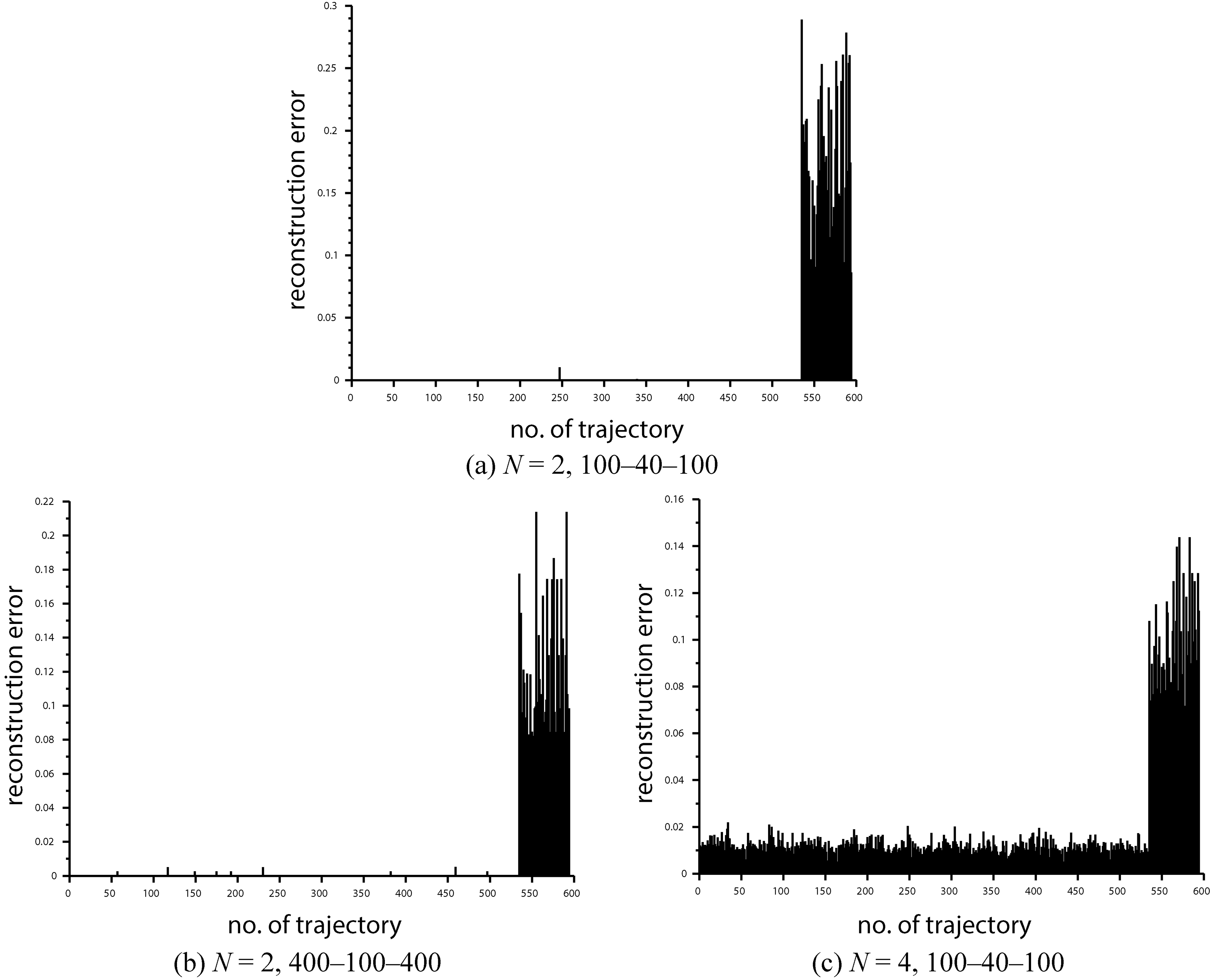
The CLU approach appeared generally to be slightly less effective. For
Example probabilities of abnormality calculated by GMM detectors.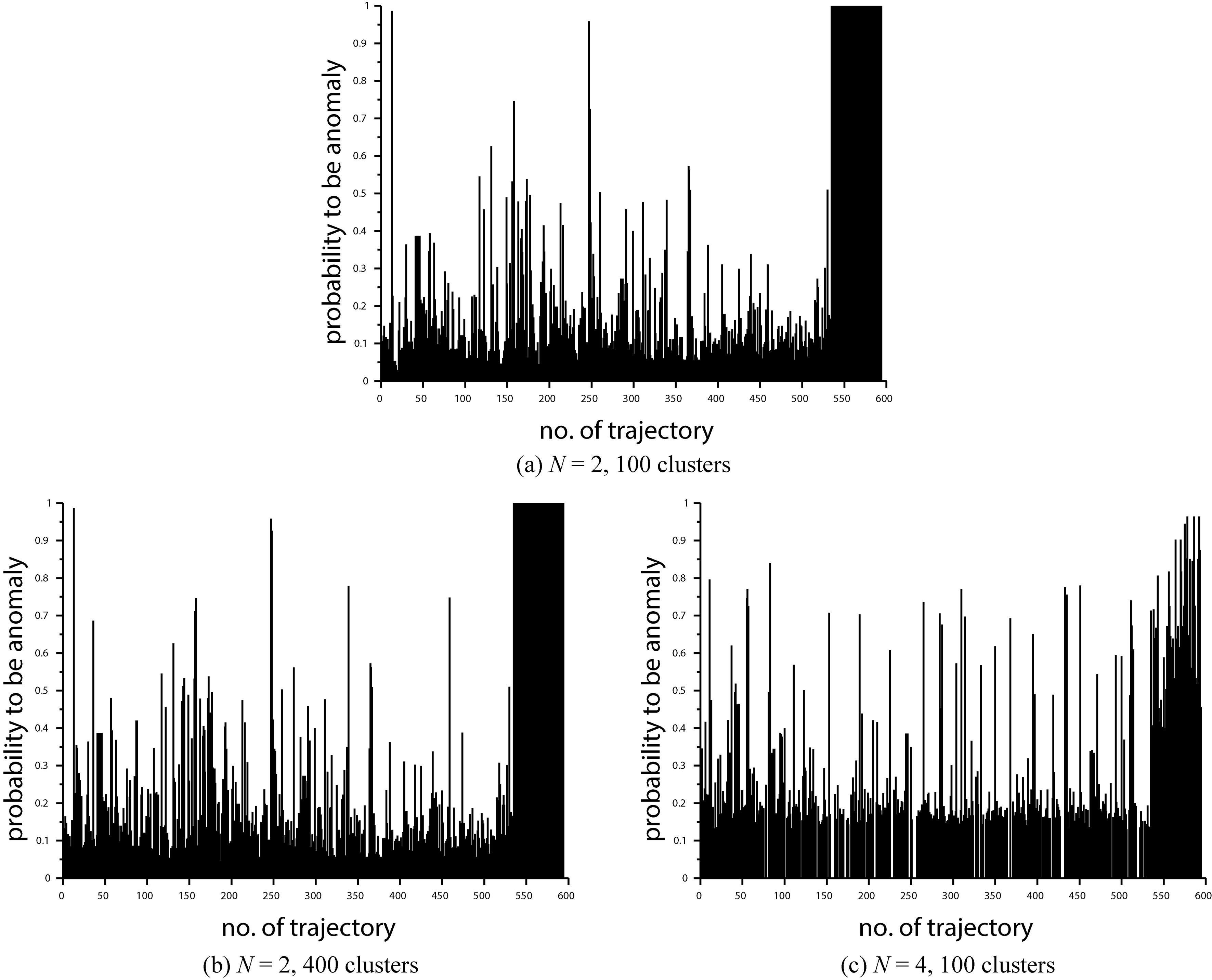
Unfortunately, for
One may suggest that the worse result of the CLU algorithms for
The RNN detectors achieved the same result for
Real trajectories classified by RNN as anomalies.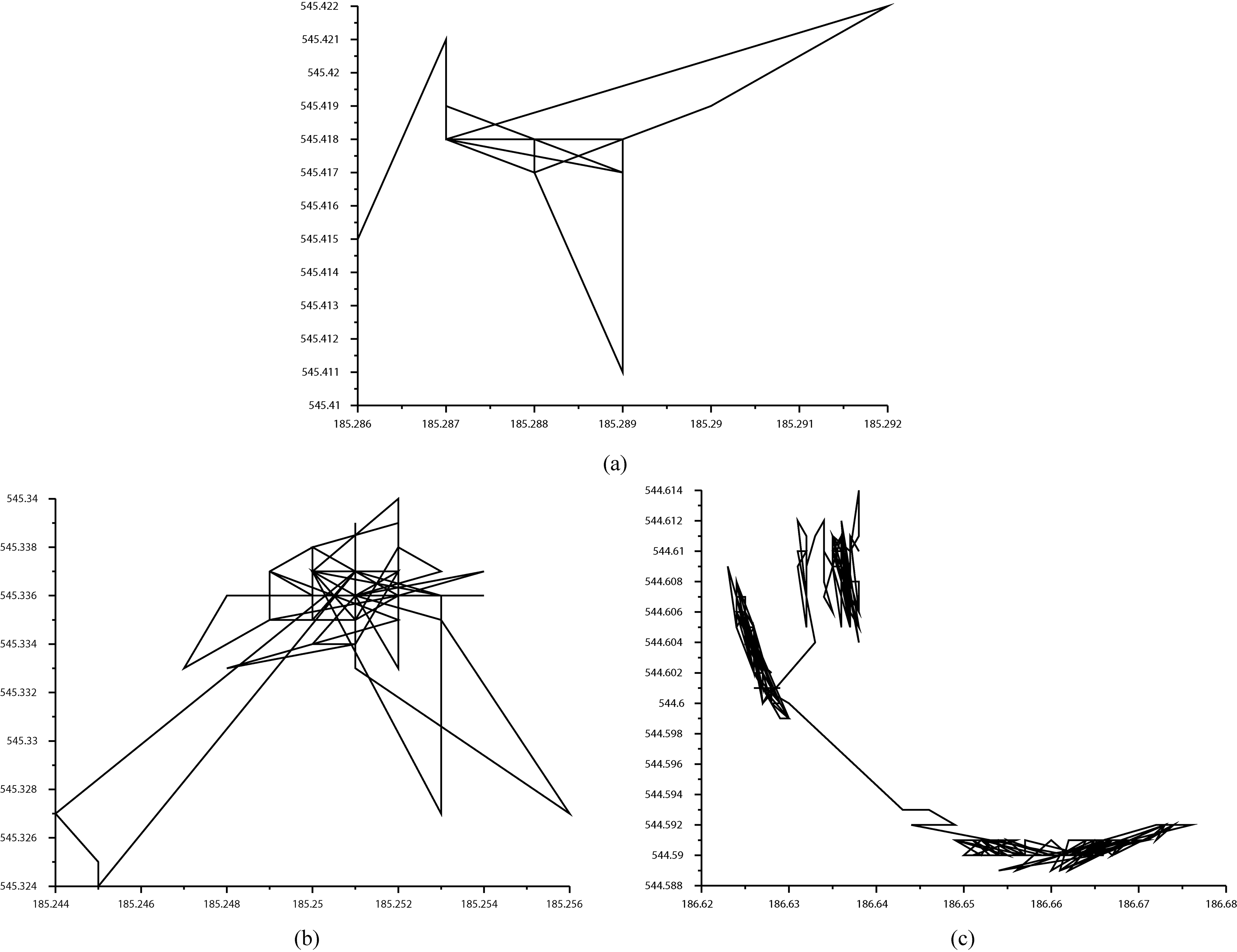
Real trajectories with the highest degree of abnormality indicated by AE (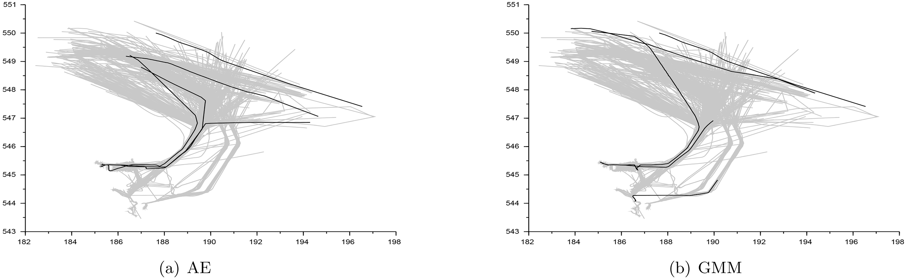
Of course, the random trajectories can be also considered chaotic, in this case, however, the chaotic movements are in a large scale. At the level of consecutive way-points, the random trajectories are linear, and in consequence, they are easily predictable. In the chaotic trajectories, movements between successive way-points are each time in a different direction, whereas in the random ones, the moves are exactly in the same direction for a long time, the change of direction is very rare compared to the number of way-points in trajectory. This way, the chaotic trajectories were often more abnormal for the RNN detectors than the random ones which, in turn, contributed to serious problems with their correct classification.
Since the remaining detectors work on spatial representations of trajectories, they were insensitive to the chaotic trajectories. The latter were almost point trajectories with very simple representations that were very easy to learn and memorize as normal. In this case, a rare presence in trajectory point space and/or a rare trajectory direction decided between normality and abnormality. Example real trajectories considered by the AE and GMM as normal, however, with the highest degree of abnormality among the real trajectories are presented in Fig. 10.
The paper compares a number of state-of-the-art anomaly detection methods on real marine trajectories. Comparisons were made for different trajectory representations, and for different trajectory dimensionality. The experiments reported in the paper revealed that for 2D trajectories the most suited representation is SIMP which is nothing but a binary barcode of each trajectory. Moreover, it appeared that regular organization of diagnostic points is, in this case, the most beneficial.
For 4D trajectories, representations which gather information from larger areas of trajectory point space turned out to be more effective than SIMP. What is more, due to enlarged diagnostic space, the regular distribution of points was not the only useful solution, distribution methods that randomly locate the diagnostic points and do it in concentrations of trajectory points were equally effective.
With regard to the anomaly detection methods, the experiments revealed that solutions based on auto-encoders outperforms all the others. Both in the 2D and the 4D case, the AE detectors were able to faultlessly classify all the trajectories. The CLU methods dealt with the problem well but only in 2D case, for 4D trajectories, they were noticeably worse than the AE. In turn, the RNN, that is, the only solution applied in the comparison tests which operated on unprocessed trajectories, appeared to be very sensitive to chaotic trajectories being the result of GPS errors. This sensitivity did not allow the RNN to produce even a single detector able to correctly solve the problem.
A serious problem while preparing anomaly detection systems supplied with only unlabeled cases is often to properly determine the anomaly threshold which is the dividing line between normal and abnormal. In the experiments, this problem was solved thanks to the random trajectories that played the role of the abnormal cases. This solution made it possible to estimate the threshold and to indicate potential abnormalities among unlabeled trajectories.
If the paper was to be an indication for professionals dealing with the problem of ship trajectory anomaly detection, it seems that all the experiments reported in the paper suggest the following:
For 2D points spaces: use SIMP representation with regularly distributed diagnostic points, For spaces of higher dimensionality: use GAUSS or PROB representations combined with computationally simple RAND or REGULAR(N) DPD methods, Use AE for anomaly detection, Use random trajectories to determine the anomaly threshold.