DNN models based on dimensionality reduction for stock trading

Abstract

In order to avoid missing representative features, we should select a lot of features as far as possible when using machine learning algorithms in stock trading. Meanwhile, these high dimensional features can lead to redundancy of information and reduce the efficiency, and accuracy of learning algorithms. It is worth noting that dimensionality reduction operation (DRO) is one of the main means to deal with stock high-dimensional data. However, there are few studies on whether DRO can significantly improve the trading performance of deep neural network (DNN) algorithms. Therefore, this paper selects large-scale stock datasets in the American market and in the Chinese market as the research objects. For each stock, we firstly apply four most widely used DRO, namely principal component analysis (PCA), least absolute shrinkage and selection operator (LASSO), classification and regression trees (CART), and autoencoder (AE) to deal with original features respectively, and then use the new features as inputs of the most six popular DNN algorithms such as Multilayer Perceptron (MLP), Deep Belief Network (DBN), Stacked Auto-Encoders (SAE), Recurrent Neural Network (RNN), Long Short-Term Memory (LSTM), Gated Recurrent Unit (GRU) to generate trading signals. Finally, we apply the trading signals to conduct a lot of daily trading back-testing and non-parameter statistical testing. The experiments show that LASSO can significantly improve the performance of RNN, LSTM, and GRU. In addition, any DRO mentioned in this paper do not significantly improve trading performance and the speed of generating trading signals of the other DNN algorithms.

Keywords

Deep neural networks dimensionality reduction statistical test trading performance

1. Introduction

Stock investment is one of the most important economic activities. Generally, investors make stock trading decisions based on the prediction of future stock price trends. However, forecasting stock price trends is a great challenge for investors and researchers. In the past many years, researchers have mainly constructed a statistical model to describe the time series of stock price to forecast the trends of future stock prices [1, 2, 3, 4, 5, 6, 7, 8, 9]. It is worth noting that traditional machine learning (ML) methods [10, 11, 12, 13, 14, 15, 16, 17, 18, 19] such as support vector machine [11, 12, 13] and random forest [14, 15], have shown strong ability in the trend prediction of stock prices. These algorithms can effectively capture the dynamic changes in the financial market, discover trading signals of some stocks, and make automatic investment decisions. When using machine learning algorithms to predict the trends of stock price, which features to be used as the inputs of the learning algorithm is one of the most important problems that researchers need to consider. The processes are called feature engineering. Generally, researchers choose as many features as possible to describe the research topics according to their own understanding of the problem and their knowledge backgrounds. In fact, they do not know which features can improve the ability of machine learning algorithms, but to blindly increase the number of features. However, it is generally believed that too many features will lead to redundancy of input information and make the machine learning models too complex, thus reducing the generalization ability of the learning model and the robustness of out-of-sample prediction. Therefore, DRO is a very important part of feature engineering and largely affect the performance of ML algorithms.

In recent years, artificial intelligence computing methods represented by DNN models have made a series of major breakthroughs in the fields of natural language processing, image classification, and voice translation and so on. It is noteworthy that some DNN algorithms have applied in stock price time series prediction and quantitative trading [20, 21, 22, 23, 24, 25, 26, 27, 28, 29, 30, 31, 32, 33, 34, 35, 36, 37, 38, 39]. However, most of the previous studies mainly choose a few stocks according to the researcher’s own preference [15, 17, 18, 20, 23, 25, 29, 34], or use the traditional machine learning algorithms combined with some DRO [17, 40, 41, 42, 43, 44, 45, 46, 47, 48, 49, 50] to predict the future stock price trends based on a few stock datasets. Meanwhile, there is a lack of statistical significance test between the trading performance of the prediction algorithm based on different DRO [25, 28, 40, 42, 47]. Therefore, the performance of back-testing may tend to be more optimistic. As far as we know, there is no study on the comparative analysis between the trading performance of DNN models based on different DRO, so whether DRO can significantly improve the trading performance of DNN models is a question worth discussing. The problem constitutes the main motivation of this research. The solution of the problem is of great value for practitioners to recognize the effect of the DRO on DNN models in the stock trading.

In this paper, we select 424 S&P 500 index component stocks (SPICS) and 185 CSI 300 index component stocks (CSICS) as the research objects and the stock symbols are shown in Appendix 1. Then, we construct the 44 technical indicators for each stock in the two markets such as the relative strength index and Bollinger bands as features are shown in Appendix 2. The label on the T-th trading day is the sign of daily return rate of the $T+1$ -th trading day. That is, if the daily return rate is positive, the label value is set to 1; otherwise 0. For each stock, we choose the technical indicators of 2000 trading days before December 31, 2017 to build a stock dataset. After the dataset of a stock is built, we apply walk-forward analysis (WFA) method to train the DNN models. In each round of training, we firstly use four most widely used algorithms (PCA, LASSO, CART, and AE) to do the DRO. Then we train six most popular DNN structures (MLP, DBN, SAE, RNN, LSTM, and GRU) based on the data after DRO and use the trained DNN models to forecast the trends of stock price. Finally, we use non-parameter statistical testing methods, the performance measure indicators (winning ratio (WR), annualized return rate (ARR), annualized Sharpe ratio (ASR), and maximum drawdown (MDD)), and the execution speed indicator (average training time of generating the trading signals of an individual stock (ATT)) to evaluate the differences between the trading performance of trading algorithms mentioned in this paper.

The experimental results show that LASSO is an effective DRO and it can significantly improve the trading performance of RNN, GRU, and LSTM both in SPICS and CSICS. In addition, any DRO mentioned in this paper cannot significantly improve the trading performance of the remaining DNN algorithms. In particular, these DRO cannot significantly improve the ATT of any DNN algorithms and even some DRO make the speed of generating trading signals significantly slower. In a word, most of DRO methods used in this paper do not have a significant effect on the promotion of trading performance and the execution speed of the DNN algorithms. Therefore, we need to re-understand the significance and value of DRO, which is of guiding value for implementing DRO in DNN algorithms.

The remainder of this paper is organized as follows: Section 2 reviews statistical models, DRO algorithms, and the stock forecasting models based on DNN models in the existing literature. Section 3 gives the architecture of this paper. Section 4 describes the method of data acquisition, the reason for selecting stock datasets, and data processing tools. Section 5 describes the methods of data preparation, stock dataset generation, and DRO methods. Section 6 gives parameter settings of the DNN models, the algorithm for generating trading signals, and trading strategy. Section 7 gives the trading performance measure indicators for back-testing and uses a non-parameter statistical test to analyze and evaluate the performance of the DNN models based on different DRO in the two markets. Section 8 provides a comprehensive conclusion.

2. Literature review

Predicting the future price trends of stock is very difficult for investors, but many academic researchers and industry practitioners are trying to apply various theories and methods to complete this task. The methods of predicting the directions of stock movement also change from the early statistical models to DNN models. In this process, a large number of theoretical research results and trading rules that can be used for actual trading have also been produced. Next, we review the latest development of statistical models, DRO algorithms, and DNN models in stock trading.

2.1 Statistical models

Statistical models are considered the state of the art for time series modeling and prediction for over a half-century [1]. The traditional statistical models of time series generally assume the linear relationship between independent variables and dependent variables. And the residual between the predicted value of the statistical model and the original value of the interpreted variable is white noise. The existing research literature mainly uses autoregressive model [2], autoregressive moving average model [3, 8], autoregressive integrated moving average model [4, 7, 9], generalized autoregressive conditional heteroscedasticity model [5, 6], and variants based on these models to predict stock price time series. These statistical models assume that the time series of stock price is produced by a linear system. They are not always the most effective in predicting the future price because the stock prices have certain randomness, low signal-noise ratio, and strong volatility. The generation mechanism of price series is very complex, which brings challenges to the price forecasting methods of stock. It is worth noting that the DNN algorithms, which based on data and less restrictive assumptions, have brought new opportunities to learn the internal patterns of stock prices.

2.2 DRO Algorithms

Huang and Tsai applied hybrid support vector regression with self-organizing feature map technique and a filter-based feature selection to reduce the cost of training time and to improve the prediction accuracies of stock market price index [40]. Tsai et al. used three well-known feature selection methods (PCA, Genetic Algorithms, CART) to filter out unrepresentative variables based on union, intersection, and multi-intersection strategies. Then they applied back-propagation of neural network to predict the stock trends [41]. Zbikowski used volume weighted SVM and Fisher score to select features for creating a stock trading strategy to improve trading performance [17]. Zhang et al. proposed a causal feature selection algorithm to select more representative features for better stock prediction modeling [42]. Lee proposed a hybrid feature selection method which based on F-score and supported sequential forward search to select the optimal feature subset from an original feature set, and then used SVM and back-propagation neural network to predict the direction of stock market [43]. Su and Cheng proposed a novel adaptive neuro-fuzzy inference system based on integrated nonlinear feature selection method to do stock forecasting [44]. Ng et al. proposed a genetic algorithm which can minimize a new weighted localized generalization error to deal with classifier architecture selection and feature selection for stock and index prediction [45]. Zhou et al. proposed an improved filter feature selection method to select effective features for predicting the listing statuses of the Chinese-listed companies [46]. Zhong and Enke used three DRO techniques (PCA, fuzzy robust PCA, and kernel-based PCA) to simplify and rearrange original data structure and then applied artificial neural networks to predict the daily direction of future market returns [47]. Tayali and Tolun examined a non-negative DRO for the mean-variance portfolio optimization model and the result showed that the non-negative PCA was a promising approach [48]. Chen and Hao proposed an improved method which integrated DRO technique PCA into weight SVM for forecasting trading points of a single stock, where PCA was applied to clean the original data set and re-arrange it to a new data structure [49]. Nobre and Nevers applied PCA to reduce the dimensionality of the financial input dataset and discrete wavelet transform for noise reduction, then used an extreme gradient boosting based on the data to generate trading signals [50].

2.3 DNN models

In recent years, applications of DNN models in stock trading have attracted more and more attention from investors and researchers. Bao et al. proposed a deep learning framework, which combined wavelet transform, SAE and, LSTM to do stock price forecasting [20]. Thomas and Chrisstopher deployed LSTM to predict out-of-sample directional movements for the constituent stocks of the S&P 500 index [21]. Makickiene et al. proposed new methods of orthogonal input data to improve the process of RNN learning and financial forecasting [22]. Persio compared performance of multi-layer RNN, LSTM, and GRU on forecasting Google stock price movements [23]. Dunis et al. applied three different types of DNN models including MLP, recurrent, and higher-order neural network model to trade oil futures spreads in the context of a portfolio of contracts [24]. Chong et al. proposed a systematic analysis of the use of DNN models for stock market analysis and prediction, and examined the effect of three unsupervised feature extraction methods on the ability of the DNN models to forecast future market behavior [25]. Krauss et al. implemented and analyzed the effectiveness of DNN, gradient-boosted-trees, random forests, and several ensembles of these methods in the context of statistical arbitrage [26]. Hsieh et al. used wavelet transforms and RNN to forecast stock markets, which was based on an artificial bee colony algorithm [27]. Längkvist et al. gave a review of some development in DNN models and unsupervised learning for time series problems, and then pointed out some challenges in this area [28]. Vella and Ng proposed an improving the time-varying risk-adjusted performance of trading systems controlled artificial neural networks and other models [29]. Liu et al. presented some widely-used DNN architectures and including autoencoder, DBN, and Restricted Boltzmann Machine [30]. Dixon applied RNN to do high-frequency trading and solved a short sequence classification problem of limit order book depths and market orders to predict a next event price-flip [31]. Kim and Won proposed a hybrid LSTM model to predict stock price volatility which combined the LSTM with various GARCH-type models [32]. Shen et al. applied GRU and its improved version for forecasting trading signals for three stock indexes and compared proposed models with some DNN models and the other popular machine learning models [33]. Sezer et al. proposed a DNN model based on stock trading systems with evolutionary optimization technical analysis parameters to improve stock trading performance [34]. Hu et al. presented an improved sine cosine algorithm to optimize the weights of back-propagation of neural networks to predict the directions of the opening stock prices for the S&P 500 index and Dow Jones Industrial Average Indices [35]. Fischer and Krauss used LSTM to predict out-of-sample directional movements for the constituent stocks of the S&P 500 index, and the performance of LSTM was more outstanding than that of random forecast, MLP, and Logistic regression [36]. Hiransha et al. applied four types of DNN architectures to predict the stock price based on historical price available [37]. Lv et al. applied DNN algorithms such as RNN and traditional machine algorithms such as RF as classifiers to generate trading signals and proposed some useful rules to select the optimal trading models for stock investment in different industries [38]. Long et al. presented a multi-filter neural network which integrated convolutional and recurrent neurons for extreme market prediction and implemented trading simulation tasks on the Chinese CSI 300 index [39].

3. Architecture of the research

The framework of predicting the stock price trends based on DNN algorithms, back-testing, and performance evaluation of trading strategy is shown in Fig. 1. This paper is organized from data acquisition, data preparation, DNN algorithms, trading performance evaluation, and statistical significance test. Firstly, we use R language to obtain SPICS from Yahoo Finance and CSICS from NetEase Finance, respectively. Secondly, the task of data preparation includes ex-dividend /rights for the acquired data, generating a large number of features, normalizing the features, and dimensionality reduction operations, so that the preprocessed data can be used as the input of DNN algorithms. Thirdly, the trading signals of stock are generated by the DNN algorithms. In this part, we train the DNN models by a WFA method to generate trading signal. It is worth noting that we use the data after DRO to train the models at every step of WFA. Fourthly, we give four widely used performance evaluation indicators and implement the back-testing algorithm of trading strategy to calculate the indicators. Finally, we apply non-parameter statistical test methods to evaluate whether there are statistical significant differences among the performance of these DNN algorithms.

Figure 1.

Architecture of the research.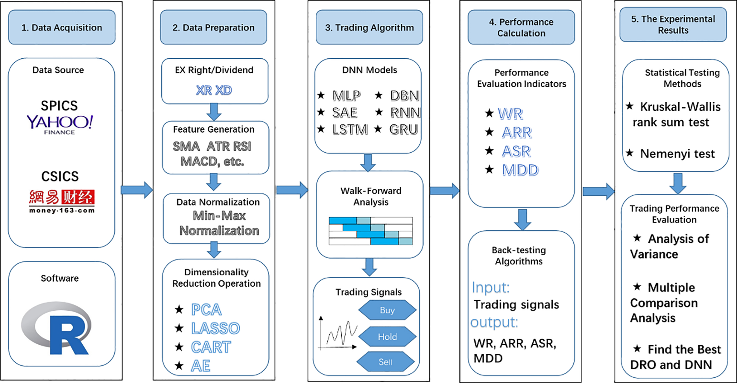

4. Data acquisition

4.1 Data source

In order to test the performance difference between any two trading algorithms on the large-scale datasets, we conduct experiments on the US SPICS and the Chinese CSICS, which represent the industry development of the world’s top two economies and are attractive to investors around the world. The reason for our choice of SPICS is that it includes a wide range of industries such as high-tech stocks, public utility stocks, and financial stocks, which account for more than 80% of the total market value of the US stock. These stocks have strong liquidity and can provide good objects for back-testing of trading strategies. Meanwhile, the selection criteria of CSICS are market value and liquidity, which accounts for more than 60% of the total market value of Chinese A-share listed companies. It is worth noting that whether the SPICS or CSICS is dynamically adjusted according to certain rules. Therefore, the stock that does not meet the requirements in a certain period will be removed from the original sample. In the experiments, we select the data from the past 2000 trading days of SPICS and CSICS before December 31, 2017, respectively. In order to get enough data for the experiments, we have removed the stocks that have been suspended, delisted, and less than 2000 trading days. Finally, we select 424 SPICS and 185 CSICS, which account for about 85% and 60% of the total number of stocks, respectively. Stocks are fewer in CSICS because the CSICS is adjusted once a year and their selection rules are more stringent.

We obtain the stock data of SPICS and CSICS from http://finance.yahoo.com and CSICS from http://quotes.money.163.com, respectively.

4.2 Software

All processes, from data acquisition, data preprocessing, feature generation, DRO, and DNN algorithms to trading performance measurement, are done used in R language (R version 3.4.3). R language is a statistical computing tool, which is widely used in the fields of statistical analysis, bioinformatics, financial modeling, machine learning and so on. We use quantmod-packet to obtain stock original data from relevant websites and use xts-package and TTR-packet to do data preprocessing and feature generation. we use glmnet-package, psych package, autoencoder-package, and rpart-packet to do DRO. We apply rnn-package and deepnet-package to train DNN models to generate trading signals. We use PerformanceAnalytics-package and pgirmess-package to evaluate the performance of the trading algorithms. All processes are carried out in the Window10 system (8 G memory, CPU frequency 2.81 Hz).

5. Data preparation

5.1 EX-rights/dividend

The data that we downloaded from the Internet include the trading time, the opening price, highest price, the lowest price, the closing price, and the volume. These data reflect the changes of stock price and volume of trading day. The acquired data is not processed by ex-dividend/weight, and we need to process these data accordingly. Because rationed shares, increasing shares by transferring and dividends can cause excessive jump and distortion of and technical indicators, which will affect the performance of trading algorithms.

5.2 Feature generation

In this paper, we select 44 relatively well-recognized technical indicators with a high frequency of use as the features, which include trend indicators, volatility indicators, cash flow indicators, investor psychological indicators and so on. The reason for choosing these indicators is that they describe the dynamic changes of stock price and volume in a trading day. It is worth noting that the number of technical indicators of stocks is large and the same indicator can generate many different indicators with the different parameters. In addition to some common indicators such as commodity channel index (CCI), relative strength index (RSI), there are some other indicators such as average true range (ATR), triple exponentially smoothed moving average (TRIX), because these indicators are of great significance for the characterizing the movement pattern of stock.

5.3 Data normalization

Data normalization is an important step in data preprocessing. Normalized data are generally used as inputs to machine learning and data mining models. The significance of normalization is to compress every feature in the data sets to the range of [0,1]. In this way, larger value of features can be avoided to have a strong influence on the output of the ML model, so as to improve the robustness of the model. In this article, we adopt max-min normalization. That is, to each feature $x$ , $x^{\ast}=({x-\max(x)})/({\max(x)-\max(x)})$ .

5.4 DRO algorithms

DRO tries to retain the information contained in the original features while minimizing the number of features. The purpose of DRO is to use a few features to replace the original large number of features for the training of ML models, which can improve the training efficiency of the models, reduce the impact of the redundant features on the model parameter estimation, and improve the robustness and generalization ability of the models. In engineering practice, we often obtain features of the research object as many as possible based on some priori knowledge of practical problems. However, some problems caused by too many features are that some features have nothing to do with the model and there exists multi-collinearity between features. Meanwhile, too many features increase the complexity of the models while reducing the explanatory power of the models. In this part, we mainly use four DRO algorithms (PCA, LASSO, CART, AE) to implement DRO for the original data, where PCA and AE are unsupervised DRO methods while CART and LASSO are supervised DRO methods. Then, we take the features after the DRO as the inputs of the DNN models.

Given a training dataset, $D=\{{({x_{1},y_{1}}),({x_{2},y_{2}}),\ldots,({x_{P},y_{P}})}\}$ , where $x_{i}=\{{x_{i1},x_{i2},\ldots,x_{iP}}\}$ is the $i$ -th sample of input; $P$ is the number of sample features; $y_{i}=\{{0,1}\}$ is the $i$ -th class label; $i=1,2,3,\ldots,N$ , where $N$ is the sample size $D$ is a matrix of $N\ast({P+1})$ , where the $P+1-th$ column of $D$ are class labels.

5.4.1 PCA

PCA [51] is to transform $P$ correlated original variables $x_{1},x_{2},\ldots,x_{P}$ into $M$ new unrelated variables through a linear transformation. That is, $Z_{m}=\sum_{j=1}^{P}{\varphi_{jm}x_{j}}$ , where $\varphi_{1m},\varphi_{2m},\ldots\varphi_{Pm}$ are constants, $m=1,2,\ldots,M$ . The least-square method can be used to fit the linear regression model, $y_{i}=\theta_{0}+\sum_{m=1}^{M}{\theta_{m}Z_{im}+\varepsilon_{i}}$ . The regression coefficients are $\theta_{0},\theta_{1},\ldots,\theta_{M}$ ; $\varepsilon_{i}$ is a normal distribution with the mean value is 0 and variance is 1. If the constants $\varphi_{1m},\varphi_{2m},\ldots\varphi_{Pm}$ are carefully chosen, such a DRO method will get better results than the ordinary least-square method. Here, the significance of DRO is to transform the $P+1$ variables that need to be estimated into $M+1$ variables, where $M\leqslant P$ . The purpose of the PCA is to transform the $P$ variables of the original dataset into $M$ orthogonal variables. These new variables, which are from large to small according to the variance, are called the first principal component and the second principal component and so on. Therefore, PCA can retain most of the information in original variables, reduce the number of variables, and achieve the purpose of DRO. In this paper, we use the correlation matrix of the features as the inputs of PCA and then examine the “scree” plot of the successive eigenvalues of the matrix to determine the number of factors or components.

5.4.2 LASSO

In order to prevent overfitting, LASSO regression is introduced to select variables in the least- square regression [51]. The constraint of the coefficient in empirical loss term is $\sum_{j=1}^{P}{|{\beta_{j}}|\leqslant s}$ . That is, solving $\beta_{j},j=0,1,\ldots,P;\lambda$ to make $\sum_{i=1}^{N}{({y_{i}-\beta_{0}-\sum_{j=1}^{P}{\beta_{j}x_{ij}}})}^{2}+% \lambda\sum_{j=1}^{P}{|{\beta_{j}}|}$ minimization. LASSO compresses the estimated value of the coefficient in the direction of 0. Furthermore, when the adjustment parameter $\lambda$ is a large enough, the added penalty term has the effect of forcing the estimated value of some of the coefficients to be 0. Therefore, adjusting the relationship between $\beta_{j},j=0,1,\ldots,P$ and $\lambda$ can realize the function of DRO. In this paper, we use grid search and cross-validation to find the best $\lambda$ , then obtain the variables that coefficients are not 0 are the features we want.

5.4.3 CART

CART [51] is a prediction model of attribute structure and represents a mapping relationship between attributes of an object and value of the object. The CART includes a root node, a series of tree branches, and multiple leaf nodes. In training process of the CART algorithm, which attribute is chosen as its root node and which node to choose as its next node are determined by the importance of the information represented by the attribute for the classification results. The method of measuring the importance of attributes is also a method of DRO. The CART uses Gini coefficient to measure the contribution of an attribute to classification. The degree of importance of a feature or attribute is determined by the degree of reduction in the classification uncertainty. In CART, Gini coefficient is the degree of uncertainty in the classification of datasets under given certain features. Different features often have different Gini coefficients. The smaller the Gini coefficient, the stronger the classification ability. The Gini coefficient is widely used in the classification tree, regression tree, and random forest algorithm.

5.4.4 AE

AE [52] is a kind of feed-forward neural network, which can be used for data DRO. It is a neural network with a single hidden layer. That is, the network structure consists of an input layer, an output layer, and a hidden layer. The number of neuron in the hidden layer is less than that of the input layer. By minimizing the mean square error between the inputs and outputs, the inputs are reconstructed by the outputs so as to reduce the dimension of the original inputs. AE is an unsupervised DRO method and deal with original features through nonlinear transformation, so it can learn the information of original features. The method is mainly used in the fields of image generation, pattern recognition and so on. In this paper, we choose 10 neurons in the hidden layer. That is, we select the number of variables to be 10 in each DRO process.

5.4.5 Summary of the DRO

Different DRO has its advantages and limitations because of different mathematical principles. Meanwhile, the validity of DRO depends on the characteristics of data. In this paper, we present two unsupervised DRO (PCA and AE). PCA extracts principal components by a linear combination of features and determines the number of features after DRO by cumulative contribution rate. AE specifies the number of features after DRO artificially by a non-linear mapping relationship between features. Both CART and LASSO are supervised DRO. That is, there is a dependency relationship between features and classification labels when DRO is performed. CART chooses features by evaluating the importance of features based on Gini coefficient; LASSO compresses the coefficients of variables that are not important relative to label to be 0, thus realizing DRO. The advantages and limitations of these four methods are shown in Table 1.

Table 1
A summary of advantages and limitations of the DRO

	Advantage	Limitation
PCA	PCA measures information of features by variance and it is not restricted by labels. The features after dimension reduction are linearly independent, which can eliminate the multi-collinearity between features. The calculation method of PCA is simple and easy to implement.	In PCA, a basic requirement is that the cumulative contribution rate of a few principal components can reach a higher level. Secondly, the extracted principal components lack meaningful explanations.
CART	CART can clearly show which features are important and which features are not important. Meanwhile, CART can deal with continuous and discrete features. In the process of dimension reduction, CART does not need any domain knowledge and assumption of parameters. It is very suitable for dimensionality reduction of high-dimensional data. Its calculation speed is very fast.	When the features selected by CART are used as input of other machine learning algorithms, these algorithms are prone to be over-fitting. Moreover, CART only considers the relationship between features and labels when considering the importance of features, but ignores the relationship between features.
LASSO	LASSO is a supervised dimensionality reduction method. If there are noise and redundancy in data, LASSO can find useful features and reduce redundancy, so that improve the accuracy and robustness of algorithms.	LASSO is not applicable when features are not sparse. Meanwhile, the coefficients selected by LASSO are biased.
AE	AE can capture the non-linear relationship between features. It can reduce the number of original features according to the need of special problem while retaining the information of the original features completely.	The number of features chosen by AE has strong subjectivity. The speed of AE is slow. The feature selection process of AE is unsupervised. The accuracy of AE depends on the amount of data.

6. Algorithm for generating trading signals and trading strategy

6.1 DNN models

The task of us is to construct a DNN model based on a given training dataset after DRO so that the model can predict the directions of stock price movement correctly. In this paper, in order to test whether the DRO can improve the trading performance of the DNN algorithms, we apply the widely used PCA, LASSO, CART, and AE to be the DRO algorithm to deal with the original input features respectively, then use a DNN model such as MLP [53], DBN [54], SAE [55], RNN [56], LSTM [56], and GRU [56] as classifier to predict the rising and falling of the stock prices. The main model parameters and training parameters of these DNN algorithms are shown in Table 2.

In Table 2, features and class labels are set according to the input format of various DNN algorithms in R language. Matrix ( $m$ , $n$ ) represents a matrix with $m$ rows and $n$ columns; Array ( $q$ , $m$ , $n$ ) represents a tensor (namely array in R language), where each layer of the tensor is Matrix ( $m$ , $n$ ) and the height of the tensor is $q$ . $c$ (h1, h2, h3, $\ldots$ ) represents a vector, where the length of the vector is the number of hidden layer and the $i$ -th element of $c$ is the number of neuron of the $i$ -th layer. In the experiment, $m=$ 250 represents that the data of the past 250 days (about 250 trading days in a year) is used as training samples in each round of WFA; $n=p$ represents that there are $p$ features after DRO. In Table 2, the activation function of all DNN models is a sigmoid function. Other parameters such as learning rate, batch size, and epoch are all the default values in the DNN algorithms of R programs.

Table 2
Parameter settings of DNN models

	Input	Label	Learning rate	Dimensions of hidden layers	Activation function	Batch size	Epoch
MLP	Matrix(250,p)	Matrix(250,1)	0.80	c(25,15,10,5)	Sigmoid	100	3
DBN	Matrix(250,p)	Matrix(250,1)	0.80	c(25,15,10,5)	Sigmoid	100	3
SAE	Matrix(250,p)	Matrix(250,1)	0.80	c(20,10,5)	Sigmoid	100	3
RNN	Array(1,250,p)	Array(1,250,1)	0.01	c(10,5)	Sigmoid	1	1
LSTM	Array(1,250,p)	Array(1,250,1)	0.01	c(10,5)	Sigmoid	1	1
GRU	Array(1,250,p)	Array(1,250,1)	0.01	c(10,5)	Sigmoid	1	1

Figure 2.

The schematic diagram of WFA.

6.2 Walk-forward analysis

WFA [57] is a systematic manner of performing what has been referred to as a rolling training and testing (see Fig. 2). One of the primary strengths of the WFA is to determine the robustness of the trading strategy. WFA is to determine the degree of confidence with which the trader may anticipate that the strategy will perform in real-time trading. Another important advantage of WFA is to produce a better trading performance as market changes. Since this periodic re-optimization is done with a strategy-appropriate amount of current price data, which also provides an efficient way to continuously adapt a trading model to ongoing changes in market conditions.

In this paper, we use DNN algorithms and WFA method to predict the stock price trends as trading signals. In each step, we first apply a DRO algorithm to handle raw input data which is from the past 250 days (one year), then apply the new dataset after DRO as the training set to train DNN models. Finally, we use the data of the next 5 days (one week) as the test set to predict the directions of the stock prices. It is worth noting that the features may be different (such as p1, p2, $\ldots$ , pn (max (p1, p2, $\ldots$ , pn) $<=$ 44) are shown in Fig. 2) after each round of DRO, so the parameters of the DNN models will be different in each round of training. Therefore, the trained models are more likely to adapt to the current market conditions and the prediction results are more robust. Each stock contains data for 2,000 trading days, so it takes (2000–250)/5 $=$ 350 training sessions to produce a total of 1,750 predictions which are the trading signals of daily trading strategy. The WFA method is shown in Fig. 2.

6.3 The algorithm for generating trading signals

In this part, we use DNN algorithms as the classifiers to predict the ups and downs of the stock both in the SPICS and CSICS. Then, we apply the prediction results as trading signals of daily trading. In this process, we use the WFA method to train each DNN algorithm and to test out-of-sample data. We give the generating algorithm of trading signals according to Fig. 2, as is shown in Algorithm 1.

Algorithm 1. Generating Trading Signals in R Language
Input: Stock Symbols List
Output: Trading Signals
1. $N=$ Length of Stock Symbols List # $N=$ 424 in SPICS and 185 in CSICS 2. $L=$ Number of Samples # $L=$ 2000 3. $P=$ Length of Features # $P=$ 44 4. $k=$ Length of Training Dataset # $k=$ 250 5. $n=$ Length of Testing Dataset or Length of WFA Window # $n=$ 5 6. for (i in 1:N){ 7. Stock Data $=$ Stock Symbol List[i] #train sets 8. M $=$ (L-k)/n 9. Trading Signal $=$ NULL 10. for (j in 1:M) { 11. Raw_Data $=$ Stock Data[( $k+n(j-1)$ ):( $k+n+n(j-1))$ , 1:( $P+1$ )] 12. New_Data $=$ DRO Algorithm (Raw_Data) 13. New_Train $=$ New_Data[1:k,] 14. New_Test $=$ New_Data[( $k+1$ ): ( $k+n$ )],1:p]# $p\leqslant P$ 15. Train_Model $=$ DNN Model(New_Train) 16. Proba $=$ Train_Model(New_Test) 17. if (Proba $\geqslant$ 0.5) { 18. Trading Signal0 $=$ 1 19. } else { 20. Trading Signal0 $=$ 0 21. } 22. Trading Signal $=$ c(Trading Signal, Trading Signal0) 23. } 24. return (Trading Signals)

Algorithm 1. Generating Trading Signals in R Language

Input: Stock Symbols List

Output: Trading Signals

1.
$N=$ Length of Stock Symbols List # $N=$ 424 in SPICS and 185 in CSICS 2.
$L=$ Number of Samples # $L=$ 2000
3.
$P=$ Length of Features # $P=$ 44
4.
$k=$ Length of Training Dataset # $k=$ 250
5.
$n=$ Length of Testing Dataset or Length of WFA Window # $n=$ 5
6.
for (i in 1:N){
7.
Stock Data $=$ Stock Symbol List[i] #train sets
8.
M $=$ (L-k)/n
9.
Trading Signal $=$ NULL
10.
for (j in 1:M) {
11.
Raw_Data $=$ Stock Data[( $k+n(j-1)$ ):( $k+n+n(j-1))$ , 1:( $P+1$ )]
12.
New_Data $=$ DRO Algorithm (Raw_Data)
13.
New_Train $=$ New_Data[1:k,]
14.
New_Test $=$ New_Data[( $k+1$ ): ( $k+n$ )],1:p]# $p\leqslant P$
15.
Train_Model $=$ DNN Model(New_Train)
16.
Proba $=$ Train_Model(New_Test)
17.
if (Proba $\geqslant$ 0.5) {
18.
Trading Signal0 $=$ 1
19.
} else {
20.
Trading Signal0 $=$ 0
21.
}
22.
Trading Signal $=$ c(Trading Signal, Trading Signal0)
23.
}
24.
return (Trading Signals)

6.4 Trading strategy

In this section, we give a daily trading strategy. If our DNN model predicts that a stock price of the next day will rise, then we will buy the stock at today’s closing price and sell it at the next day’s closing price. If our DNN model predicts that a stock price of the next day will fall, then we do not implement to buy or sell operation. That is, our strategy does not allow short selling. Therefore, the holding period of stock is one day. In our daily trading strategy, the implicit assumption is that we can complete the stock trading at the closing price. We know that this is very difficult in real trading, but it is entirely possible to do it near the closing price such as the trading price deviates from the closing price of 0.01 or 1 tick. Meanwhile, we do not consider trading cost in our strategy. In fact, it is very simple to consider trading cost in the strategy. Because whether in the U.S. stock market or China’s A-share market, the transparent transaction costs (broker commissions, exchange fees, and taxes) account for only a small part of stock investment returns. Our trading frequency is not particularly high, even may only trade once every few days.

7. The experimental results

7.1 Trading performance measure indicators

Investment performance measurement is an important tool to evaluate the effectiveness of a quantitative trading algorithm or trading strategy. In this paper, we apply the WR [38], ARR [38], ASR [38], MDD, and ATT as the measurement indicators of the trading performance. These indicators reflect the investment ability of investors or the performance of trading algorithms.

Drawdown is a measure of historical loss. It is the largest loss compared to the previous highest value (water level) of the net value curve and helps illustrate potential downside risk. Investment managers usually get performance reward after their investment returns exceed the water level MDD records the lowest peak-to-trough return from the last global maximum to the minimum that occurred prior to the next global maximum that supersedes the last global maximum MDD shows the largest decline in the price or value of the investment period $H$ , which is an important risk assessment indicator. In the period of investment $t$ , we first calculate the $D_{t}$ at any time $t\leqslant H$ . Then we can get the $\textit{MDD}_{H}$ when we go traverse the whole interval.

$\displaystyle{D}_{t}{=}\mathop{\max P_{t_{1}}}\limits_{t_{1}\in\left[{0,t}% \right]}-\mathop{\min P_{t_{1}}}\limits_{t_{2}\in\left[{0,t}\right]}|\forall t% _{1}<t_{2};\textit{MDD}_{H}=\mathop{\max D_{t}}\limits_{t\in\left[{0,H}\right]% }/\mathop{\max P_{t}}\limits_{t\in\left[{0,H}\right]}$

where $P_{t}$ denotes the value of the net value curve with time $t$ ; $D_{t}$ represents the drawdown at the time $t$ . $\textit{MDD}_{H}$ denotes the maximum drawdown in $\left[{0,H}\right]$ .

ATT is an average training time for a DNN algorithm to generate the trading signals of individual stock, which is an important performance measure indicator of the trading algorithm. The training speed of the algorithm is very important in daily trading because it must generate the trading signal for the next trading day near the closing price of the trading day so that we can make fast and effective investment decisions. In particular, ATT is a very important consideration when the trading algorithm is used in intraday trading or high-frequency trading because capturing the fleeting trading opportunities is the key to profitability. In this paper, we use second(s) as the unit of time.

7.2 Non-parameter statistical test method

In this paper, we study the impact of the DNN algorithms based on different DRO on the trading performance both in SPICS and CSICS. We will implement experiments on 24 trading algorithms, which based on 6 DNN and 4 DRO. The 4 DRO often serve as the important choice for high dimensional data preprocessing in other applications and these DRO usually greatly improve the computational efficiency while losing some information. Next, we mainly test the performance of these algorithms in the two datasets to evaluate whether there are significant differences between a DNN algorithm after the different DRO methods and whether there is a significant difference between the performance of the DNN algorithm after DRO and that of the DNN algorithm itself. Therefore, we use statistical hypothesis testing to compare and analyze the trading performance of different algorithms.

The statistical hypothesis testing uses sample information to reject or accept the distribution hypothesis based on a certain probability. For example, when we test whether there are significant differences between the mean values of two or more populations, we first take a certain number of samples from different populations so that the sample mean is a statistic of the population mean. We assume that the difference between the sample mean and the population mean comes from sampling error. If the value of the sample statistic falls within the region where the probability of occurrence is large in the sampling distribution, we believe that there is no significant difference between the sample mean and the population mean; if this sample statistic falls within the region where the probability of occurrence is very small in the sampling distribution, the researchers have to admit the difference between the sample mean and the population mean based on the principle that small probability event is almost impossible to occur in a random sample. The difference is not caused by sampling errors, but by an essential difference between them. Based on the above theoretical analysis, we propose the following hypotheses of the problems concerned in this paper: Given a DNN algorithm $i\in\left\{{\textit{MLP},\textit{DBN},\textit{SAE},\textit{RNN},\textit{LSTM},% \textit{GRU}}\right\}$ ; Given a performance measure indicator $j\in\left\{{\textit{WR},\textit{ARR},\textit{ASR},\textit{MDD},\textit{ATT}}\right\}$ ; for any DRO algorithm $k\in\left\{{\textit{LASSO},\textit{PCA},\textit{CART},\textit{AE}}\right\}$ . We propose the following basic hypotheses for significance testing in which Hijka are the null hypothesis, and the corresponding alternative hypotheses are Hijkb. The level of significance is 0.05. That is, the probability of rejecting the null hypothesis is 5%.

Hijka: Given a DNN algorithm $i$ , all DRO $k$ based on the algorithm $i$ are the same on a given measurement indicator $j$ ; That is to say, there is no significant difference between mean of trading performance of all algorithms.

Hijkb: Given a DNN algorithm $i$ , all DRO $k$ based on the algorithm $i$ are not the same on a given measurement index $j$ ; That is to say, there is a significant difference between mean of trading performance of all algorithms.

For example, $i=$ MLP, $j=$ WR, we have the following statistical test hypothesis:

Hijka: the WR of MLP, MLP $+$ LASSO, MLP $+$ PCA, MLP $+$ CART, MLP $+$ AE are the same; Hijkb: the WR of MLP, MLP $+$ LASSO, MLP $+$ PCA, MLP $+$ CART, MLP $+$ AE are not the same.

In statistical hypothesis testing, statistics and their probability in sampling distribution are generally calculated from the null hypothesis. The judgment of rejecting the null hypothesis or accepting the null hypothesis is made according to the comparison between the probability and the significance level. If the probability is less than 0.05, this means that a small probability event has occurred. That is, we have found the reason for rejecting the null hypothesis with a minimum probability of making a mistake. Otherwise, there is not enough reason to reject the null hypothesis.

It is worth noting that any performance measure indicator of all trading algorithms or strategies does not conform to the basic hypothesis of variance analysis in our previous research work. Therefore, it is not appropriate to use t-test in the analysis of variance. And we should take the non-parametric statistical test method. In this paper, we use the Kruskal-Wallis rank sum test [59] to implement the analysis of variance. If the alternative hypothesis is established, we need to apply the Nemenyi test [60] further to do the multiple comparisons between the performance of trading algorithms.

7.3 Comparative analysis of the performance between different trading algorithms in SPICS

We give the average value of each performance measure indicator of each DNN after DRO by implementing back-testing. Then we analyze in detail whether the DRO can improve the trading performance of the DNN algorithm and whether there are statistically significant differences between the trading performance of a DNN algorithm based on different DRO.

Table 3
Performance of MLP based on different DRO methods. Best performance of all trading algorithms is in bold font

	WR	ARR	ASR	MDD	ATT
MLP	0.5676	0.3333	1.5472	0.3584	0.02s
MLP $+$ LASSO	0.5660	0.3262	1.5131	0.3618	0.62s
MLP $+$ PCA	0.5665	0.3279	1.5250	0.3592	0.38s
MLP $+$ CART	0.5664	0.3263	1.5163	0.3615	0.03s
MLP $+$ AE	0.5666	0.3275	1.5252	0.3588	2.76s

We can see from Table 3 that the performance (WR, ARR, ASR, MDD, and ATT) of MLP is better that of other algorithms. Through the analysis of variance and multiple comparisons, we can find that there is no significant difference between the performance of all trading algorithms. The ATT of MLP is significantly less than those of other algorithms. Therefore, any DRO cannot improve the performance of MLP. Meanwhile, the performance of MLP after different DRO has no significant difference except for ATT.

Table 4

Performance of DBN based on different DRO methods. Best performance of all trading algorithms is in bold font

	WR	ARR	ASR	MDD	ATT
DBN	0.5680	0.3298	1.5415	0.3585	0.17s
DBN $+$ LASSO	0.5680	0.3285	1.5441	0.3520	1.56s
DBN $+$ PCA	0.5673	0.3293	1.5374	0.3568	0.87s
DBN $+$ CART	0.5671	0.3281	1.5330	0.3559	0.17s
DBN $+$ AE	0.5695	0.3308	1.5924	0.3661	9.63s

We can see from Table 4 that the WR, ARR, and ASR of DBN $+$ AE are the greatest in all algorithms. The MDD of DBN $+$ LASSO is the smallest in all algorithms. The ATT of DBN and DBN $+$ CART are smaller than those of other algorithms. Through the analysis of variance and multiple comparisons. There is no significant difference between the performance measure indicators (WR, ARR, ASR, and MDD) of all trading algorithms. The ATT of DBN and DBN $+$ CART have no significant difference, but they are significantly smaller those of other algorithms. Therefore, any DRO cannot significantly improve the performance of DBN. Meanwhile, the execution speed of CART is significantly faster than those of other DRO.

Table 5

Performance of SAE based on different DRO methods. Best performance of all trading algorithms is in bold font

	WR	ARR	ASR	MDD	ATT
SAE	0.5683	0.3327	1.5506	0.3547	0.05s
SAE $+$ LASSO	0.5673	0.3274	1.5382	0.3493	0.72s
SAE $+$ PCA	0.5670	0.3263	1.5249	0.3593	0.81s
SAE $+$ CART	0.5669	0.3272	1.5305	0.3580	0.04s
SAE $+$ AE	0.5671	0.3271	1.5261	0.3597	9.26s

We can see from Table 5 that the performance measure indicator (WR, ARR, and ASR) of SAE is the best in all algorithms; the MDD of SAE $+$ LASSO is the smallest in all algorithms; the ATT of SAE $+$ CART is the smallest in all algorithms. Through the analysis of variance and multiple comparisons, there is no significant difference between any performance measure indicator (WR, ARR, ASR, and MDD) of all trading algorithms. The ATT of SAE and SAE $+$ CART have no significant difference, but they are significantly smaller those of other algorithms. Therefore, any DRO cannot significantly improve the performance of SAE. Meanwhile, there is no significant difference between any two DRO for the performance (WR, ARR, and ASR) of SAE.

Table 6

Performance of RNN based on different DRO methods. Best performance of all trading algorithms is in bold font

	WR	ARR	ASR	MDD	ATT
RNN	0.5843	0.2945	1.5768	0.3403	0.01s
RNN $+$ LASSO	0.8349	0.2333	2.5708	0.1270	0.72s
RNN $+$ PCA	0.5231	0.0846	0.4735	0.3599	0.36s
RNN $+$ CART	0.5235	0.0816	0.4692	0.3594	0.02s
RNN $+$ AE	0.5817	0.2953	1.5652	0.3475	8.26s

We can see from Table 6 that the WR, ASR, and MDD of RNN $+$ LASSO are better than those of other algorithms, respectively; the ARR of RNN $+$ AE is the greatest in all algorithms; the ATT of RNN is smaller than those of other algorithms. Through the analysis of variance and multiple comparisons, the WR of RNN $+$ LASSO is significantly greater than those of other algorithms; the WR of RNN $+$ AE is significantly greater than those of RNN $+$ PCA and RNN $+$ CART, but is not significantly different from that of RNN. The ARR of RNN and RNN $+$ AE have no significant difference, but they are significantly greater than those of other algorithms. The ASR of RNN $+$ LASSO is significantly greater than those of other algorithms; the ASR of RNN and RNN $+$ AE have no significant difference, but they are significantly greater than those of RNN $+$ PCA and RNN $+$ CART. The MDD of RNN $+$ LASSO is significantly smaller than those of other algorithms, and the MDD of all algorithms have no significant difference except RNN $+$ LASSO. The ATT of RNN and RNN $+$ CART have no significant difference, but they are significantly smaller than those of other algorithms. Therefore, LASSO can significantly improve the performance (WR, ASR, and MDD) of RNN. In addition, other DRO cannot significantly improve the performance of RNN, even CART and PCA can make the performance of RNN worse.

Table 7

Performance of GRU based on different DRO methods. Best performance of all trading algorithms is in bold font

	WR	ARR	ASR	MDD	ATT
GRU	0.5844	0.2935	1.5832	0.3381	0.10s
GRU $+$ LASSO	0.5640	0.3310	1.4753	0.3891	0.40s
GRU $+$ PCA	0.5234	0.0814	0.4683	0.3617	0.55s
GRU $+$ CART	0.5240	0.0821	0.4763	0.3558	0.19s
GRU $+$ AE	0.5859	0.2912	1.5848	0.3422	3.62s

We can see from Table 7 that the WR and ASR of GRU $+$ AE is the greatest in all algorithms, respectively; the ARR of GRU $+$ LASSO is the greatest in all algorithms; the MDD and ATT of GRU is smaller than those of other algorithms, respectively. Through the analysis of variance and multiple comparisons, there is no significant difference between the WR of GRU $+$ AE and GRU; the WR of GRU is significantly greater than those of GRU $+$ CART and GRU $+$ PCA. The ARR of GRU $+$ LASSO is significantly greater than those of other algorithms; the ARR of GRU and GRU $+$ AE have no significant difference, but they are significantly better than those of GRU $+$ PCA and GRU $+$ CART. The ASR of GRU, GRU $+$ LASSO, and GRU $+$ AE have no significant difference, but they are significantly greater than those of GRU $+$ PCA and GRU $+$ CART. The MDD of all algorithms have no significant difference expect GRU $+$ LASSO, but the MDD of GRU is significantly smaller than that of GRU $+$ LASSO. The ATT of GRU is significantly smaller than those of other algorithms. Therefore, LASSO can significantly improve the ARR of GRU. In addition, any DRO cannot do this.

Table 8

Performance of LSTM based on different DRO methods. Best performance of all trading algorithms is in bold font

	WR	ARR	ASR	MDD	ATT
LSTM	0.5825	0.2921	1.5575	0.3489	0.11s
LSTM $+$ LASSO	0.5681	0.3647	1.6233	0.3564	0.88s
LSTM $+$ PCA	0.5231	0.0812	0.4672	0.3536	0.42s
LSTM $+$ CART	0.5240	0.0870	0.4984	0.3546	0.21s
LSTM $+$ AE	0.5863	0.2884	1.5786	0.3467	5.53s

We can see from Table 8 that the WR and MDD of LSTM $+$ AE is the best in all trading algorithms, respectively; the ARR and ASR of LSTM $+$ LASSO is the greatest in all algorithms, respectively; the ATT of LSTM is smaller than those of other algorithms. Through the analysis of variance and multiple comparisons, the WR of LSTM is significantly greater than those of LSTM $+$ PCA, LSTM $+$ CART, and LSTM $+$ LASSO, but is not significantly different from that of LSTM $+$ AE; the ARR of LSTM $+$ LASSO is significantly greater than those of other algorithms; the ARR of LSTM is significantly greater than those of LSTM $+$ PCA and LSTM $+$ CART, but is not significantly different from that of LSTM $+$ AE. The ASR of LSTM, LSTM $+$ LASSO, and LSTM $+$ AE have no significant difference, but they are significantly greater than those of other algorithms. The MDD of all algorithms have no significant difference. The ATT of LSTM is significantly smaller than those of other algorithms. Therefore, LASSO can significantly improve ARR of LSTM. In addition, any DRO cannot do this.

By means of variance analysis and multiple comparison methods, the experimental results can be found as follows. From the perspective of forecasting accuracy of trading signals, we can see that LASSO can significantly improve the WR of RNN; in addition, any DRO cannot improve the WR of the remaining five DNN models. From the perspective of annual average returns, LASSO can significantly improve the ARR of GRU and LSTM; in addition, any DRO cannot improve the RNN of the remaining four DNN models. From the perspective of risk-adjusted returns, LASSO can significantly improve the ASR of RNN; in addition, any DRO cannot significantly improve the ASR of the remaining five DNN models. From the perspective of trading risk control, LASSO can significantly improve the MDD of RNN; in addition, any DRO cannot significantly improve the MDD of the remaining five DNN models. From the perspective of the speed of the trading signals generated by the algorithms, the ATT of all DNN algorithms are not significantly slower than those of the fastest algorithms based on DRO methods. That is, any DRO cannot significantly improve the execution speed of any DNN models.

7.4 Comparative analysis of the performance between different trading algorithms in CSICS

Similar to 7.3, we give the average value of each performance measure indicator of each DNN model and the model after DRO. Then we apply variance analysis and multiple comparison methods to analyze whether DRO can improve the performance and execution speed of the DNN models.

Table 9
Performance of MLP based on different DRO methods. Best performance of all trading algorithms is in bold font

	WR	ARR	ASR	MDD	ATT
MLP	0.5559	0.5731	1.4031	0.6082	0.02s
MLP $+$ LASSO	0.5556	0.5762	1.4039	0.6070	2.07s
MLP $+$ PCA	0.5555	0.5712	1.3966	0.6110	0.84s
MLP $+$ CART	0.5558	0.5719	1.3976	0.6119	0.09s
MLP $+$ AE	0.5558	0.5733	1.4024	0.6073	10.97s

From Table 9, we can see that the WR of MLP is the greatest; the ARR, ASR, and MDD of MLP $+$ LASSO is the best in all algorithms, respectively; the ATT of MLP is the smallest in all trading algorithms. Through variance analysis and multiple comparison methods, we can find that the performance (WR, ARR, ASR, and MDD) of MLP and that of the model after DRO have no significant difference, but the ATT of MLP is significantly smaller than those of other algorithms. Therefore, any DRO cannot significantly improve the performance of MLP. Meanwhile, DRO can reduce the execution speed of MLP.

Table 10

Performance of DBN based on different DRO methods. Best performance of all trading algorithms is in bold font

	WR	ARR	ASR	MDD	ATT
DBN	0.5565	0.5704	1.4006	0.6086	0.08s
DBN $+$ LASSO	0.5574	0.5759	1.4159	0.6070	0.89s
DBN $+$ PCA	0.5562	0.5713	1.3997	0.6136	0.51s
DBN $+$ CART	0.5563	0.5711	1.4017	0.6109	0.08s
DBN $+$ AE	0.5560	0.5722	1.4058	0.6088	8.23s

From Table 10, we can see that the performance (WR, ARR, ASR, and MDD) of DBN $+$ LASSO is the best in all algorithms, respectively; the ATT of DBN $+$ CART and DBN is the smallest in all trading algorithms, respectively. Through variance analysis and multiple comparison methods, we can find that the performance (WR, ARR, ASR, and MDD) of DBN and the model after DRO have no significant difference. The ATT of DBN and DBN $+$ CART have no significant difference, but they are significantly smaller than those of other trading algorithms. Therefore, any DRO cannot significantly improve the performance of DBN. Meanwhile, any DRO cannot significantly accelerate the execution speed of DBN.

Table 11

Performance of SAE based on different DRO methods. Best performance of all trading algorithms is in bold font

	WR	ARR	ASR	MDD	ATT
SAE	0.5564	0.5678	1.3935	0.6130	0.09s
SAE $+$ LASSO	0.5568	0.5710	1.4054	0.6081	0.84s
SAE $+$ PCA	0.5566	0.5732	1.4077	0.6077	0.62s
SAE $+$ CART	0.5563	0.5725	1.4046	0.6093	0.08s
SAE $+$ AE	0.5560	0.5667	1.3918	0.6161	7.23s

From Table 11, we can see that the WR of SAE $+$ LASSO is the greatest in all trading algorithms; the ARR, ASR, and MDD of SAE $+$ PCA is the best in all algorithms, respectively; the ATT of SAE $+$ CART is the smallest in all trading algorithms. Through variance analysis and multiple comparison methods, we can find that the performance of SAE and the model after DRO have no significant difference; the ATT of SAE $+$ CART is not significantly different from that of the SAE, but they are significantly smaller than those of other algorithms Therefore, any DRO cannot significantly improve the performance of SAE. Meanwhile, any DRO cannot significantly accelerate the execution speed of SAE.

Table 12

Performance of RNN based on different DRO methods. Best performance of all trading algorithms is in bold font

	WR	ARR	ASR	MDD	ATT
RNN	0.5681	0.5248	1.4880	0.5648	0.08s
RNN $+$ LASSO	0.6045	0.4953	1.6637	0.5115	1.77s
RNN $+$ PCA	0.5095	0.1240	0.3370	0.6070	0.71s
RNN $+$ CART	0.5104	0.1313	0.3590	0.6077	0.09s
RNN $+$ AE	0.5714	0.5375	1.5455	0.5533	4.52s

From Table 12, we can see that the performance (WR, ASR, and MDD) of RNN $+$ LASSO is the best in all algorithms; the ARR of RNN $+$ AE is the greatest in all trading algorithms; the ATT of RNN is the smallest. Through variance analysis and multiple comparison methods, we can find that the WR of RNN is significantly smaller than that of RNN $+$ LASSO, but is significantly greater than those of RNN $+$ PCA and RNN $+$ CART. Meanwhile, the WR of RNN and RNN $+$ AE have no significant difference. The performance (ARR and ASR) of RNN is not significantly different from those of RNN $+$ LASSO and RNN $+$ AE, but is significantly greater than those of RNN $+$ PCA and RNN $+$ CART. The MDD of RNN is significantly greater than that of RNN $+$ LASSO, but is significantly smaller than those of RNN $+$ PCA and RNN $+$ CART. Meanwhile, the MDD of RNN and RNN $+$ AE have no significant difference. The ATT of RNN and RNN $+$ CART have no significant difference, but they are significantly smaller than those of other algorithms. Therefore, LASSO can significantly improve the WR and MDD of RNN. In addition, any DRO cannot significantly improve any performance measure indicator of RNN.

Table 13

Performance of GRU based on different DRO methods. Best performance of all trading algorithms is in bold font

Performance	WR	ARR	ASR	MDD	ATT
GRU	0.5717	0.5113	1.5505	0.5429	0.31s
GRU $+$ LASSO	0.6084	0.4719	1.7532	0.4794	1.77s
GRU $+$ PCA	0.5092	0.1152	0.3391	0.5815	1.05s
GRU $+$ CART	0.5090	0.1098	0.3218	0.5853	0.32s
GRU $+$ AE	0.5713	0.5179	1.5294	0.5484	3.12s

From Table 13, we can see that the performance (WR, ASR, and MDD) of GRU $+$ LASSO is the best in all algorithms; the ATT of GRU is the smallest in all algorithms. Through variance analysis and multiple comparison methods, we can find that the performance (WR, ASR and MDD) of GRU is significantly worse than that of GRU $+$ LASSO, but is significantly better than those of GRU $+$ PCA and GRU $+$ CART. Meanwhile, the WR of GRU and GRU $+$ AE have no significant difference. The ARR of GRU is not significantly different from those of GRU $+$ LASSO and GRU $+$ AE, but is significantly greater than those of GRU $+$ PCA and GRU $+$ CART. The ATT of GRU is not significantly different from that of GRU $+$ CART, but they are significantly smaller than those of other algorithms. Therefore, LASSO can significantly improve the WR, ASR and MDD of GRU. In addition, any DRO cannot significantly improve any performance measure indicator of GRU.

Table 14

Performance of LSTM based on different DRO methods. Best performance of all trading algorithms is in bold font

Performance	WR	ARR	ASR	MDD	ATT
LSTM	0.5720	0.5165	1.5422	0.5456	0.10s
LSTM $+$ LASSO	0.6196	0.4717	1.7355	0.4864	0.90s
LSTM $+$ PCA	0.5096	0.1221	0.3547	0.5777	0.40s
LSTM $+$ CART	0.5080	0.1098	0.3200	0.5916	0.23s
LSTM $+$ AE	0.5723	0.5197	1.5559	0.5410	5.68s

From Table 14, we can see that the performance (WR, ASR, and MDD) of LSTM $+$ LASSO is the best in all algorithms.; the ARR of LSTM $+$ AE is the greatest in all trading algorithms; the ATT of LSTM is the smallest. Through variance analysis and multiple comparison methods, we can find that the performance (WR and MDD) of LSTM is significantly worse than that of LSTM $+$ LASSO, but is significantly better than those of LSTM $+$ PCA and LSTM $+$ CART. Meanwhile, the performance (WR and MDD) of LSTM is not significantly different from that of LSTM $+$ AE. The ARR of LSTM is not significantly different from those of LSTM $+$ LASSO and LSTM $+$ AE, but is significantly greater than those of LSTM $+$ CART and LSTM $+$ PCA. The ASR of LSTM is not significantly different from those of LSTM $+$ LASSO and LSTM $+$ AE, but is significantly than those of LSTM $+$ CART and LSTM $+$ PCA. The ATT of LSTM is significantly less than those of other algorithms. Therefore, LASSO can significantly improve the WR and MDD of LSTM. In addition, any DRO cannot significantly improve any performance measure indicator of LSTM.

By means of variance analysis and multiple comparison methods, the experimental results on CSICS can be found as follows. From the perspective of forecasting accuracy of trading signals, we can see that LASSO can significantly improve the WR of RNN, LSTM, and GRU; in addition, any DRO cannot significantly improve the WR of the remaining DNN algorithms. From the perspective of annual average returns, any DRO cannot significantly improve the ARR of all DNN algorithms. From the perspective of risk-adjusted returns, LASSO can significantly improve the ASR of GRU; in addition, any DRO cannot significantly improve the ASR of other DNN algorithms. From the perspective of trading risk control, LASSO can significantly improve the MDD of RNN, GRU, and LSTM; in addition, any DRO cannot significantly improve the MDD of other DNN algorithms. From the perspective of the speed of the trading signals generated by the algorithms, the ATT of all DNN algorithms are not significantly slower than that of the algorithms after any DRO.

7.5 Discussions

From Sections 7.3 and 7.4, we can see that the DRO mentioned in this paper cannot significantly improve the trading performance (WR, ARR, ASR, and MDD) and the speed of generating trading signals of the MLP, SAE, and DBN both in SPICS and CSICS. This may be because the three DNN algorithms have the ability to automatically select the original features so that there is no significant difference between the performance of the algorithms and that of the algorithms after any DRO. Meanwhile, the features may be different after the four DRO, but the information which extracted from the features by DNN models is as much as the origin features.

LASSO is a promising DRO method and it can improve some performance measure indicators of RNN, LSTM, and GRU in both SPICS and CSICS. For example, the ASR of RNN is 1.5768 and that of RNN $+$ Lasso is 2.5780 in SPICS, that is, LASSO can increase the ASR of RNN by 63.49%; meanwhile, LASSO can decrease the MDD of RNN by 62.68%. In CSICS, LASSO can increase the ASR of GRU by 13.06% and decrease the MDD of GRU by 11.70%. This may be because LASSO has a stronger feature selection capability. That is, it can force the coefficients of unimportant variables to be zero and LASSO makes full use of the label information, which can improve the prediction ability of the three DNN algorithms and trading performance.

CART and PCA cannot significantly improve the trading performance of RNN, LSTM, and GRU, even CART and PCA can make the performance of the three DNN algorithms worse. It is noteworthy that CART can accelerate the execution speed of some DNN algorithms and be significantly faster than other DRO. This may be because the features selected by CART cause the three DNN algorithms to be overfitting. PCA only considers the linear relationship between features. Although PCA reduces the multi-collinearity between features, it can cause loss of information. Therefore, PCA can reduce the accuracy of out-of-sample prediction and the trading performance.

AE cannot significantly improve the trading performance of the three DNN algorithms. In all DRO methods, the trading performance of a DNN algorithm after AE is close to the performance of the algorithm. This may be because AE can maintain most of the information of the original features. AE can realize DRO by reconstructing between input and output. And the features after AE is the non-linear transformation of original feature, which does not lose information.

The ATT of any DNN algorithm is not significantly slower than that of the algorithm after DRO, so it is hard to say that DRO can significantly improve the speed of generating trading signals. In fact, the process of DRO takes a lot of time. In the daily trading, the ATT is the very important consideration, because we have to make a trading decision near the closing prices and the fast implementation of trading signals is a necessary condition for making the profit. Unfortunately, these DNN algorithms after DRO are not significantly faster than those algorithms without DRO.

The experimental results are inconsistent with our intuition that the implementation of feature engineering can improve the running time and the performance of machine learning algorithms. The main reason for this phenomenon may be that the DRO does lose the information of some original features and the DRO can take a lot of time such as the time spent by AE takes up a great part of the DNN algorithms. Meanwhile, the number of selected features is not large enough, or the selected features cannot describe the movement law of stocks well. Therefore, most of the DRO do not achieve the desired result. So, feature engineering is still a huge challenge when modeling stock data.

8. Conclusion

In this paper, we apply 424 SPICS in the US market and 185 CSICS in the Chinese market as the research objects, select stock data of the 2000 trading days before December 31, 2017, and build 44 technical indicators for each stock as original features. Secondly, we apply four widely used DRO to deal with the original features in each step of WFA and then use the new features as inputs of the DNN algorithms to generate the stock trading signals. Thirdly, we formulate a daily trading strategy based on the trading signals. Finally, we use WR, ARR, ASR, MDD, and ATT as measure indicators and apply the non-parameter statistical test methods to analyze and evaluate the performance of these DNN algorithms based on different DRO.

The experiments show that LASSO can significantly improve some performance measure indicators of RNN, LSTM, and GRU; in addition, the remaining three DRO methods cannot significantly improve the trading performance of the three DNN algorithms. Any DRO mentioned in this paper cannot significantly improve the performance of MLP, DBN, and SAE in both SPICS and CSICS. Especially, any DRO cannot significantly improve the ATT of any DNN algorithm. That is, the DRO cannot improve the execution speed of the DNN algorithms. Therefore, we need to re-examine the impact of feature engineering on the DNN algorithms when they are applied in stock trading.

Footnotes

Acknowledgments

This work was supported in part by the National Natural Science Foundation of China (No. 71571136, 61802258), in part by Technology Commission of Shanghai Municipality (No.16JC1403000), in part by the Shanghai Alliance Program (No. LM201819).

Appendix 1: The stock symbols in the two datasets

Datasets	Stock symbols
SPICS	MAT; MSI; XL; EW; AMZN; NWL; ROP; HCP; BMY; NFLX; EMN; IP; AMGN; HCN; REGN; DHR; SCG; PLD; BXP; CME; AVB; AEP; EL; PPL; VTR; CHRW; EIX; VNO; TWX; CI; NEE; D; EXC; PSA; DUK; SBUX; MMC; GRMN; DGX; GT; SO; BMS; CELG; AEE; PFE; AIV; CNP; AON; FFIV; MDT; PRGO; BIIB; EQR; PGR; NKE; PAYX; JCI; MON; PNC; XEL; MO; SNI; HSY; FOXA; KEY; ABT; ALL; ESS; RSG; MDLZ; AFL; AME; CCI; BSX; SRE; DTE; MET; NRG; PBCT; VFC; PNW; WEC; USB; CMG; GPC; WMT; ED; CINF; ECL; BBT; UNM; JNPR; QCOM; ICE; XRAY; NI; MMM; HRS; CA; DPS; HUM; SNA; SRCL; AIZ; CL; CTL; PDCO; COL; PEG; SYMC; AMT; TIF; HRL; IFF; FIS; NDAQ; PNR; AET; COST; GLW; HIG; LEG; MCHP; TXT; SYY; LMT; INTU; PEP; TRV; MA; TDC; AVGO; AN; GGP; IR; UNH; CB; KMB; PH; MCD; ETR; RF; EXPD; L; LLY; WM; DRI; ZION; KO; RL; ADP; CMS; SYK; TEL; GD; FE; ITW; FITB; VLO; HBAN; YUM; DIS; CCL; ALXN; FSLR; PM; UHS; JNJ; LLL; OMC; TSN; APH; BAC; HAS; PPG; DE; ;FAST; CRM; SEE; AIG; SWK; NOC; TSS; AZO; FISV; BDX; CSCO; CMCSA; PG; ADBE; HON; MTB; EXPE; MNST; VRSN; F; RTN; VAR; DNB; GNW; LH; SPG; WU; MHK; BAX; RHT; DOV; FTI; NTRS; PVH; MAC; TROW; BK; CTAS; TJX; DFS; ESRX; IBM; AMP; ISRG; TMO; CMA; EFX; A; MRK; STZ; XEC; SHW; IPG; TXN; WFC; MYL; CAN; JPM; FLS; HST; BA; WAT; AVY; LOW; FDX; UNP; AMG; CTSH; WYNN; BLL; CAH; NSC; PCLN; CSX; C; APD; GE; CAG; GPS; IVZ; KSU; SLB; VMC; GWW; HOG; PHM; PKI; ADM; VZ; WHR; DVA; KSS; BBY; UPS; XLNX; WIN; CMI; GME; STT; ROK; MSFT; EQT; HRB; LUV; MAS; PCG; PRU; CCE; UTX; TGT; STI; AKAM; FLR; RRC; LUK; WDC; COP; ADI; EMR; IRM; CERN; T; TMK; ADS; JWN; BEN; ETFC; PCAR; EA; M; SCHW; WYN; FLIR; KR; NVDA; KMX; ORCL; JBL; CAT; CVS; FTR; HD; BLK; TAP; VIAB; PX; COF; MCO; MLM; OI; PFG; MOS; WMB; NTAP; ETN; INTC; URBN; EOG; DAL; KIM; NUE; AVP; ABC; OXY; AXP; GIS; OKE; LNC; AGN; AES; ADSK; BWA; XRX; MS; NEM; HPQ; URI; DHI; ROST; R; APC; MKC; CBG; ORLY; FOSL; LB; CHK; V; COG; HP; ATI; VRTX; RHI; FMC; MU; WY; CF; THC; SWN; EBAY; JEC; KLAC; AP; K; GCI; PXD; MCK; HAL; MAR; AAPL; DLTR; GS; LM; LEN;BBBY; NOV; CPB; SJM; CNX; GOOG; AMAT; STX; MRO; TSCO; RDC; PBI; XOM; DVN; GOOGL; NFX; LRCX; NBL; HES; CVX; DISCK; PWR; DISCA; CBS; MUR; NBR; ESV; AA; RIG; NE; CLX; DO; DNR; FCX
CSICS	600000.SS; 600008.SS; 600009.SS; 600010.SS; 600011.SS; 600015.SS; 600016.SS; 600018.SS; 600019.SS; 600021.SS; 600028.SS; 600029.SS; 600030.SS; 600031.SS; 600036.SS; 600038.SS; 600048.SS; 600050.SS; 600061.SS; 600066.SS; 600068.SS; 600074.SS; 600085.SS; 600089.SS; 600100.SS; 600104.SS; 600109.SS; 600111.SS; 600115.SS; 600118.SS; 600153.SS; 600157.SS; 600170.SS; 600177.SS; 600188.SS; 600196.SS; 600208.SS; 600219.SS; 600221.SS; 600233.SS; 600271.SS; 600276.SS; 600297.SS; 600309.SS; 600332.SS; 600352.SS; 600362.SS; 600369.SS; 600372.SS; 600373.SS; 600376.SS; 600383.SS; 600390.SS; 600406.SS; 600415.SS; 600436.SS; 600482.SS; 600485.SS; 600489.SS; 600498.SS; 600518.SS; 600519.SS; 600522.SS; 600535.SS; 600547.SS; 600549.SS; 600570.SS; 600583.SS; 600585.SS; 600588.SS; 600606.SS; 600637.SS; 600649.SS; 600660.SS; 600663.SS; 600674.SS; 600682.SS; 600685.SS; 600688.SS; 600690.SS; 600703.SS; 600704.SS; 600739.SS; 600741.SS; 600795.SS; 600804.SS; 600816.SS; 600820.SS; 600827.SS; 600837.SS; 600871.SS; 600886.SS; 600887.SS; 600893.SS; 600895.SS; 600900.SS; 601006.SS; 601009.SS; 601088.SS; 601099.SS; 601111.SS; 601166.SS; 601169.SS; 601186.SS; 601318.SS; 601328.SS; 601333.SS; 601390.SS; 601398.SS; 601600.SS; 601601.SS; 601628.SS; 601766.SS; 601857.SS; 601866.SS; 601872.SS; 601898.SS;

Datasets

Stock symbols

SPICS

MAT; MSI; XL; EW; AMZN; NWL; ROP; HCP; BMY; NFLX; EMN; IP; AMGN; HCN; REGN; DHR; SCG; PLD; BXP; CME; AVB; AEP; EL; PPL; VTR; CHRW; EIX; VNO; TWX; CI; NEE; D; EXC; PSA; DUK; SBUX; MMC; GRMN; DGX; GT; SO; BMS; CELG; AEE; PFE; AIV; CNP; AON; FFIV; MDT; PRGO; BIIB; EQR; PGR; NKE; PAYX; JCI; MON; PNC; XEL; MO; SNI; HSY; FOXA; KEY; ABT; ALL; ESS; RSG; MDLZ; AFL; AME; CCI; BSX; SRE; DTE; MET; NRG; PBCT; VFC; PNW; WEC; USB; CMG; GPC; WMT; ED; CINF; ECL; BBT; UNM; JNPR; QCOM; ICE; XRAY; NI; MMM; HRS; CA; DPS; HUM; SNA; SRCL; AIZ; CL; CTL; PDCO; COL; PEG; SYMC; AMT; TIF; HRL; IFF; FIS; NDAQ; PNR; AET; COST; GLW; HIG; LEG; MCHP; TXT; SYY; LMT; INTU; PEP; TRV; MA; TDC; AVGO; AN; GGP; IR; UNH; CB; KMB; PH; MCD; ETR; RF; EXPD; L; LLY; WM; DRI; ZION; KO; RL; ADP; CMS; SYK; TEL; GD; FE; ITW; FITB; VLO; HBAN; YUM; DIS; CCL; ALXN; FSLR; PM; UHS; JNJ; LLL; OMC; TSN; APH; BAC; HAS; PPG; DE; ;FAST; CRM; SEE; AIG; SWK; NOC; TSS; AZO; FISV; BDX; CSCO; CMCSA; PG; ADBE; HON; MTB; EXPE; MNST; VRSN; F; RTN; VAR; DNB; GNW; LH; SPG; WU; MHK; BAX; RHT; DOV; FTI; NTRS; PVH; MAC; TROW; BK; CTAS; TJX; DFS; ESRX; IBM; AMP; ISRG; TMO; CMA; EFX; A; MRK; STZ; XEC; SHW; IPG; TXN; WFC; MYL; CAN; JPM; FLS; HST; BA; WAT; AVY; LOW; FDX; UNP; AMG; CTSH; WYNN; BLL; CAH; NSC; PCLN; CSX; C; APD; GE; CAG; GPS; IVZ; KSU; SLB; VMC; GWW; HOG; PHM; PKI; ADM; VZ; WHR; DVA; KSS; BBY; UPS; XLNX; WIN; CMI; GME; STT; ROK; MSFT; EQT; HRB; LUV; MAS; PCG; PRU; CCE; UTX; TGT; STI; AKAM; FLR; RRC; LUK; WDC; COP; ADI; EMR; IRM; CERN; T; TMK; ADS; JWN; BEN; ETFC; PCAR; EA; M; SCHW; WYN; FLIR; KR; NVDA; KMX; ORCL; JBL; CAT; CVS; FTR; HD; BLK; TAP; VIAB; PX; COF; MCO; MLM; OI; PFG; MOS; WMB; NTAP; ETN; INTC; URBN; EOG; DAL; KIM; NUE; AVP; ABC; OXY; AXP; GIS; OKE; LNC; AGN; AES; ADSK; BWA; XRX; MS; NEM; HPQ; URI; DHI; ROST; R; APC; MKC; CBG; ORLY; FOSL; LB; CHK; V; COG; HP; ATI; VRTX; RHI; FMC; MU; WY; CF; THC; SWN; EBAY; JEC; KLAC; AP; K; GCI; PXD; MCK; HAL; MAR; AAPL; DLTR; GS; LM; LEN;BBBY; NOV; CPB; SJM; CNX; GOOG; AMAT; STX; MRO; TSCO; RDC; PBI; XOM; DVN; GOOGL; NFX; LRCX; NBL; HES; CVX; DISCK; PWR; DISCA; CBS; MUR; NBR; ESV; AA; RIG; NE; CLX; DO; DNR; FCX

CSICS

600000.SS; 600008.SS; 600009.SS; 600010.SS; 600011.SS; 600015.SS; 600016.SS; 600018.SS; 600019.SS; 600021.SS; 600028.SS; 600029.SS; 600030.SS; 600031.SS; 600036.SS; 600038.SS; 600048.SS; 600050.SS; 600061.SS; 600066.SS; 600068.SS; 600074.SS; 600085.SS; 600089.SS; 600100.SS; 600104.SS; 600109.SS; 600111.SS; 600115.SS; 600118.SS; 600153.SS; 600157.SS; 600170.SS; 600177.SS; 600188.SS; 600196.SS; 600208.SS; 600219.SS; 600221.SS; 600233.SS; 600271.SS; 600276.SS; 600297.SS; 600309.SS; 600332.SS; 600352.SS; 600362.SS; 600369.SS; 600372.SS; 600373.SS; 600376.SS; 600383.SS; 600390.SS; 600406.SS; 600415.SS; 600436.SS; 600482.SS; 600485.SS; 600489.SS; 600498.SS; 600518.SS; 600519.SS; 600522.SS; 600535.SS; 600547.SS; 600549.SS; 600570.SS; 600583.SS; 600585.SS; 600588.SS; 600606.SS; 600637.SS; 600649.SS; 600660.SS; 600663.SS; 600674.SS; 600682.SS; 600685.SS; 600688.SS; 600690.SS; 600703.SS; 600704.SS; 600739.SS; 600741.SS; 600795.SS; 600804.SS; 600816.SS; 600820.SS; 600827.SS; 600837.SS; 600871.SS; 600886.SS; 600887.SS; 600893.SS; 600895.SS; 600900.SS; 601006.SS; 601009.SS; 601088.SS; 601099.SS; 601111.SS; 601166.SS; 601169.SS; 601186.SS; 601318.SS; 601328.SS; 601333.SS; 601390.SS; 601398.SS; 601600.SS; 601601.SS; 601628.SS; 601766.SS; 601857.SS; 601866.SS; 601872.SS; 601898.SS;

Datasets	Stock symbols
	601899.SS; 601919.SS; 601939.SS; 601958.SS; 601988.SS; 601991.SS; 601998.SS; 000001.SZ; 000002.SZ; 000008.SZ; 000060.SZ; 000063.SZ; 000069.SZ; 000100.SZ; 000157.SZ; 000338.SZ; 000402.SZ; 000413.SZ; 000415.SZ; 000423.SZ; 000425.SZ; 000503.SZ; 000538.SZ; 000540.SZ; 000559.SZ; 000568.SZ; 000623.SZ; 000625.SZ; 000627.SZ; 000630.SZ; 000671.SZ; 000686.SZ; 000709.SZ; 000723.SZ; 000725.SZ; 000728.SZ; 000738.SZ; 000750.SZ; 000768.SZ; 000783.SZ; 000792.SZ; 000826.SZ; 000839.SZ; 000858.SZ; 000876.SZ; 000895.SZ; 000898.SZ; 000938.SZ; 000959.SZ; 000961.SZ; 000963.SZ; 000983.SZ; 002007.SZ; 002008.SZ; 002024.SZ; 002027.SZ; 002044.SZ;002065.SZ; 002074.SZ; 002081.SZ; 002142.SZ; 002146.SZ; 002153.SZ; 002174.SZ; 002202.SZ; 002230.SZ; 002236.SZ; 002241.SZ

Datasets

Stock symbols

601899.SS; 601919.SS; 601939.SS; 601958.SS; 601988.SS; 601991.SS; 601998.SS; 000001.SZ; 000002.SZ; 000008.SZ; 000060.SZ; 000063.SZ; 000069.SZ; 000100.SZ; 000157.SZ; 000338.SZ; 000402.SZ; 000413.SZ; 000415.SZ; 000423.SZ; 000425.SZ; 000503.SZ; 000538.SZ; 000540.SZ; 000559.SZ; 000568.SZ; 000623.SZ; 000625.SZ; 000627.SZ; 000630.SZ; 000671.SZ; 000686.SZ; 000709.SZ; 000723.SZ; 000725.SZ; 000728.SZ; 000738.SZ; 000750.SZ; 000768.SZ; 000783.SZ; 000792.SZ; 000826.SZ; 000839.SZ; 000858.SZ; 000876.SZ; 000895.SZ; 000898.SZ; 000938.SZ; 000959.SZ; 000961.SZ; 000963.SZ; 000983.SZ; 002007.SZ; 002008.SZ; 002024.SZ; 002027.SZ; 002044.SZ;002065.SZ; 002074.SZ; 002081.SZ; 002142.SZ; 002146.SZ; 002153.SZ; 002174.SZ; 002202.SZ; 002230.SZ; 002236.SZ; 002241.SZ

Appendix 2: Features description used in the DRO and DNN algorithms

(1) Basic symbols	Explanation
H[i]	H[i] represents the highest price of a stock on the i day, where H indicates the highest price time series of a stock.
L[i]	L[i] represents the lowest price of a stock on the i day, where H indicates the lowest price time series of a stock.
C[i]	C[i] represents the closing price of a stock on the i day, where H indicates the closing price time series of a stock.
O[i]	O[i] represents the opening price of a stock on the i day, where H indicates the opening price time series of a stock.
V[i]	V[i] represents the volume of a stock on the i day, where H indicates the volume time series of a stock.
SMA(x, n)	The n order simple moving average of the time series x.
EMA(x, n)	The n order exponentially moving average of the time series x.
1:N	1:N represents all positive integers from 1 to N.
runSum(x, n)	runSum(x, n) indicates the rolling sum of the order n of the sequence x, for example, x $=$ 1,2,3,4,5,6,7, then runSum (x, 3) is NA, NA, 6, 9, 12, 15, 18.
HH[i]	HH[i] represents the maximum value in the highest price sequence.
LL[i]	LL[i] represents the minimum value in the lowest price sequence.
runMean(x, n)	runMean(x, n) represents the rolling mean of the n order of the sequence x.
runSD(x, n)	runSD(x, n) represents the rolling standard deviation of the n order of the sequence x.
(2) Technical indicators	Calculation method	Explanation
(1) ATR	TR[i] $=$ max(H[i]-C[i], \|C[i-1]-H[i]\|, \|C[i-1]-L[i]\|), ATR $=$ SMA(TR, 14)	The ATR is a Welles Wilder style moving average of the True Range. The ATR is a measure of volatility. High ATR values indicate high volatility, and low values indicate low volatility.
(2) ADX	http://www.fmlabs.com/reference/default.htm?url=DI.htm http://www.fmlabs.com/reference/default.htm?url=DX.htm http://www.fmlabs.com/reference/default.htm?url=ADX.htm	The ADX is a Welles Wilder style moving average of the Directional Movement Index (DX). The values range from 0 to 100, but rarely get above 60. To interpret the ADX, consider a high number to be a strong trend, and a low number, a weak trend.
(3) OBV	If C[i] $>$ C[i-1], OBV[i] $=$ OBV[i] $+$ V[i] If C[i] $<$ C[i-1], OBV[i] $=$ OBV[i]-V[i] If C[i] $=$ C[i-1], OBV[i] $=$ OBV[i]	The On Balance Volume (OBV) is a cumulative total of the up and down volume. A series of rising peaks, or falling troughs, in the OBV indicates a strong trend. If the OBV is flat, then the market is not trending.

(2) Technical indicators	Calculation method	Explanation
(4) WR	%WR[n] $=$ 100* (HH[1:n]-C[n]) /(HH[1:n]-LL[1:n])	The values range from zero to 100 and are charted on an inverted scale, that is, with zero at the top and 100 at the bottom. Values below 20 indicate an overbought condition and a sell signal is generated when it crosses the 20 line. Values over 80 indicate an oversold condition and a buy signal is generated when it crosses the 80 line.
(5) RSI	If C[i] $>$ C[i-1], then up[i] $=$ C[i]-C[i-1], dn[i] $=$ 0; If C[i] $<=$ C[i-1], then dn[i] $=$ C[i-1]-C[i], up[i] $=$ 0; Upave[i] $=$ (upave(i-1) $+$ up)/(i); Dnave[i] $=$ (dnave(i-1) $+$ dn)/(i); RSI[i] $=$ 100*upave[i]/(upave[i] $+$ dnave[i])	The RSI is interpreted as an overbought/oversold indicator when the value is over 70/below 30. You can also look for divergence with price. If the price is making new highs/lows, and the RSI is not, it indicates a reversal.
(6) CMF	VA $=$ (C-(H $+$ L)/2)/(H-L)*V CMF[i] $=$ runSum(VA, i)/runSum(V, i)	When the Chaikin Money Flow(CMF) is above 0.25 it is a bullish signal, when it is below $-$ 0.25, it is a bearish signal. If the CMF remains below zero while the price is rising, it indicates a probable reversal.
(7) BandPer	PB $=$ (C-BBDN)/(BBUP-BBDN), where BBDN is the lower track value of the Bollinger bands, and BBUP is the lower track value of the Bollinger bands.	BandPer index can tell us where the current price is in the Bollinger line, which can be used for morphological identification and quantitative trading.
(8) BandWid	BW $=$ (BBUP-BBDN)/BBMA, where BBMA is the value of the middle track of the Bollinger bands.	BandWid is a measure of volatility. The BandWid value is higher when volatility is high, and lower when volatility is low.
(9) Chaikin A/D Oscillator	AD[i] $=$ AD[i-1] $+$ (C[i]-L[i]) $+$ (((C[i]-L[i])-(H[i]-C[i]))/(H[i]-L[i] $+$ 0.01))*V[i] CO $=$ EMA (AD, 3) – EMA (AD, 10)	Chaikin A/D Oscillator is a stock index related to trading volume, which can be used to observe the flow of funds in the market.
(10) DIS	DIS $=$ C/SMA(C, 20))*100	Disparity Index can measure the relative position of the most recent closing price to a selected moving average and reports the value as a percentage.
(11) EOM	EOM[1] $=$ (H[1] $+$ L[1])/2 EOM[i] $=$ ((H[i] $+$ L[i])/2-(H[i-1] $+$ L[i-1])/2)*(H[i]-L[i])/V[i]	Ease of Movement Value Index is used to relate an asset’s price change to its volume. Ease of Movement highlights the relationship between volume and price changes and is particularly useful for assessing the strength of a trend.
(12) FI	FI[i] $=$ (C[i]-C[i-1])*V[i] FI $=$ SMA(FI, 2)	The force index (FI) is used to illustrate how strong the actual buying or selling pressure is. High positive values mean there is a strong rising trend, and low values signify a strong downward trend.
(13) MAO	MAO $=$ SMA(C, 12)-SMA(C, 26)	MA oscillator index is the difference of the moving average of two different time periods, reflecting the degree of swinging of stock prices.
(14) MFI	http://www.fmlabs.com/reference/default.htm?url=Money FlowIndex.htm	The Money Flow Index calculates the ratio of money flowing into and out of a security.

(2) Technical indicators	Calculation method	Explanation
(15) MI	r $=$ H-L ema1 $=$ EMA(r, 9) ema2 $=$ (EMA(r, 9))^2 x $=$ ema1/ema2 MI $=$ runSum(x, 9)	Mass Index Momentum is used to predict trend reversals. It is based on the notion that there is a tendency for reversal when the price range widens, and therefore compares previous trading ranges (highs minus lows).
(16) MOM	MOM[i] $=$ (C[i]/C[i-9])*100	Momentum Index is the (rate of) change of a series over n periods.
(17) NCO	NCO[i] $=$ C[i]-C[12]	Net Change Oscillator Index is the change of series over n periods.
(18) PO	PO $=$ (SMA(C, 5)-SMA(C, 10))/(SMA(C, 10))	Price Oscillator Index removes the trend in prices by subtracting a moving average of the price from the price. The PO shows cycles and overbought/oversold conditions.
(19) PSY	ROC[i] $=$ (C[i]-C[i-10])/C[i-10] PSY[i] $=$ sum(ROC((i-10):i) $>=$ 0)/10	PSY index reflects the psychological fluctuations of investors in the stock market.
(20) RMI	mo[i] $=$ C[i]-C[i-1] RMI[i] $=$ sum(mo[mo[(i-13):i] $>=$ 0])/(sum(mo[mo[(i-13):i] $>=$ 0]) $+$ sum(mo[mo[(i- 13):i] $<$ 0]) $+$ 0.01), where mo[mo $>=$ 0] represents a sequence consisting of values greater than 0 in sequence mo. sum (x) represents the sum of all the values in the sequence x.	Relative Momentum Index is a swinging indicator, which shows the same strength and weakness as other overbought/oversold indicators.
(21) ROC	ROC[i] $=$ log(C[i]/C[i-1])	The ROC indicator provides the percentage difference of a series over two observations.
(22) SROC	SROC $=$ (EMA(C, 20)/EMA(C,10))*100	Smoothed Rate of Change Index, like ROC, is used to reflect the rate of change in stock prices.
(23) SONAR	SONAR $=$ MOM(EMA(C, 25), 25)	Sonar index is the (rate of) change of exponential moving mean of the closing price over n periods.
(24) SONSIG	SONSIG $=$ EMA(SONAR, 9)	SONSIG index is exponential moving mean of SONAR series over n periods.
(25) TRIX	M $=$ EMA(EMA(EMA(C,20),20),20) TRIX[i] $=$ 100*(M[i]-M[i-1])/M[i]	The TRIX indicator calculates the rate of change of a triple exponential moving average.
(26) VMA	VMA $=$ SMA(VO, n )	Moving Average of the Volume.
(27) VOS	Vm $=$ EMA (V, 12) Vn $=$ EMA (V, 26) VOS $=$ ((Vm-Vn)/Vn)*100	Volume Oscillator index can analyze the trend of turnover and judge the direction of trend change in time.
(28) VROC	VROC[i] $=$ log(V[i]/V[i-13])	VROC index applies movement of the volume of to measure the trend of volume turnover in order to detect the strength of supply and demand in advance.
(29) Return	Ret $=$ log(C[i]/C[i-1]) Return $=$ runMean(Ret, 14)	Return represents means of logarithmic return rate over a n-period moving window.
(30) Sigma	Ret $=$ log(C[i]/C[i-1]) Return $=$ runSD(Ret, 14)	Sigma represents standard deviations of logarithmic return rate over a n-period moving window.

(2) Technical indicators	Calculation method	Explanation
(31) CCI	TP[i] $=$ (HH[1:i] $+$ LL[i] $+$ C[i])/3 ATP $=$ SMA(TP, 20) MDTP $=$ runMean( $\|$ TP-ATP $\|$ ,20) CCI $=$ (TP-ATP)/(0.015*MDTP)	The Commodity Channel Index (CCI) attempts to identify starting and ending trends.
(32) RSV	RSV[i] $=$ 100* (C[i]-LL[(i-8):i])/(HH[(i-8):i]-LL[(i-8):i])	The RSV index is mainly used to analyze whether the market is in an overbought or oversold state. The market is overbought when RSV is higher than 80%; The market was oversold when RSV was below 20%.
(33) Kvalue	Kvalue $=$ EMA(RSV, 2)	The K, D, and J index can be used to judge the market more quickly and intuitively and is widely used in the analysis of the short and medium term trend of the stock market.
(34) Dvalue	Dvalue $=$ EMA(Kvalue, 2)
(35) Jvalue	Jvalue $=$ 3Kvalue-2Dvalue
(36) MACD	Fast $=$ EMA (C, 12) Slow $=$ EMA (C, 26) DIF $=$ Fast-Slow MACD $=$ EMA(DIF, 9)	The MACD signals trend changes and indicates the start of new trend direction.
(37) CAD	CAD[i] $=$ CAD[i-1] $+$ V[i]* CLV[i] other CLV [i] $=$ (2*C[i]–H[i]–L[i]) / (H[i]–L[i])	The Chaikin Accumulation/Distribu-tion (CAD) line is a measure of the money flowing into or out of a security. It is similar to OBV.
(38) VOLA	EMAHL $=$ EMA(H-L, 10) VOLA[i] $=$ (EMAHL[i]-EMAHL[i-9])/EMAHL[i-9]	Chaikin Volatility measures the rate of change of the security’s trading range.
(39) NBIAS	NBIAS $=$ 100*(C-SMA(C, 6))/SMA(C, 6)	The NBIAS index reflects the deviation between price and moving average in a certain period and contribute to obtaining the possibility of return or rebound caused by the deviation from the moving average trend in the violent fluctuation.
(40) Ret	Ret[i] $=$ log(C[i]/C[i-1])	Ret represents logarithmic return rate on i day.
(41) SMA_5	SMA_5 $=$ SMA(C, 5)	SMA_5 represents the arithmetic mean of the closing price over the past 5 days.
(42) SMA_10	SMA_10 $=$ SMA(C, 10)	SMA_10 represents the arithmetic moving mean of the closing price over the past 10 days.
(43) EMA_5	EMA_5 $=$ EMA(C, 5)	EMA_5 represents the exponential moving mean of the closing price over the past 5 days.
(44) EMA_10	EMA_10 $=$ EMA(C,10)	EMA_10 represents The exponential moving mean of the closing price over the past 10 days.
(45) Label	If log(C[i $+$ 1]/C[i]) $>$ 0, Label[i] $=$ 1, else Label[i] $=$ 0	The classified label is an important sign to supervise learning algorithm.

References

Parmezan

A.R.S.

Souza

V.M.A.

and Batista

G.E.A.P.A.

, Evaluation of statistical and machine learning models for time series prediction: Identifying the state-of-the-art and the best conditions for the use of each model, Information Science 484 (2019), 302–337.

Cai

Q.S.

Zhang

D.F.

Zheng

and Leung

C.H.

, A new fuzzy time series forecasting model combined with ant colony optimization and auto-regression, Knowledge-Based Systems 125(1) (2015), 61–68.

Chen

A.S.

Chang

H.C.

Cheng

L.Y

, Time-varying Variance Scaling: Application of the Fractionally Integrated ARMA Model, North American Journal of Economics and Finance 47 (2019), 1–12.

Qin

M.J.

Z.H.

and Du

Z.H.

, Red tide time series forecasting by combining ARIMA and deep belief network, Knowledge-Based Systems 125 (2017), 39–52.

Hung

J.C

, A fuzzy GARCH model applied to stock market scenario using a genetic algorithm, Expert Systems with Applications 36 (2009), 11710–11717.

Drakos

A.A.

Kouretas

G.P.

and Zarangas

L.P.

, Forecasting financial volatility of the Athens stock exchange daily returns: An application of the asymmetric normal mixture GARCH model, International Journal of Finance and Economics 15(4) (2010), 331–350.

Lee

Y.S.

and Tong

L.L.

, Forecasting time series using a methodology based on autoregressive integrated moving average and genetic programming, Knowledge-Based Systems 24(1) (2011), 66–72.

Rounaghi

M.M.

and Zadeh

F.N.

, Investigation of market efficiency and financial stability between S&P500 and London Stock Exchange: monthly and yearly forecasting of time series stock returns using ARMA model, Physica A: Statistical Mechanics and its Applications 456(15) (2016), 10–21.

Lam

C.Y.

and Lau

W.H.

, A business process activity model and performance measurement using a time series ARIMA intervention analysis, Expert Systems with Application 36(3) (2009), 6986–6994.

10.

Henrique

B.M.

Sobreiro

V.A.

and Kimura

, Literature review: Machine learning techniques applied to financial market prediction, Expert Systems with Applications 124 (2019), 226–151.

11.

Huang

Nakamori

and Wang

S.Y.

, Forecasting stock market movement direction with support vector machine, Computers & Operations Research 32 (2005), 2513–2522.

12.

Chen

J.X.

, SVM application of financial time series forecasting using empirical technical indicators, In International Conference on Information Networking and Automation 1 (2010), 1–77.

13.

Xie

C.Q.

, The optimization of share price prediction model based on support vector machine, in: International Conference on Control, Automation and Systems Engineering, 2011, pp. 1–4.

14.

Ładyżyński

Żbikowski

and Grzegorzewski

, Stock Trading with Random Forests, Trend Detection Tests and Force Index Volume Indicators, In: International Conference on Artificial Intelligence and Soft Computing, 2013, pp. 441–452.

15.

Patel

, Predicting stock and stock price index movement using Trend Deterministic Data Preparation and machine learning techniques, Expert Systems with Applications 42 (2015), 259–268.

16.

Ruta

, Automated Trading with Machine Learning on Big Data, In: 2014 IEEE International Congress on Big Data, 2014, pp. 824–830.

17.

Zbikowski

, Using Volume Weighted Support Vector Machines with walk forward testing and feature selection for the purpose of creating stock trading strategy, Expert Systems with Application 42 (2015), 1797–1805.

18.

Dash

and Dash

P.K.

, A hybrid stock trading framework integrating technical analysis with machine learning techniques, The Journal of Finance and Data Science 2 (2016), 42–57.

19.

Malagrino

L.S.

Roman

N.T.

and Monteiro

A.M.

, Forecasting stock market index daily direction: A Bayesian Network approach, Expert Systems with Applications 105 (2018), 11–22.

20.

Bao

Yue

and Rao

Y.L.

, A deep learning framework for financial time series using stacked autoencoders and long short term memory, PLoS ONE 12(7) (2017), 1–24.

21.

Thomas

and Chrisstopher

, Deep learning with long short-term memory networks for financial market predictions, Fau Discussion Papers in Economics 270(2) (2017), 1–32.

22.

Makickiene

Rutkauskas

A.V.

and Maknickas

, Investigation of financial market prediction by recurrent neural network, Innovative Info Technologies for Science, Business and Education 2(11) (2011), 1–24.

23.

Persio

L.D.

, Recurrent neural networks approach to the financial forecast of Google assets, International Journal of Mathematics and Computers in Simulation 11 (2017), 1–7.

24.

Dunis

C.L.

Laws

and Evanset

, Trading futures spread portfolios: applications of higher order and recurrent networks, The European Journal of Finance 14(6) (2008), 503–521.

25.

Chong

Han

and Park

F.C.

, Deep learning networks for stock market analysis and prediction: Methodology, data representations, and case studies, Expert Systems with Applications 83 (2017), 187–205.

26.

Krauss

and Hucket

, Deep neural networks, gradient-boosted trees, random forests: Statistical arbitrage on the S&P500, European Journal of Operational Research 259 (2017), 689–702.

27.

Hsieh

T.J.

Hsiao

and Yeh

, Forecasting stock markets using wavelet transforms and recurrent neural networks: An integrated system based on artificial bee colony algorithm, Applied Soft Computing 11 (2011), 2510–2525.

28.

Längkvist

Karlsson

and Loutfiet

, A review of unsupervised feature learning and deep learning for time-series modeling, Pattern Recognition Letters 42 (2014), 11–24.

29.

Vella

and Ng

W.L.

, Enhancing risk-adjusted performance of stock market intraday trading with Neuro-Fuzzy systems, Neurocomputing 141 (2014), 170–187.

30.

Liu

W.B.

Wang

Z.D.

Liu

X.H.

Zeng

N.Y.

and Liu

Y.R.

, A survey of deep neural network architectures and their applications, Neurocomputing 234 (2017), 11–26.

31.

Dixon

, Sequence classification of the limit order book using recurrent neural networks, Journal of Computational Science 24 (2018), 277–286.

32.

Kim

H.Y.

and Won

C.H.

, Forecasting the volatility of stock price index: A hybrid model integrating LSTM with multiple GARCH-type models, Expert Systems with Applications 103 (2018), 25–37.

33.

Shen

G.Z.

Tan

Q.P.

Zhang

H.Y.

Zeng

and Xu

J.J.

, Deep Learning with Gated Recurrent Unit Networks for Financial Sequence Predictions, Procedia Computer Science 131 (2018), 895–903.

34.

Sezer

O.B.

Ozbayoglu

and Dogdu

, A Deep Neural-Network Based Stock Trading System Based on Evolutionary Optimized Technical Analysis Parameters, Procedia Computer Science 114 (2017), 473–480.

35.

H.P.

Tang

Zhang

S.H.

and Wang

H.Y.

, Predicting the direction of stock markets using optimized neural networks with Google Trends, Neurocomputing 285 (2018), 188–195.

36.

Fischer

and Krauss

, Deep learning with long short-term memory networks for financial market predictions, Fau Discussion Papers in Economics 270(2) (2017), 1–32.

37.

Hiransha

Gopalakrishnan

E.A.

Vijay

K.M.

and Soman

K.P.

, NSE Stock Market Prediction Using Deep-Learning Models, in: International Conference on Computational Intelligence and Data Science, 2018, pp. 1351–1362.

38.

D.D.

Huang

Z.H.

M.Z.

and Xiang

, Selection of the optimal trading model for stock investment in different industries, PLoS ONE 14(2) (2019), 1–20.

39.

Long

Z.C.

and Cui

L.X.

, Deep learning-based feature engineering for stock price movement Prediction, Knowledge-Based Systems 164 (2019), 163–173.

40.

Huang

C.L.

and Tsai

C.Y.

, A hybrid SOFM-SVR with a filter-based feature selection for stock market forecasting, Expert Systems with Applications 36 (2009), 1529–1539.

41.

Tsai

C.F.

Hsiao

Y.C.

and Tsai

C.Y.

, Combining multiple feature selection methods for stock prediction: Union, intersection, and multi-intersection approaches, Decision Support Systems 50 (2010), 258–269.

42.

Zhang

X.Z

Xie

Wang

S.Y.

Ngai

E.W.T.

and Liu

, A causal feature selection algorithm for stock prediction modeling, Neurocomputing, 142 (2014), 48–59.

43.

Lee

M.C.

, Using support vector machine with a hybrid feature selection method to the stock trend prediction, Expert Systems with Applications 36 (2009), 10896–10904.

44.

C.H.

and Cheng

C.H.

, A hybrid fuzzy time series model based on ANFIS and integrated nonlinear feature selection method for forecasting stock, Neurocomputing 205 (2016), 264–273.

45.

W.Y.

Liang

X.L.

J.C.

Yeung

D.S.

and Chan

P.K.

, LG-Trader: Stock trading decision support based on feature selection by weighted localized generalization error model, Neurocomputing 146 (2016), 104–112.

46.

Zhou

L.G.

Y.W.

and Fujita

, Predicting the listing statuses of Chinese-listed companies using decision trees combined with an improved filter feature selection method, Knowledge-Based Systems 128 (2017), 93–101.

47.

Zhong

and Enke

, Forecasting daily stock market return using dimensionality reduction, Expert Systems with Applications 67 (2017), 126–139.

48.

Tayali

H.A.

and Tolun

, Dimension reduction in mean-variance portfolio optimization, Expert Systems with Applications 92 (2018), 161–169.

49.

Chen

Y.J.

and Hao

Y.J.

, Integrating principle component analysis and weighted support vector machine for stock trading signals prediction, Neurocomputing 321 (2018), 381–402.

50.

Nobre

and Nevers

R.F.

, Combining Principal Component Analysis, Discrete Wavelet Transform and XGBoost to trade in the financial markets, Expert Systems with Applications 125 (2019), 181–194.

51.

James

Witten

Hastie

and Tibshirani

, An Introduction to Statistical Learning with Application in R, in: Heidelberg, Springer, 2009, pp. 228–328..

52.

Bourlard

and Kamp

, Auto-association by multilayer perceptrons and singular value decomposition, Biological Cybernetics 59 (1988), 291–294.

53.

Murphy

K.P.

, Machine Learning: A Probabilistic Perspective, in: Cambridge, Massachusetts, London, The MIT Press, 2012, pp. 563–564.

54.

Hinton

G.E.

Osindero

and The

, A fast learning algorithm for deep belief nets, Neural Computation 18 (2006), 1527–1554.

55.

Vincent

Larochelle

Lajoie

Bengio

and Manzagol

P.A.

, Stacked Denoising Autoencoders: Learning Useful Representations in a Deep Network with a Local Denoising Criterion, Journal of Machine Learning Research 11 (2010), 3371–3408.

56.

Goodfellow

Bengio

and Courvilleet

, Deep Learning, in: Cambridge, MA, The MIT Press, 2017, pp. 373–414.

57.

Pardo

, The Evaluation and Optimization of Trading Strategies (Second Edition), In: Hoboken

, John Wiley & Sons: John Wiley & Sons, 2008, pp. 237–261.

58.

Aldridge

, High-Frequency Trading, in: Hoboken, NJ, John Wiley & Sons, 2014, pp. 106–110.

59.

Hollander

and Wolfe

D.A.

, Nonparametric Statistical Methods, in: Hoboken, NJ, John Wiley & Sons, 1973, pp. 115–120.

60.

Nemenyi

P.B.

, Distribution-free multiple comparisons, Ph.D. dissertation, State University of New York, 1963.

DNN models based on dimensionality reduction for stock trading

Abstract

Keywords

1. Introduction

2. Literature review

2.1 Statistical models

2.2 DRO Algorithms

2.3 DNN models

3. Architecture of the research

4.1 Data source

4.2 Software

5. Data preparation

5.1 EX-rights/dividend

5.2 Feature generation

5.3 Data normalization

5.4 DRO algorithms

5.4.1 PCA

5.4.2 LASSO

5.4.3 CART

5.4.4 AE

5.4.5 Summary of the DRO

Table 1 A summary of advantages and limitations of the DRO

6.1 DNN models

Table 2 Parameter settings of DNN models

6.3 The algorithm for generating trading signals

7. The experimental results

7.1 Trading performance measure indicators

7.2 Non-parameter statistical test method

7.3 Comparative analysis of the performance between different trading algorithms in SPICS

Table 3 Performance of MLP based on different DRO methods. Best performance of all trading algorithms is in bold font

Table 9 Performance of MLP based on different DRO methods. Best performance of all trading algorithms is in bold font

8. Conclusion

Footnotes

Acknowledgments

Appendix 1: The stock symbols in the two datasets

Appendix 2: Features description used in the DRO and DNN algorithms

References

Table 1
A summary of advantages and limitations of the DRO

Table 2
Parameter settings of DNN models

Table 3
Performance of MLP based on different DRO methods. Best performance of all trading algorithms is in bold font

Table 9
Performance of MLP based on different DRO methods. Best performance of all trading algorithms is in bold font