Detailed investigation of deep features with sparse representation and dimensionality reduction in CBIR: A comparative study

Abstract

Research on content-based image retrieval (CBIR) has been under development for decades, and numerous methods have been competing to extract the most discriminative features for improved representation of the image content. Recently, deep learning methods have gained attention in computer vision, including CBIR. In this paper, we present a comparative investigation of different features, including low-level and high-level features, for CBIR. We compare the performance of CBIR systems using different deep features with state-of-the-art low-level features such as SIFT, SURF, HOG, LBP, and LTP, using different dictionaries and coefficient learning techniques. Furthermore, we conduct comparisons with a set of primitive and popular features that have been used in this field, including colour histograms and Gabor features. We also investigate the discriminative power of deep features using certain similarity measures under different validation approaches. Furthermore, we investigate the effects of the dimensionality reduction of deep features on the performance of CBIR systems using principal component analysis, discrete wavelet transform, and discrete cosine transform. Unprecedentedly, the experimental results demonstrate high (95% and 93%) mean average precisions when using the VGG-16 FC7 deep features of Corel-1000 and Coil-20 datasets with 10-D and 20-D K-SVD, respectively.

Keywords

Low-level features deep features similarity measures sparse representation content-based image retrieval

1. Introduction

Given a set of images S and an input image i, the goal of a content-based image retrieval (CBIR) system is to search S for i and return the most related/similar images to i, based on their contents. This emergent field responds to an urgent need to search for an image based on its content, rather than typing text to describe image content to be searched for. That is, CBIR systems allow users to conduct a query by image (QBI), and the system’s task is to identify the images that are relevant to that image. Prior to CBIR, the traditional means of searching for images was typing a text describing the image content, known as query by text (QBT). However, QBT requires predefined image information, such as metadata, which necessitate human intervention to annotate images in order to describe their contents. This is unfeasible, particularly with the emergence of big data; for example, Flickr creates approximately 3.6 TB of image data, while Google deals with approximately 20,000 TB of data daily[70], which mostly comprise images and videos. Applications of CBIR are massive in terms of numbers and areas, which include, but are not limited to, medical image analysis [67], image mining[30, 55, 50], surveillance[29], biometrics[19], security[68, 22, 27], and remote sensing[54].

The key to the success of a CBIR system lies in extracting features from an image to define its content. These features are stored to describe each image, which is implemented automatically by the system, using specific algorithms developed for the extraction process. Similarly, a query process is conducted by extracting the same features from the query image to determine the most similar images from a feature dataset, using matching techniques or similarity measures (distance metrics). Therefore, feature extraction is critical for developing an efficient CBIR system.

The goal of this study is to compare the performance of the CBIR system using different features, namely deep features, LFDs and low level features (LLFs). Moreover, we use a SR framework with different dictionaries and coefficient learning methods to investigate the effects of deep features compared to state-of-the-art studies. We also study the enhancement of deep features using discrete cosine transform (DCT)-based coefficients. Finally, we study the effect of dimensionality reduction on the CBIR system performance, using principal component analysis (PCA), discrete wavelet transform (DWT) and DCT with different similarity measures under various validation approaches.

The contributions of this study can be summarized as follows:

•
First of all, different versions of two leading approaches, Deep Learning (DL) and Sparse Representation (SR), are tested to find the best combination. Detailed tests of the combinations are run on two popular data sets.
•
A large number of experiments (842 different tests) are conducted to compare the effectiveness of image features (LFDs and Deep Features).
•
Popular similarity measurements are used to compare the performance of deep features before and after their enhancement using DCT and z-score normalization.
•
Various dimensionality reduction algorithms are employed and tested to investigate the performance of deep features in a small feature space.
•
Our combination of SR with deep features is compared with the state of the art methods and shows superior accuracy.

2. Literature review

A large number of contributions have been made to obtaining the optimal features that guarantee superior performance, starting from colour histograms [38, 24, 73], in which the colour frequencies are mainly used to represent the image content. Despite the fact that histograms have been used extensively in CBIR systems, they cannot provide special information regarding the distribution of the colours in the special domain. The co-occurrence matrix has been used to provide such special information in order to gain an improved description of image contents, whereby the appearance of colour intensity with its related neighbours is recorded, followed by the calculation of specific values that are used to describe the contents[60]. Colour co-occurrence matrices are also used to add robustness in describing image contents by extracting different patterns (so-called motifs) [32, 61, 11] from small blocks in the images. Moreover, in addition to colour moments and statistical features, Gabor features [51], wavelet transform[3], cosine transform [65] and Fourier transform [13] have been applied to extract different features from images. Furthermore, shape features have been used in CBIR by extracting the main shapes of objects found in the image, and describing them with different shape descriptors, such as Fourier and invariant moments [41, 66].

Local feature descriptors (LFDs) or feature points have also been used for CBIR. SIFT [44] and SURF[4] are popular methods for extracting feature points to be used in the matching process. The recent and inspiring study [6] presented a comparison between SIFT and SURF points and investigated the efficiency of these methods compared to a set of other methods, such as the histogram of oriented gradient (HOG), local binary patterns (LBP) and local ternary patterns (LTP). The study proposed a CBIR framework with sparse representation (SR) and covered the performance of these methods using dictionary and coefficient learning, which are the main steps of SR. Three types of dictionary learning methods were used, namely random features, $K$ -means and $K$ -SVD, while the homotopy, lasso, elastic net and iterative shrinkage methods, among others, were used as coefficient learning techniques. The study reported 89% and 58% mean average precision (MAP) values for the Coil-20 and Corel-1000 datasets, respectively.

Recently, efforts have been made to use DL to solve computer vision tasks such as recognition, authentication, segmentation and CBIR [62, 56, 64, 34, 46]. In general, there are three different means of using deep learning. Firstly, a convolutional neural network (CNN) is trained on a large-scale dataset to use it for classification. Secondly, it is used as transfer learning, where specific layers are weighted from a pre-trained CNN, which is a CNN trained on a large-scale dataset such as ImageNet. Thirdly, the pre-trained CNN is used as a feature extractor, in which case the images will be used as input and the feed-forward will be calculated to extract the features (deep features) from different layers of the CNN models. For CBIR, the CNN can be used as a feature extractor, and the resultant features applied to present the image contents. Although Deep learning is preferred over SR to improve retrieval accuracy in CBIR problems[7, 40, 33, 14], these algorithms have also been employed together with the same aim [72, 42, 10, 16]. Therefore, this study presents an extensive number of experiments to figure out the best combination between these two leading approaches to maximise the performance of CBIR systems.

Basically, distance metrics and similarity measures play an important role in ensuring the effectiveness of CBIR systems. The significance of this role is evident following extraction of the features from the images, as it is used for finding images whose contents are closer to a query image. In fact, numerous distance metrics have been developed and used for the matching process between a query image and reference images, the most common of which are Euclidian and Manhattan distances, which have been used in various studies[58]. However, in recent years, other measures have been developed mainly to enhance the matching process. For example, a new matching technique to determine the minimum triangular area between a query vector and its relevant images was proposed by[11], and the reported results demonstrated that effective performance can be achieved using this technique. Another dimensionality invariant distance metric known as the Hassanat distance[25] was proposed to deal with high-dimensional feature vectors, without the need to normalise the data. Practically, many distance metrics are available, which vary in their performance and can be used successfully for different matching tasks, including CBIR[49].

3. Materials and methods

CBIR features can be categorised into two types: low-level and high-level features. Low-level features include Gabor features, colour histogram, SIFT, SURF and others, such as those presented in[9] High-level features include deep features extracted from different layers and pre-trained models, such as AlexNet[35], VGG-16 and VGG-19[57]. In this paper, we compare low-level and high-level features, in addition to comparing the high deep features with one another and investigating the CBIR performance following data pre-processing and dimensionality reduction, as demonstrated in the next sections.

3.1 Low-level features

3.1.1 Gabor features

Gabor features are frequently used for different computer vision tasks, including CBIR. In this study, Gabor features are used as in [9], with different scales and orientations. The 2D Gabor filters in the spatial domain can be defined by

$\displaystyle f_{mn}(x,y)=\frac{1}{2\pi\sigma^{2}_{m}}e^{-\frac{x^{2}+y^{2}}{2% \sigma^{2}_{m}}}\cos(2\pi(u_{0m}x\cos\theta_{n}+u_{0m}y\sin\theta_{n}))$ (1)

where $m$ and $n$ are the scale and orientation of the filters, respectively. The quantity $u_{0m}$ specifies the centre frequency of the filters. The features are extracted by calculating the mean and standard deviation of the images following filtering at five different scales and orientations [59, 48, 69].

3.1.2 HOG features

HOG features can be used efficiently for object detection [47, 74] and recognition [36], in addition to CBIR [8]. Typically, the calculation and extraction of these features are carried out as follows. The colour and gamma values are normalised as a pre-processing step. Thereafter, the gradient is calculated; generally using horizontal and vertical operators such as $[-1,0,1]$ and $[-1,0,1]^{T}$ . Then, the direction values for each block are calculated and binned in order to eventually extract the HOG features.

3.1.3 SIFT and SURF

Both SIFT and SURF are reasonably robust LFDs. In SIFT, the features are localised by filtering the image using difference of Gaussians at different scales, following which the local maxima and minima are considered as feature points [44]. Speed is a major problem in SIFT; hence, the SURF method was proposed to improve the SIFT method speed by approximating the Laplacian of Gaussian using box filters, which makes the convolution process easily conducted for different scales simultaneously [4]. In this paper, HOG, SIFT, SURF, LBP and LTP, among other features, are used for comparison with deep features.

3.2 High-level features

Deep features are those extracted from a specific layer or layers of a pre-trained deep CNN, such as AlexNet. In this work, we extract these features from various layers of different models, namely AlexNet, VGG-16 and VGG-19. Each of these deep models outputs a 4096-dimensional feature vector for each image, which is very high dimensionality, and negatively affects the speed in the matching process.

4. Dimensionality reduction

In order to alleviate the problem of dimensionality in the deep features, we compare four popular methods that are normally used to reduce the feature space dimensions, namely DCT, PCA, DWT and probability density functions (PDFs).

4.1 DCT

DCT is an invertible linear transform that is widely used in numerous applications and extensively applied to image and audio compression, owing to its ability to extract useful information and exclude redundant data [18]. A 1D DCT can be defined by

$\displaystyle X_{k}=\sqrt{\frac{2}{N}}\sum_{n=1}^{N}x_{n}\frac{1}{\sqrt{1+% \delta}}\cos\bigg{(}\frac{\pi}{2N}(n-1)(2k-1)\bigg{)},k=1,\ldots,N$ (2)

where $x$ is the input signal, $\delta$ is the Kronecker delta and $N$ is the input signal length. In this work, we reduce the dimensionality of the 1D feature vector extracted from each image by calculating the DCT, and considering the DC coefficient and first $N$ AC coefficients.

4.2 PCA

PCA is a statistical method that makes use of orthogonal transformation to convert a group of variables (in this case, the resultant feature vector) into a group of values known as principal components. Typically, the largest possible data variance is preserved by the first principal component, while the other principal components have different, lower variances. Dimensionality reduction is achieved by maintaining those components with the highest variances, which may explain the main data patterns, and removing those with the lowest variances, which can be considered as redundant data [53].

4.3 DWT

DWT has been used extensively in a variety of applications, including dimensionality reduction of the feature vectors of CBIR systems, without a major impact on system performance [52]. Basically, DWT calculates the approximate coefficients that almost represent the same signal (feature vector) shape. Figure 1 illustrates a hypothetical signal, in addition to its first and second wavelet decomposition levels. As can be observed from Fig. 1, we can approximate the signal using 315 or 158 values after the first or second decomposition levels, without excessive loss of its shape and patterns.

Figure 1.

Original hypothetical signal (top), signal after first decomposition level (middle) and the signal after second decomposition level (bottom).

We use the Haar DWT to calculate the approximate coefficients, owing to its simplicity and computational efficiency. Algorithm 1 defines the steps for calculating the DWT for the dimensionality reduction of our feature vector.

[H] Steps of proposed method for dimensionality reductionInput: Feature vector X of size NOutput: Coefficient vector X’ of size $\approx$ N/2 [1] for $I=$ 1 to length(X)-1: step 2 dooutput index $\leftarrow$ $\frac{I+1}{2}$ X’(output index) $\leftarrow$ $\frac{\sum_{c=I}^{I+1}X_{c}}{\sqrt{2}}$ end for if length(X) mod 2 $\neq$ 0 then $X^{\prime}\left(\left|\left|\frac{\textit{length(X)}}{2}\right|\right|\right)% \leftarrow\frac{\sum_{1}^{2}X_{\textit{length(X)}}}{\sqrt{2}}$ end if

As indicated by the algorithm, each decomposition level reduces the dimensionality of the input feature vector by half.

4.4 Probability density functions

PDF is another technique that can be used to reduce the dimensionality of the feature space [23]. Basically, it depends on calculating the histogram of a group of values within a specific range. The histogram can be converted into a probability density function by

$\displaystyle\textit{PDF}_{i}=\frac{F_{i}}{F_{\textit{total}}}$ (3)

where

$\displaystyle F_{\textit{total}}=\sum_{i=1}^{N}F_{i}$ (4)

Here, $F_{i}$ is the frequency of bin $i$ , and $N$ is the number of bins used to build the histogram. It is important to note that the sum of all values of a PDF vector is equal to 1, regardless of the number of bins used.

5. Similarity measures

As previously mentioned, the similarity measures play a major role in the effectiveness of a CBIR system [24]. In this work, we compare the effects of using different similarity measures in CBIR using deep features.

5.1 Euclidian distance

Euclidian distance (ED) is dominant in this field, owing to its simplicity and common use; however, other metrics tend to perform better in case of high dimensional space, as we will discuss in the experimental section. The ED can be defined by

$\displaystyle\textit{ED(V1,V2)}=\sqrt{\sum_{i=1}^{N}{(\textit{V1}_{i}-\textit{% V2}_{i})^{2}}}$ (5)

where V1 and V2 are the vectors to be compared and $N$ is the length of each.

5.2 Manhattan distance

The Manhattan distance (MD) or city block distance has also been used to compare the feature vectors in CBIR systems. MD is preferable to ED for measuring the distance in high dimensional feature space like deep features [2]. The MD between two vectors is defined by

$\displaystyle\textit{MD(V1,V2)}={\sum_{i=1}^{N}|{(V1_{i}-V2_{i})}|}$ (6)

5.3 Hassanat distance

The Hassanat distance (HD) is a scale and noise invariant distance metric, where the distance (D) between two points can be defined by

$\displaystyle D(V1_{i},V2_{i})=\left\{\begin{array}[]{ll}1-\frac{1+\textit{min% }(\textit{V1}_{i},\textit{V2}_{i})}{1+\textit{max}(\textit{V1}_{i},\textit{V2}% _{i})}&,\textit{min}(\textit{V1}_{i},\textit{V2}_{i})\geqslant 0\\ 1-\frac{1+\textit{min}(\textit{V1}_{i},\textit{V2}_{i})+|\textit{min}(\textit{% V1}_{i},\textit{V2}_{i})|}{1+\textit{max}(\textit{V1}_{i},\textit{V2}_{i})+|% \textit{min}(\textit{V1}_{i},\textit{V2}_{i})|}&,\textit{min}(\textit{V1}_{i},% \textit{V2}_{i})<0\end{array}\right.$ (7)

and for the total distance along two vectors

$\displaystyle\textit{HD(V1,V2)}={\sum_{i=1}^{N}D(\textit{V1}_{i},\textit{V2}_{% i})}$ (8)

The advantage of HD is that it is not significantly affected by different data scales, noises and outliers. A careful look at Eq. (7) reveals that applying this distance to each attribute (dimension) outputs a value within the range of [0, 1], where 0 is similar 1 is dissimilar, and in between the similarity is well defined. The value of the distance for each attribute increases logarithmically to reach 1 if the difference reaches infinity. Therefore, if there is an outlier value from noise or a large value from a different scale, regardless of the difference, the maximum addition to the overall distance is 1. In the case of other distances such as MD, if the difference is 100, this number will be added to the overall distance, which allows one feature to dominate the distance. If this is a noise or unscaled datum, we obtain unpredicted results, as the distance becomes biased by large values.

5.4 Canberra distance

Similar to HD, Canberra distance (CD) is very useful in high dimensional spaces as it is less sensitive to noise and outliers than MD. Also, it is useful when one wishes to differentiate things by kind (categories or groups) and not by degree [37, 12] . The CD between two equal-length vectors is defined by

$\displaystyle\textit{CD(V1,V2)}={\sum_{i=1}^{N}\frac{|\textit{V1}_{i}-\textit{% V2}_{i}|}{|\textit{V1}_{i}|+|\textit{V2}_{i}|}}$ (9)

However, the CD is not defined when 0 is compared to 0. As the distance between identical values in this metric is 0, we define $\textit{CD}(0,0)=$ 0.

More details about a large number of distance measures can be found in [49].

6. Sparse representation

Representing signals by means of a simple combination of non-zero elements according to a base is an ancient concept known as the principle of sparsity. SR is based on such a principle, and has been used to solve computer vision problems for the past two decades [71]. The SR is obtained by solving the following problem

$\displaystyle\min_{\alpha\in R^{n}}\frac{1}{2}\|x-D\alpha\|_{2}^{2}+\lambda\|% \alpha\|_{p}$ (10)

where $x$ is the signal, $D$ is the dictionary, $\alpha$ is the sparse coefficient of signal $x$ and $p$ may be of any value $[0,\infty]$ . Dictionary learning and coefficient learning (CL) are the two important steps in SR. While the base vectors are built with the Dictionary learning algorithm, the sparse vector on this base for a given signal is obtained using CL algorithms. $K$ -means and K-singular value decomposition (K-SVD) algorithms are the most widely used Dictionary learning algorithms [39]. These algorithms are also known as offline and online techniques, which means that the dictionary is built without sparse coefficients for the former, and the dictionary and coefficients are learned for the latter. As the sparsity term takes numerous parameters, various algorithms have been proposed in the CL step [6]. However, greedy approaches do not scale effectively for high-dimensional problems, and the results have indicated that iterative-shrinkage algorithms can overcome this problem [75]. The separable surrogate function (SSF) and parallel coordinate descent (PCD) are commonly used algorithms in this class. Furthermore, sequential subspace optimisation (SESOP) speeds up these algorithms, as the process requires a lengthy time in the case of high-dimensional problems [75]. It is worth to mentioning here that SR provides a solution for the curse of dimensionality since it represents the features as a combination of sparse vectors with a dictionary. In this study, the $K$ -means and $K$ -SVD algorithms are used to build the dictionary, while the homotopy, lasso, elastic net and SSF are used for the CL step [6]. For experimental purposes, we divide the Corel-1000 into 100 and 900 images for testing and training, respectively and the Coil-20 into 120 and 1320 images for testing and training, respectively. The ED is used to compare the resultant vectors.

7. Results and discussion

We divide our experiments into two parts. The first part is an investigation into deep features and their performance using different dictionary types of varying sizes, also using CL methods. Moreover, we compare the well-known deep features with state-of-the-art work that has been conducted as a comparative study among SIFT, SURF, HOG, LBP and LTP [6]. In the second part, we compare different types of deep features obtained from various models to determine how their performance varies with/without pre-processing and dimensionality reduction. Moreover, we compare these deep features with another set of features, including Gabor features, colour histograms, invariant histograms and other techniques, using certain similarity measures with the aforementioned dimensionality reduction methods.

Similar to the compared studies, we used the Corel-1000 and Coil-20 datasets. Despite the Corel-1000 dataset being relatively old, it is still used in current research because CBIR on this dataset has not yet been perfected. Figure 2 illustrates samples from both datasets.

Figure 2.

Samples from (a) Corel-1000 and (b) Coil-20 datasets.

We used precision-recall curves and MAP for evaluation of the CBIR system. Precision-recall curve is a commonly used curve to evaluate the data retrieval algorithms. Similarly, the MAP is a single number represents the mean of the precision among a number of query examples and it approximately equals to the area under the precision-recall curve.

7.1 Part 1: Sparse representation

Algorithm parameters are listed as following:

•
Feature Extraction and Selection: First, LFDs and Deep features are extracted. Dimensionality reduction techniques are not applied in this part of experiments. Lowe’s toolbox is used to extract SIFT features [43] using the default values of SIFT. SURF and HoG features are extracted using build-in Matlab functions. We set SURFSize $=$ 128, while other parameters have default values. For HoG, we set BlockSize $=$ [4 4] keeping other parameters default. In the HoG feature extraction process, the image is first split into [8 8] cells. Then, windows are built with these cells. Each window contains 16 cells. The overlap of the blocks is BlockSize/2. The number of orientation histogram bins is 9. Hence, the window size is 144. LBP ${}_{8,1}$ and LTP ${}_{8,1}$ are used to extract LBP and LTP features, respectively. The non-overlapping blocks are used to extract LBP and LTP features. Each pixel is labeled with its 8 neighbors since the $8,1$ operator is used. For the Deep Features, the Matlab functions AlexNet, VGG-16 and VGG-19 are used to extract the features from the images. The images are re-sized to be [227,227] for AlexNet and [224,224] for VGG-16 and VGG-19.
•
SR: First of all, different dictionary sizes (10, 20, 30, 40, 50, 256 and 512) are tested for both $K$ -means and $K$ -SVD in dictionary learning phase. Results show that dictionary size affects the retrieval precision. All dictionaries are trained with 100 iterations on both datasets. Then, in the coefficient learning phase, the maximum iteration is set to 100 and lambda is set to 1e-6 for Homotopy. Matlab function is used to obtain sparse coefficients for Lasso and Elastic Net. For Lasso, we set Alpha $=$ 1 and DFmax $=$ 3 while other parameters have default values. For Elastic Net, we set Alpha $=$ 0.5, DFmax $=$ 3 keeping other parameters default. For SSF, the maximum iteration is 10 and lambda is 0.01.
•
Pooling: While mean pooling is applied for SR of LFDs, no pooling algorithms are used for SR of Deep Features. The SRs of LFDs are matrices for an image, on the other hand, SRs of Deep Features are vectors.

Table 1
MAP of different features using 512-D $K$ -means on Corel-1000 dataset

512-D $K$ -means

Low-level features Deep features

CL algorithms SIFT SURF HOG LBP LTP AlexNet FC6 AlexNet FC7 VGG-16 FC6 VGG-16 FC7 VGG-19 FC6 VGG-19 FC7

Homotopy 0.43 0.40 0.52 0.57 0.5 0.15 0.16 0.16 0.18 0.16 0.15

Lasso 0.43 0.37 0.50 0.47 0.38 0.16 0.16 0.17 0.16 0.18 0.15

Elastic net 0.43 0.32 0.49 0.20 0.37 0.14 0.15 0.14 0.14 0.15 0.15

SSF 0.50 0.39 0.44 0.54 0.53 0.44 0.49 0.47 0.50 0.48 0.51

Tables 1 and 2 display the direct comparison with [6] when applying the same Dictionary learning and CL methods on the deep features. It can obviously be seen from these tables the results are not satisfying for deep features. HOG and LBP achieved superior results on the Corel-1000 dataset, while LTP recorded the highest MAP rates using all CL methods, except SSF, for both dictionaries on Coil-20. The reason for these results is that, unlike the LFDs, deep features represent an image with one vector, for example. By using a smaller dictionary size, the MAP increased dramatically, as we recorded a 95% MAP on the Corel-1000 dataset using Homotopy, 10-D $K$ -SVD and VGG-16 FC7 features. Tables 4–5 display the MAP values of deep features using different dictionary sizes and CL methods on both datasets.

Table 2
MAP of different features using 512-D $K$ -means and 256-D $K$ -SVD on Coil-20

Low-level features Deep features

CL algorithms SIFT SURF HOG LBP LTP AlexNet FC6 AlexNet FC7 VGG-16 FC6 VGG-16 FC7 VGG-19 FC6 VGG-19 FC7

$K$ -means Homotopy 0.69 0.53 0.74 0.74 0.83 0.34 0.34 0.32 0.33 0.33 0.34

Lasso 0.48 0.4 0.63 0.78 0.82 0.35 0.34 0.33 0.33 0.34 0.34

Elastic net 0.48 0.46 0.63 0.80 0.84 0.12 0.11 0.11 0.11 0.11 0.12

SSF 0.73 0.57 0.70 0.79 0.80 0.88 0.91 0.92 0.92 0.90 0.91

$K$ -SVD Homotopy 0.75 0.55 0.73 0.75 0.82 0.64 0.66 0.58 0.58 0.61 0.64

Lasso 0.49 0.48 0.65 0.77 0.82 0.62 0.60 0.54 0.54 0.56 0.56

Elastic net 0.49 0.49 0.65 0.78 0.83 0.56 0.56 0.41 0.47 0.52 0.57

SSF 0.71 0.57 0.67 0.79 0.83 0.91 0.91 0.89 0.90 0.91 0.92

A dictionary of size 10 could not be built on the Coil-20 dataset because the number of classes was 20. The superior results achieved on the Coil-20 dataset reached 93% and were achieved by VGG-19 FC7 and SSF using both dictionaries. In general, the features extracted using the VGG-16 model appear to have achieved superior performance. The use of elastic net and SSF achieved the best MAP, using both dictionaries with different sizes. Tables 6 and 7 display the MAP averages for all CL and features used, on both datasets and for all dictionary sizes. This aids in determining which features provide superior performance, and which is the most suitable CL method.

As both tables indicate, on average, the features extracted from VGG-16 achieved superior performance, while using SSF as the CL provided the highest MAP rate.

Table 3
MAP of deep features using 10-D $K$ -means and 10-D $K$ -SVD on Corel-1000

10-D $K$ -means 10-D $K$ -SVD

CL algorithms AlexNet FC6 AlexNet FC7 VGG-16 FC6 VGG-16 FC7 VGG-19 FC6 VGG-19 FC7 AlexNet FC6 AlexNet FC7 VGG-16 FC6 VGG-16 FC7 VGG-19 FC6 VGG-19 FC7

Homotopy 0.81 0.8 0.84 0.81 0.73 0.79 0.62 0.84 0.87 0.95 0.82 0.90

Lasso 0.80 0.86 0.85 0.76 0.74 0.80 0.59 0.83 0.85 0.94 0.77 0.89

Elastic net 0.76 0.85 0.80 0.78 0.73 0.81 0.60 0.82 0.82 0.93 0.76 0.88

SSF 0.81 0.80 0.85 0.83 0.75 0.80 0.63 0.83 0.88 0.94 0.82 0.88

Table 4
MAP of deep features with different dictionary sizes using $K$ -means

Corel-1000 Coil-20

CL algorithms AlexNet FC6 AlexNet FC7 VGG-16 FC6 VGG-16 FC7 VGG-19 FC6 VGG-19 FC7 AlexNet FC6 AlexNet FC7 VGG-16 FC6 VGG-16 FC7 VGG-19 FC6 VGG-19 FC7

20-D Homotopy 0.69 0.64 0.78 0.62 0.79 0.67 0.87 0.9 0.87 0.88 0.88 0.91

Lasso 0.79 0.80 0.86 0.86 0.88 0.85 0.83 0.85 0.84 0.8 0.82 0.88

Elastic net 0.80 0.82 0.85 0.89 0.87 0.86 0.82 0.86 0.87 0.83 0.83 0.89

SSF 0.75 0.74 0.84 0.77 0.83 0.77 0.89 0.91 0.90 0.91 0.9 0.93

30-Ds Homotopy 0.60 0.48 0.70 0.51 0.63 0.55 0.85 0.89 0.85 0.87 0.88 0.89

Lasso 0.70 0.72 0.82 0.79 0.80 0.80 0.86 0.88 0.83 0.85 0.89 0.9

Elastic net 0.75 0.75 0.83 0.82 0.84 0.82 0.86 0.87 0.85 0.88 0.91 0.92

SSF 0.68 0.72 0.82 0.73 0.79 0.76 0.9 0.93 0.9 0.91 0.92 0.93

40-D Homotopy 0.55 0.46 0.67 0.47 0.62 0.51 0.87 0.84 0.87 0.85 0.86 0.87

Lasso 0.67 0.68 0.77 0.72 0.73 0.75 0.86 0.84 0.87 0.87 0.86 0.89

Elastic net 0.68 0.70 0.77 0.74 0.74 0.78 0.87 0.86 0.9 0.88 0.89 0.91

SSF 0.69 0.66 0.78 0.72 0.73 0.74 0.91 0.9 0.92 0.92 0.92 0.92

50-D Homotopy 0.51 0.47 0.63 0.42 0.58 0.42 0.82 0.85 0.82 0.83 0.85 0.8

Lasso 0.59 0.66 0.72 0.66 0.70 0.65 0.84 0.87 0.83 0.87 0.85 0.82

Elastic net 0.59 0.67 0.76 0.67 0.72 0.71 0.88 0.89 0.89 0.88 0.88 0.86

SSF 0.63 0.69 0.74 0.64 0.71 0.68 0.90 0.91 0.90 0.93 0.93 0.91

Table 5
MAP of deep features with different dictionary sizes using $K$ -SVD

Corel-1000 Coil-20

CL algorithms AlexNet FC6 AlexNet FC7 VGG-16 FC6 VGG-16 FC7 VGG-19 FC6 VGG-19 FC7 AlexNet FC6 AlexNet FC7 VGG-16 FC6 VGG-16 FC7 VGG-19 FC6 VGG-19 FC7

20-D Homotopy 0.81 0.82 0.84 0.88 0.90 0.87 0.84 0.87 0.83 0.89 0.88 0.87

Lasso 0.78 0.79 0.82 0.86 0.88 0.87 0.80 0.81 0.78 0.82 0.84 0.82

Elastic net 0.75 0.82 0.83 0.91 0.86 0.89 0.79 0.84 0.81 0.86 0.86 0.82

SSF 0.79 0.73 0.82 0.82 0.86 0.80 0.88 0.91 0.87 0.93 0.91 0.91

30-D Homotopy 0.75 0.80 0.86 0.81 0.76 0.82 0.86 0.87 0.90 0.84 0.90 0.91

Lasso 0.70 0.77 0.87 0.80 0.74 0.82 0.82 0.84 0.89 0.82 0.88 0.87

Elastic net 0.75 0.79 0.89 0.86 0.77 0.84 0.82 0.86 0.87 0.83 0.85 0.89

SSF 0.73 0.72 0.83 0.75 0.75 0.75 0.90 0.90 0.91 0.91 0.92 0.93

40-D Homotopy 0.75 0.80 0.84 0.80 0.80 0.78 0.86 0.84 0.86 0.88 0.89 0.91

Lasso 0.71 0.77 0.85 0.80 0.79 0.76 0.82 0.82 0.83 0.85 0.88 0.89

Elastic net 0.77 0.77 0.87 0.84 0.80 0.78 0.78 0.82 0.84 0.87 0.88 0.90

SSF 0.70 0.74 0.78 0.75 0.77 0.71 0.89 0.90 0.90 0.92 0.92 0.93

50-D Homotopy 0.76 0.72 0.81 0.74 0.76 0.74 0.87 0.81 0.87 0.87 0.86 0.86

Lasso 0.73 0.69 0.81 0.71 0.76 0.74 0.85 0.78 0.86 0.85 0.85 0.86

Elastic net 0.78 0.73 0.85 0.75 0.79 0.75 0.86 0.81 0.84 0.88 0.87 0.87

SSF 0.75 0.68 0.76 0.69 0.74 0.67 0.90 0.90 0.92 0.92 0.91 0.91

7.2 Part 2: Similarity measures

512-D $K$ -means
Homotopy	0.43	0.40	0.52	0.57	0.5	0.15	0.16	0.16	0.18	0.16	0.15
Lasso	0.43	0.37	0.50	0.47	0.38	0.16	0.16	0.17	0.16	0.18	0.15
Elastic net	0.43	0.32	0.49	0.20	0.37	0.14	0.15	0.14	0.14	0.15	0.15
SSF	0.50	0.39	0.44	0.54	0.53	0.44	0.49	0.47	0.50	0.48	0.51

		Low-level features	Deep features
$K$ -means	Homotopy	0.69	0.53	0.74	0.74	0.83	0.34	0.34	0.32	0.33	0.33	0.34
	Lasso	0.48	0.4	0.63	0.78	0.82	0.35	0.34	0.33	0.33	0.34	0.34
	Elastic net	0.48	0.46	0.63	0.80	0.84	0.12	0.11	0.11	0.11	0.11	0.12
	SSF	0.73	0.57	0.70	0.79	0.80	0.88	0.91	0.92	0.92	0.90	0.91
$K$ -SVD	Homotopy	0.75	0.55	0.73	0.75	0.82	0.64	0.66	0.58	0.58	0.61	0.64
	Lasso	0.49	0.48	0.65	0.77	0.82	0.62	0.60	0.54	0.54	0.56	0.56
	Elastic net	0.49	0.49	0.65	0.78	0.83	0.56	0.56	0.41	0.47	0.52	0.57
	SSF	0.71	0.57	0.67	0.79	0.83	0.91	0.91	0.89	0.90	0.91	0.92

	10-D $K$ -means	10-D $K$ -SVD
Homotopy	0.81	0.8	0.84	0.81	0.73	0.79	0.62	0.84	0.87	0.95	0.82	0.90
Lasso	0.80	0.86	0.85	0.76	0.74	0.80	0.59	0.83	0.85	0.94	0.77	0.89
Elastic net	0.76	0.85	0.80	0.78	0.73	0.81	0.60	0.82	0.82	0.93	0.76	0.88
SSF	0.81	0.80	0.85	0.83	0.75	0.80	0.63	0.83	0.88	0.94	0.82	0.88

		Corel-1000	Coil-20
20-D	Homotopy	0.69	0.64	0.78	0.62	0.79	0.67	0.87	0.9	0.87	0.88	0.88	0.91
	Lasso	0.79	0.80	0.86	0.86	0.88	0.85	0.83	0.85	0.84	0.8	0.82	0.88
	Elastic net	0.80	0.82	0.85	0.89	0.87	0.86	0.82	0.86	0.87	0.83	0.83	0.89
	SSF	0.75	0.74	0.84	0.77	0.83	0.77	0.89	0.91	0.90	0.91	0.9	0.93
30-Ds	Homotopy	0.60	0.48	0.70	0.51	0.63	0.55	0.85	0.89	0.85	0.87	0.88	0.89
	Lasso	0.70	0.72	0.82	0.79	0.80	0.80	0.86	0.88	0.83	0.85	0.89	0.9
	Elastic net	0.75	0.75	0.83	0.82	0.84	0.82	0.86	0.87	0.85	0.88	0.91	0.92
	SSF	0.68	0.72	0.82	0.73	0.79	0.76	0.9	0.93	0.9	0.91	0.92	0.93
40-D	Homotopy	0.55	0.46	0.67	0.47	0.62	0.51	0.87	0.84	0.87	0.85	0.86	0.87
	Lasso	0.67	0.68	0.77	0.72	0.73	0.75	0.86	0.84	0.87	0.87	0.86	0.89
	Elastic net	0.68	0.70	0.77	0.74	0.74	0.78	0.87	0.86	0.9	0.88	0.89	0.91
	SSF	0.69	0.66	0.78	0.72	0.73	0.74	0.91	0.9	0.92	0.92	0.92	0.92
50-D	Homotopy	0.51	0.47	0.63	0.42	0.58	0.42	0.82	0.85	0.82	0.83	0.85	0.8
	Lasso	0.59	0.66	0.72	0.66	0.70	0.65	0.84	0.87	0.83	0.87	0.85	0.82
	Elastic net	0.59	0.67	0.76	0.67	0.72	0.71	0.88	0.89	0.89	0.88	0.88	0.86
	SSF	0.63	0.69	0.74	0.64	0.71	0.68	0.90	0.91	0.90	0.93	0.93	0.91

		Corel-1000	Coil-20
20-D	Homotopy	0.81	0.82	0.84	0.88	0.90	0.87	0.84	0.87	0.83	0.89	0.88	0.87
	Lasso	0.78	0.79	0.82	0.86	0.88	0.87	0.80	0.81	0.78	0.82	0.84	0.82
	Elastic net	0.75	0.82	0.83	0.91	0.86	0.89	0.79	0.84	0.81	0.86	0.86	0.82
	SSF	0.79	0.73	0.82	0.82	0.86	0.80	0.88	0.91	0.87	0.93	0.91	0.91
30-D	Homotopy	0.75	0.80	0.86	0.81	0.76	0.82	0.86	0.87	0.90	0.84	0.90	0.91
	Lasso	0.70	0.77	0.87	0.80	0.74	0.82	0.82	0.84	0.89	0.82	0.88	0.87
	Elastic net	0.75	0.79	0.89	0.86	0.77	0.84	0.82	0.86	0.87	0.83	0.85	0.89
	SSF	0.73	0.72	0.83	0.75	0.75	0.75	0.90	0.90	0.91	0.91	0.92	0.93
40-D	Homotopy	0.75	0.80	0.84	0.80	0.80	0.78	0.86	0.84	0.86	0.88	0.89	0.91
	Lasso	0.71	0.77	0.85	0.80	0.79	0.76	0.82	0.82	0.83	0.85	0.88	0.89
	Elastic net	0.77	0.77	0.87	0.84	0.80	0.78	0.78	0.82	0.84	0.87	0.88	0.90
	SSF	0.70	0.74	0.78	0.75	0.77	0.71	0.89	0.90	0.90	0.92	0.92	0.93
50-D	Homotopy	0.76	0.72	0.81	0.74	0.76	0.74	0.87	0.81	0.87	0.87	0.86	0.86
	Lasso	0.73	0.69	0.81	0.71	0.76	0.74	0.85	0.78	0.86	0.85	0.85	0.86
	Elastic net	0.78	0.73	0.85	0.75	0.79	0.75	0.86	0.81	0.84	0.88	0.87	0.87
	SSF	0.75	0.68	0.76	0.69	0.74	0.67	0.90	0.90	0.92	0.92	0.91	0.91

In this part, we ignore the use of SR and focus only on the raw features extracted from deep models. Traditional dimensionality reduction algorithms (DCT, DWT and PCA) as well as pre-processing by normalisation and DCT are applied to explore the effect of these factors on similarity measures between deep features and, therefore, on the performance of retrieval systems. We use the Corel-1000 and Coil-20 datasets with leave-one-out cross-validation to obtain valid comparisons. Leave-one-out cross-validation is an effective means of evaluating the performance of the CBIR system, as it uses all images in the dataset as query images, which mimics a real-world application. However, this approach is not used on large datasets, because it requires a very long time, particularly for a large number of features. Table 8(a) displays the MAP values of all deep features using the aforementioned distance metrics without performing DTC pre-processing or dimensionality reduction. As can be observed from these results, the CD achieved superior performance, followed by HD; this is because neither metrics were affected by noise and outliers, as explained previously. The best MAP reached 84.2%, recorded by using features extracted from VGG-16 FC6 on the Corel dataset and 90.1% using VGG-19 FC6 and CD. The MD and ED exhibited almost the same performance for all features, while HD was slightly superior to both.

Table 6
Average MAP values of all CL used for all dictionary sizes

Homotopy	Lasso	Elastic net	SSF
0.786	0.807	0.819	0.825

Table 7

Average MAP values of all features used for all dictionary sizes

AlexNet FC6	AlexNet FC7	VGG-16 FC6	VGG-16 FC7	VGG-19 FC6	VGG-19 FC7
0.755	0.801	0.837	0.827	0.805	0.825

DCT is normally used for dimensionality reduction, on either one or two dimensions. It has recently been revealed that deep features provide better results after its representation in DCT domain [15]. In this study, the MAP of the CBIR using different similarity measures was significantly enhanced after applying 1D DCT, owing to the strong energy-compaction characteristic of the DCT. However, we used DCT without removing any coefficients, simply for processing the signal in a manner that enhances the features for improved recognition. Unexpectedly, this is proven to be suitable, perhaps owing to the cosine function used in DCT, as it scales or transforms the data so as to enhance matching.

Table 8

MAP of different deep features using various similarity measures

(a)
		Coil-20				Corel-1000
	NET	HD	CD	MD	ED	HD	CD	MD	ED
Without DCT	AlexNet FC6	0.863	0.864	0.860	0.858	0.73	0.752	0.717	0.717
	AlexNet FC7	0.861	0.862	0.861	0.863	0.691	0.716	0.682	0.688
	VGG-16 FC6	0.885	0.889	0.880	0.881	0.774	0.842	0.758	0.758
	VGG-16 FC7	0.875	0.887	0.876	0.879	0.768	0.815	0.755	0.758
	VGG-19 FC6	0.895	0.901	0.892	0.892	0.777	0.841	0.756	0.756
	VGG-19 FC7	0.883	0.895	0.884	0.887	0.761	0.810	0.746	0.749
(b)
With DCT	AlexNet FC6	0.862	0.859	0.859	0.858	0.769	0.778	0.696	0.717
	AlexNet FC7	0.874	0.874	0.870	0.863	0.756	0.792	0.706	0.688
	VGG-16 FC6	0.890	0.893	0.884	0.881	0.821	0.853	0.728	0.758
	VGG-16 FC7	0.897	0.902	0.892	0.879	0.816	0.862	0.771	0.758
	VGG-19 FC6	0.900	0.902	0.894	0.892	0.823	0.854	0.726	0.756
	VGG-19 FC7	0.902	0.906	0.898	0.887	0.809	0.863	0.760	0.749
(c)
Z-score norm.	AlexNet FC6	0.863	0.869	0.859	0.858	0.722	0.786	0.685	0.678
	AlexNet FC7	0.874	0.882	0.869	0.868	0.734	0.801	0.699	0.692
	VGG-16 FC6	0.888	0.897	0.884	0.884	0.762	0.862	0.716	0.707
	VGG-16 FC7	0.897	0.904	0.893	0.892	0.799	0.872	0.764	0.757
	VGG-19 FC6	0.898	0.903	0.894	0.893	0.762	0.864	0.714	0.705
	VGG-19 FC7	0.903	0.909	0.898	0.897	0.792	0.873	0.753	0.746
(d)
10 PCA	AlexNet FC6	0.721	0.797	0.838	0.844	0.443	0.641	0.776	0.792
	AlexNet FC7	0.715	0.811	0.841	0.846	0.479	0.654	0.741	0.752
	VGG-16 FC6	0.791	0.848	0.865	0.859	0.589	0.740	0.830	0.846
	VGG-16 FC7	0.766	0.830	0.852	0.855	0.608	0.741	0.833	0.847
	VGG-19 FC6	0.793	0.844	0.869	0.873	0.568	0.752	0.850	0.863
	VGG-19 FC7	0.720	0.794	0.851	0.865	0.622	0.744	0.829	0.842
(e)
10 PCA &	AlexNet FC6	0.809	0.798	0.819	0.814	0.665	0.641	0.734	0.739
Z-score	AlexNet FC7	0.821	0.811	0.836	0.835	0.670	0.654	0.737	0.751
norm.	VGG-16 FC6	0.866	0.848	0.869	0.868	0.759	0.741	0.814	0.822
	VGG-16 FC7	0.841	0.830	0.858	0.862	0.771	0.741	0.832	0.850
	VGG-19 FC6	0.852	0.844	0.867	0.870	0.783	0.752	0.840	0.850
	VGG-19 FC7	0.825	0.795	0.854	0.867	0.770	0.745	0.826	0.838
(f)
10 bins PDFs	AlexNet FC6	0.178	0.171	0.178	0.181	0.119	0.117	0.119	0.119
	AlexNet FC7	0.211	0.213	0.210	0.212	0.127	0.121	0.127	0.127
	VGG-16 FC6	0.166	0.151	0.165	0.167	0.138	0.130	0.139	0.140
	VGG-16 FC7	0.154	0.144	0.153	0.156	0.135	0.132	0.135	0.135
	VGG-19 FC6	0.179	0.179	0.179	0.181	0.145	0.134	0.145	0.146
	VGG-19 FC7	0.193	0.193	0.192	0.193	0.137	0.133	0.137	0.138

Figure 3.

Precision-recall curves of deep features with DCT processing and normalisation using CD on Corel-1000 database.

A closer inspection of the results in Table 8(b) reveals that the potential exists for deep features to be enhanced by pre-processing techniques such as the DCT for improved retrieval MAP. Such an enhancement was significant when using HD and CD compared to the original deep features, which were extracted directly from the deep models (CNNs). The best MAP values following DCT processing reached 86.3% and 90.6% on the Corel-1000 and Coil-20 datasets, respectively, using the CD and VGG-19 FC7 features. However, in the case of MD, there was no significant improvement, while the MAP remained the same when using ED following pre-processing. It is also interesting to note that HD benefited from the DCT more than CD did, owing to the nature of CD, as most of the distances between different values were equal to 1, while this was not the case in HD.

The signal following DCT pre-processing contains different scaled features, and as we conducted similarity matching based on distance metrics, there might be a risk of false decisions by allowing large-scale features to dominate the final distance. Therefore, we opted for data normalisation. Table 8(c) displays the MAP values following Z-score normalisation of the DCT coefficients.

As can be seen from Table 8(c), the Z-score normalisation of the DCT coefficients enhanced certain results, as the best MAP increased to 87.3% and 90.9% on Corel-1000 and Coil-20, respectively. Figures 3 and 4 depict the precision-recall curves for different pre-processing and normalisation of the deep features using CD on both datasets. As one can see from Fig. 3, very deep features like the VGG ones outperform the less deep AlexNet features on Corel-1000 dataset. On the other hand, Fig. 4 shows that the performance of all the tested features are convergent. Perhaps, the reason behind this phenomenon is that the images of Coil-20 have less complexity in their content than Corel-1000 dataset images, so their content can be represented sufficiently by all the proposed models.

Figure 4.

Precision-recall curves of deep features with DCT processing and normalisation using CD on Coil-20 database.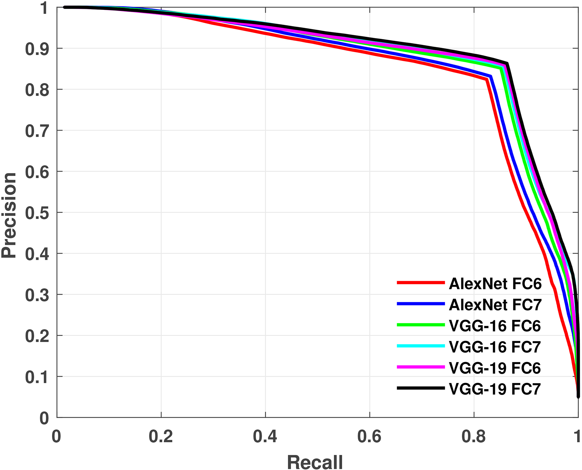

Figure 5.

MAP values using different number of DCT coefficients on both datasets.

Figure 6.

MAP as a function of different PCA components.

Normally, the number of deep features is relatively high, and when using similarity measures, the matching process becomes very slow; therefore, reducing the number of features will enhance the searching speed for query images. It is important in this case to reduce the number of features without affecting the CBIR system accuracy. Reduction techniques such as DCT, PCA or DWT significantly reduce the dimensionality of the feature vectors, while maintaining effective system performance.

Based on Table 8(c), we selected the first N coefficients to approximate the original signal to a smaller number of coefficients. Figure 5 illustrates the effect of the number of DCT coefficients used on the CBIR system MAP.

Intuitively, using more DCT coefficients results in a higher MAP being obtained; however, a closer look at Fig. 5 reveals that the MAP becomes extremely close to that of the original signal when using only 300 coefficients on both datasets, which allows for faster CBIR without affecting the retrieving results. PCA reduces the dimensionality more effectively than DCT, by obtaining almost the same results with a significantly lower number of features. For example, Table 8(d) illustrates the MAP using only 10 principal components (those with the highest data variance) with different distance metrics, while Table 8(e) illustrates the CBIR MAP using the same number of components after normalising the data.

Table 9

MAP and number of features for each DWT level

Level	Number of features	MAP of Corel-1000	MAP of Coil-20
Without DWT	4096	0.842	0.901
1	2048	0.80	0.894
2	1024	0.734	0.879
3	512	0.662	0.848

Figure 7.

ER of all deep features following each retrieved image.

As can be seen from Table 8(d) and 8(e), the MAP is still high after transforming the features from 4096 to 10-dimensions. In this case, ED and MD perform better, owing to the small number of features, which reduces the probability of features that dominate the distance.

We opted to use the 10 components of PCA for the experiments displayed in Table 8(e), because using these achieves the highest system MAP, as indicated in Fig. 6. Despite the fact that there are several methods to determine the number of components to be used for PCA [31, 5], in this study, we wish to show that choosing the right number of components is critical for CBIR systems as it can be seen in Fig. 6.

Table 10

MAP and ER of different deep features compared to the low-level features presented in [9] on the Corel-1000 dataset

Features	MAP	ER
Colour histogram	0.505	0.169
LF SIFT global search	0.383	0.372
LF patches histogram	0.483	0.179
LF SIFT histogram	0.482	0.256
Inv. feature histogram (monomial)	0.476	0.192
MPEG7: scalable color	0.467	0.251
LF patches signature	0.404	0.243
Gabor histogram	0.413	0.305
32 x 32 image	0.376	0.472
MPEG7: color layout	0.418	0.354
X x 32 image	0.243	0.559
Tamura texture histogram	0.382	0.284
LF SIFT signature	0.367	0.351
Grey value histogram	0.317	0.453
LF patches global	0.305	0.429
MPEG7: edge histogram	0.408	0.328
Inv. feature histogram (relational)	0.349	0.383
Gabor vector	0.237	0.655
Global texture feature	0.263	0.514
AlexNet FC6	0.786	0.044
AlexNet FC7	0.801	0.043
VGG-16 FC6	0.862	0.032
VGG-16 FC7	0.872	0.026
VGG-19 FC6	0.864	0.026
VGG-19 FC7	0.873	0.028

In order to investigate the effect of the dimensionality reduction of the deep features on the CBIR system MAP further, we used the DWT for dimensionality reduction, as in [1, 63]. We applied three decomposition levels, and at each DWT level, the number of features was reduced by half. Table 9 illustrates the system performance after three decomposition levels using the VGG-16 FC6 and VGG-19 FC6 with CD (with the best features and distance metric indicated in Table 8(a)) on both datasets.

As can be observed from Table 9, the signal or feature vector began to change as the number of levels used increased, as the MAP deceased by approximately 7% after each level on the Corel-1000 dataset, which is a significant system performance degradation. In the case of the Coil-20 dataset, the loss was not significant; however, the CBIR system performance with dimensionality reduction using DWT was not satisfactory if compared to DCT and PCA, in terms of the number of features and system MAP. Converting the features into PDF reduces the dimensionality by grouping the features in the same range in order to produce less length feature vectors [23]. Table 8(f) presents the MAP of the 10 bins PDF using the studied distances.

It can be noted from Table 8(f) that the results are not satisfactory. Perhaps grouping the same range deep features together in a bin reduces the significance of the features by being in their original place. Moreover, binning does not transform the features in a specific manner within a space, but simply performs blind grouping without prior information regarding the features, while it may be effective for special features as in [23], it appears not to with complex structure features such as deep features. The term error rate (ER) is used as an evaluation measure in this comparison, and is given by $1-p(1)$ , where $p(1)$ is the precision at the first retrieved image. In general, a lower error rate means that the relevant images are retrieved earlier. Table 10 displays the best MAP and ER values for different deep features (all deep features using CD with DCT and normalisation, as in Table 8(c)) compared to the low-level features presented in [9].

Figure 7 presents the ER following each retrieved image up to 99, which is the number of relevant images of each image in the Corel-1000 dataset.

As can be seen from Fig. 7, very deep features such as VGG-19 FC7 yield a lower ER than less deep features such AlexNet FC6. In VGG models, the relevant images are retrieved earlier than in the AlexNet feature.

8. Conclusion

In this paper, different types of low-level and deep features for CBIR have been tested and compared. The comparison was conducted using different SR and CL methods, and various similarity measures with different validation approaches. Furthermore, we examined the features with/without data normalization and experimentally demonstrated the effect of different dimensionality reduction techniques on the system performance, using two popular data sets in this field.

Eight hundred forty-two different tests are done on both Corel and Coil datasets using different SR methods, dictionary learning algorithms, similarity measures, dimensional reduction techniques and many deep features from different layers deep models.

Results show that combination of DL and SR lead to accurate retrieval models. Especially, when the results of these combinations are compared with LFD based SR, the usage of DL as deep features increase the retrieval accuracy.

The experimental results indicate high MAPs on both datasets using $K$ -SVD and homotopy, particularly when using a small dictionary size. However, in general, SSF achieved the best results, while the VGG-16 features were optimum in the SR framework. Despite the fact that SSF is rarely used in CBIR systems, in this study, it is proven that the SSF overcomes the other common CL algorithms. Therefore testing SSF with different surrogate functions is recommended for future studies.

We determined that the system performance varies based on the used distance and pre-processing methods. In general, the VGG models performed better in extracting more efficient features.

Selecting the optimal distance relies on the data itself, and in this study, CD and HD achieved superior performance to MD and ED in most cases. However, in the case of PCA reduction, ED provided superior results to the other metrics. Furthermore, the results indicate that the deep features can be enhanced by using DCT as a pre-processing stage. Such a step increases the system performance and achieves higher accuracy than using the pure deep features; however, selecting the appropriate distance metric is critical to the system performance following pre-processing.

Moreover, PCA was found to be the most suitable option among the investigated dimensionality reduction algorithms, as it reduced the dimensionality of the deep features dramatically, to 10 features, while maintaining effective performance. Similarly, the DCT provides a high approximation of the performance with the original features, by using only 300 features.

In future studies, we will investigate the performance of SSF with deep features in many other computer vision problems, including face recognition, fingerprint identification and authentication, facial and medical image retrieval, etc. Studying the response time of the discussed SR methods with the deep features is also planned. Moreover, we are going to conduct some experiments for comparison among state-of-the-art approaches to study how they work with the high-level and low-level features over different approaches and show the effectiveness. For instance, [28] proposed various masking schemes to select a representative subset of local convolutional features and employed recent embedding and aggregating methods to further enhance feature discriminability. In addition to the high-level and low-level features, there are more features to be extracted, such as those extracted from halftoning-based block truncation coding. For instance, [17] proposed color co-occurrence feature (CCF) and bit pattern features (BPF) extracted from block truncation coding to exploit the advantage of efficient ordered-dither block truncation coding for image content descriptor generation. Such features will be investigated in our future work, along with conducting more feature selection experiments to observe what features are indeed crucial. We also plan to increase the speed of the retrieval process using efficient indexing techniques, such as, [45, 26, 20, 21].

Footnotes

Acknowledgments

The first author would like to thank Tempus Public Foundation for sponsoring his PhD study, also, this paper is under the project EFOP-3.6.3-VEKOP-16-2017-00001 (Talent Management in Autonomous Vehicle Control Technologies), and supported by the Hungarian Government and co-financed by the European Social Fund.

References

Agarwal

Verma

and Dixit

, Content based image retrieval using color edge detection and discrete wavelet transform, In Issues and Challenges in Intelligent Computing Techniques (ICICT), 2014 International Conference on, IEEE, 2014, pp. 368–372.

Aggarwal

C.C.

Hinneburg

and Keim

D.A.

, On the surprising behavior of distance metrics in high dimensional space, In International conference on database theory, Springer, 2001, pp. 420–434.

Ashraf

Ahmed

Jabbar

Khalid

Ahmad

Din

and Jeon

, Content based image retrieval by using color descriptor and discrete wavelet transform, Journal of Medical Systems 42(3) (2018), 44.

Bay

Ess

Tuytelaars

and Van Gool

, Speeded-up robust features (surf), Computer vision and Image Understanding 110(3) (2008), 346–359.

Cangelosi

and Goriely

, Component retention in principal component analysis with application to cdna microarray data, Biology Direct 2(1) (2007), 2.

Celik

and Bilge

H.S.

, Content based image retrieval with sparse representations and local feature descriptors: A comparative study, Pattern Recognition ]68 (2017), 1–13.

Cheng

Zhou

and Han

, Learning rotation-invariant convolutional neural networks for object detection in vhr optical remote sensing images, IEEE Transactions on Geoscience and Remote Sensing 54(12) (2016), 7405–7415.

Desai

and Sonawane

, Gist, hog and dwt-based content-based image retrieval for facial images, In Proceedings of the International Conference on Data Engineering and Communication Technology, Springer, 2017, pp. 297–307.

Deselaers

Keysers

and Ney

, Features for image retrieval: an experimental comparison, Information Retrieval 11(2) (2008), 77–107.

10.

Dong

Loy

C.C.

and Tang

, Image super-resolution using deep convolutional networks, IEEE Transactions on Pattern Analysis and Machine Intelligence 38(2) (2016), 295–307.

11.

ElAlami

M.E.

, A new matching strategy for content based image retrieval system, Applied Soft Computing 14 (2014), 407–418.

12.

Emran

S.M.

and Ye

, Robustness of canberra metric in computer intrusion detection, In Proc. IEEE Workshop on Information Assurance and Security, West Point, NY, USA, 2001.

13.

Folkers

and Samet

, Content-based image retrieval using fourier descriptors on a logo database, In Pattern Recognition, 2002. Proceedings. 16th International Conference on, volume 3, IEEE, 2002, pp. 521–524.

14.

Gao

Zhang

Jia

and Zhang

, Single sample face recognition via learning deep supervised autoencoders, IEEE Transactions on Information Forensics and Security 10(10) (2015), 2108–2118.

15.

Ghosh

and Chellappa

, Deep feature extraction in the dct domain, In Pattern Recognition (ICPR), 2016 23rd International Conference on, IEEE, 2016, pp. 3536–3541.

16.

Goh

Thome

Cord

and Lim

J.-H.

, Learning deep hierarchical visual feature coding, IEEE Transactions on Neural Networks and Learning Systems, 25(12) (2014), 2212–2225.

17.

Guo

J.-M.

and Prasetyo

, Content-based image retrieval using features extracted from halftoning-based block truncation coding, IEEE Transactions on Image Processing 24(3) (2015), 1010–1024.

18.

Gupta

and Garg

A.K.

, Analysis of image compression algorithm using dct, International Journal of Engineering Research and Applications (IJERA) 2(1) (2012), 515–521.

19.

Hassanat

, Visual speech recognition, arXiv preprint arXiv:1409.1411, 2014.

20.

Hassanat

, Furthest-pair-based decision trees: Experimental results on big data classification, Information 9(11) (2018), 284.

21.

Hassanat

, Norm-based binary search trees for speeding up knn big data classification, Computers 7(4) (2018), 54.

22.

Hassanat

Btoush

Abbadi

M.A.

Al-Mahadeen

B.M.

Al-Awadi

Mseidein

K.I.

Almseden

A.M.

Tarawneh

A.S.

Alhasanat

M.B.

Prasath

V.S.

et al., Victory sign biometrie for terrorists identification: Preliminary results, In Information and Communication Systems (ICICS), 2017 8th International Conference on, IEEE, 2017, pp. 182–187.

23.

Hassanat

Prasathb

Al-kasassbeh

Tarawneh

A.S.

and Al-shamailh

A.J.

, Magnetic energy-based feature extraction for low-quality fingerprint images, Signal, Image and Video Processing May 2018, doi: 10.1007/s11760-018-1302-0:1-8.

24.

Hassanat

and Tarawneh

A.S.

, fusion of color and statistc features for enhancing content-based image retrieval systems, Journal of Theoretical & Applied Information Technology 88(3) (2016).

25.

Hassanat

A.B.

, Dimensionality invariant similarity measure, Journal of American Science 10(8) (2014), 221–226.

26.

Hassanat

A.B.

, Furthest-pair-based binary search tree for speeding big data classification using k-nearest neighbors, Big Data 6(3) (2018), 225–235.

27.

Hassanat

A.B.

Prasath

V.S.

Al-Mahadeen

B.M.

and Alhasanat

S.M.M.

, Classification and gender recognition from veiled-faces, International Journal of Biometrics 9(4) (2017), 347–364.

28.

Hoang

T.-T.

Le Tan

D.-K.

and Cheung

N.-M.

, Selective deep convolutional features for image retrieval, In Proceedings of the 25th ACM international conference on Multimedia, ACM, 2017, pp. 1600–1608.

29.

Hossen

M.K.

and Tuli

S.H.

, A surveillance system based on motion detection and motion estimation using optical flow, In Informatics, Electronics and Vision (ICIEV), 2016 5th International Conference on, IEEE, 2016, pp. 646–651.

30.

Hsu

Lee

M.L.

and Zhang

, Image mining: Trends and developments, Journal of Intelligent Information Systems 19(1) (2002), 7–23.

31.

Jackson

D.A.

, Stopping rules in principal components analysis: a comparison of heuristical and statistical approaches, Ecology 74(8) (1993), 2204–2214.

32.

Jhanwar

Chaudhuri

Seetharaman

and Zavidovique

, Content based image retrieval using motif cooccurrence matrix. Image and Vision Computing 22(14) (2004), 1211–1220.

33.

Kappeler

Yoo

Dai

and Katsaggelos

A.K.

, Video super-resolution with convolutional neural networks, IEEE Transactions on Computational Imaging 2(2) (2016), 109–122.

34.

Khatami

Babaie

Tizhoosh

Khosravi

Nguyen

and Nahavandi

, A sequential search-space shrinking using cnn transfer learning and a radon projection pool for medical image retrieval, Expert Systems with Applications 100 (2018), 224–233.

35.

Krizhevsky

Sutskever

and Hinton

G.E.

, Imagenet classification with deep convolutional neural networks, In Advances in neural information processing systems, 2012, pp. 1097–1105.

36.

Kyrki

Kamarainen

J.-K.

and Kälviäinen

, Simple gabor feature space for invariant object recognition, Pattern Recognition Letters 25(3) (2004), 311–318.

37.

Lance

G.N.

and Williams

W.T.

, Mixed-data classificatory programs i – agglomerative systems, Australian Computer Journal 1(1) (1967), 15–20.

38.

Lande

M.V.

Bhanodiya

and Jain

, An effective content-based image retrieval using color, texture and shape feature, In Intelligent Computing, Networking and Informatics, Springer, 2014, pp. 1163–1170.

39.

Lei

Mei

Zheng

Dong

Zhou

and Fan

, Learning group-based dictionaries for discriminative image representation, Pattern Recognition 47(2) (2014), 899–913.

40.

Lei

and Li

S.Z.

, Learning stacked image descriptor for face recognition, IEEE Transactions on Circuits and Systems for Video Technology 26(9) (2016), 1685–1696.

41.

Lee

M.-C.

and Pun

C.-M.

, Complex zernike moments features for shape-based image retrieval, IEEE Transactions on Systems, Man and Cybernetics-Part A: Systems and Humans 39(1) (2009), 227–237.

42.

Liu

Wang

Wen

Yang

Han

and Huang

T.S.

, Robust single image super-resolution via deep networks with sparse prior, IEEE Transactions on Image Processing 25(7) (2016), 3194–3207.

43.

Lowe

, Distinctive image features from scale-invariant keypoints, International Journal of Computer Vision 60(2) (2004), 91–110.

44.

Lowe

D.G.

, Distinctive image features from scale-invariant keypoints, International Journal of Computer Vision 60(2) (2004), 91–110.

45.

Novak

Batko

and Zezula

, Large-scale image retrieval using neural net descriptors, In Proceedings of the 38th international ACM SIGIR conference on research and development in information retrieval, ACM, 2015, pp. 1039–1040.

46.

Pang

Orgun

M.A.

and Yu

, A novel biomedical image indexing and retrieval system via deep preference learning, Computer Methods and Programs in Biomedicine 158 (2018), 53–69.

47.

Pang

Yuan

and Pan

, Efficient hog human detection, Signal Processing 91(4) (2011), 773–781.

48.

Park

Jin

J.S.

and Wilson

L.S.

, Fast content-based image retrieval using quasi-gabor filter and reduction of image feature dimension, In Image Analysis and Interpretation, 2002. Proceedings. Fifth IEEE Southwest Symposium on, IEEE, 2002, pp. 178–182.

49.

Prasath

Alfeilat

H.A.A.

Lasassmeh

and Hassanat

, Distance and similarity measures effect on the performance of k-nearest neighbor classifier-a review, arXiv preprint arXiv:1708.04321, 2017.

50.

Quellec

Charrière

Boudi

Cochener

and Lamard

, Deep image mining for diabetic retinopathy screening, Medical Image Analysis 39 (2017), 178–193.

51.

Ramasamy

Athisayam

J.S.K.

and Thangaraj

, An edge directed gabor features for efficient image retrieval, Advances in Natural and Applied Sciences 11(3) (2017), 6–24.

52.

Rashedi

Nezamabadi-Pour

and Saryazdi

, A simultaneous feature adaptation and feature selection method for content-based image retrieval systems, Knowledge-Based Systems 39 (2013), 85–94.

53.

Reich

Price

A.L.

and Patterson

, Principal component analysis of genetic data, Nature Genetics 40(5) (2008), 491.

54.

Romero

Gatta

and Camps-Valls

, Unsupervised deep feature extraction for remote sensing image classification, IEEE Transactions on Geoscience and Remote Sensing 54(3) (2016), 1349–1362.

55.

Sanu

S.G.

and Tamase

P.S.

, Satellite image mining using content based image retrieval, International Journal of Engineering Science (2017), 13928.

56.

Saritha

R.R.

Paul

and Kumar

P.G.

, Content based image retrieval using deep learning process, Cluster Computing (2018), 1–14.

57.

Simonyan

and Zisserman

, Very deep convolutional networks for large-scale image recognition, arXiv preprint arXiv:1409.1556, 2014.

58.

Smeulders

A.W.

Worring

Santini

Gupta

and Jain

, Content-based image retrieval at the end of the early years, IEEE Transactions on Pattern Analysis and Machine Intelligence 22(12) (2000), 1349–1380.

59.

Squire

D.M.

Müller

and Pun

, Content-based query of image databases: inspirations from text retrieval, Pattern Recognition Letters 21(13-14) (2000), 1193–1198.

60.

Srivastava

and Khare

, Content-based image retrieval using local binary curvelet co-occurrence pattern – a multiresolution technique, The Computer Journal (2017), 1–17.

61.

Subrahmanyam

Q.J.

Maheshwari

and Balasubramanian

, Modified color motif co-occurrence matrix for image indexing and retrieval, Computers & Electrical Engineering 39(3) (2013), 762–774.

62.

Tarawneh

Chetverikov

and Hassanat

, Pilot comparative study of different deep features for palmprint identification in low-quality images, In Ninth Hungarian Conference on Computer Graphics and Geometry, Hungary-Budapest, Mar 2018.

63.

Tarawneh

A.S.

Chetverikov

Verma

and Hassanat

A.B.

, Stability and reduction of statistical features for image classification and retrieval: Preliminary results, In 2018 9th International Conference on Information and Communication Systems (ICICS), April 2018, pp. 117–121.

64.

Tzelepi

and Tefas

, Deep convolutional learning for content based image retrieval, Neurocomputing 275 (2018), 2467–2478.

65.

Varish

and Pal

A.K.

, A novel image retrieval scheme using gray level co-occurrence matrix descriptors of discrete cosine transform based residual image, Applied Intelligence (2018), 1–24.

66.

Wang

X.-Y.

Y.-J.

and Yang

H.-Y.

, An effective image retrieval scheme using color, texture and shape features, Computer Standards & Interfaces 33(1) (2011), 59–68.

67.

Wells

W.M.

, III., Medical image analysis – past, present and future, 2016.

68.

Xia

Wang

Zhang

Qin

Sun

and Ren

, A privacy-preserving and copy-deterrence content-based image retrieval scheme in cloud computing, IEEE Transactions on Information Forensics and Security 11(11) (2016), 2594–2608.

69.

Zhang

Wong

Indrawan

and Lu

, Content-based image retrieval using gabor texture features, IEEE Transactions PAMI (2000), 13–15.

70.

Zhang

Yang

L.T.

Chen

and Li

, A survey on deep learning for big data, Information Fusion 42 (2018), 146–157.

71.

Zhang

Yao

Sun

and Lu

, Sparse coding based visual tracking: Review and experimental comparison, Pattern Recognition 46(7) (2013), 1772–1788.

72.

Zhao

and Wang

, Heterogeneous feature selection with multi-modal deep neural networks and sparse group lasso, IEEE Transactions on Multimedia 17(11) (2015), 1936–1948.

73.

Zhou

J.-X.

Liu

X.-D.

T.-W.

Gan

J.-H.

and Liu

W.-Q.

, A new fusion approach for content based image retrieval with color histogram and local directional pattern, International Journal of Machine Learning and Cybernetics 9(4) (2018), 677–689.

74.

Zhu

Yeh

M.-C.

Cheng

K.-T.

and Avidan

, Fast human detection using a cascade of histograms of oriented gradients, In Computer Vision and Pattern Recognition, 2006 IEEE Computer Society Conference on, volume 2, IEEE, 2006, pp. 1491–1498.

75.

Zibulevsky

and Elad

, L1-l2 optimization in signal and image processing, IEEE Signal Processing Magazine 27(3) (2010), 76–88.

512-D $K$ -means
	Low-level features					Deep features
CL algorithms	SIFT	SURF	HOG	LBP	LTP	AlexNet FC6	AlexNet FC7	VGG-16 FC6	VGG-16 FC7	VGG-19 FC6	VGG-19 FC7
Homotopy	0.43	0.40	0.52	0.57	0.5	0.15	0.16	0.16	0.18	0.16	0.15
Lasso	0.43	0.37	0.50	0.47	0.38	0.16	0.16	0.17	0.16	0.18	0.15
Elastic net	0.43	0.32	0.49	0.20	0.37	0.14	0.15	0.14	0.14	0.15	0.15
SSF	0.50	0.39	0.44	0.54	0.53	0.44	0.49	0.47	0.50	0.48	0.51

Detailed investigation of deep features with sparse representation and dimensionality reduction in CBIR: A comparative study

Abstract

Keywords

1. Introduction

3. Materials and methods

3.1 Low-level features

3.1.1 Gabor features

3.1.3 SIFT and SURF

3.2 High-level features

4. Dimensionality reduction

4.1 DCT

4.3 DWT

5.1 Euclidian distance

Table 6 Average MAP values of all CL used for all dictionary sizes

Footnotes

Acknowledgments

References

Table 6
Average MAP values of all CL used for all dictionary sizes