
Abstract
In this paper, we present a method for exploratory data analysis of streaming data based on probabilistic graphical models (latent variable models). This method is illustrated by concept drift tracking, using financial client data from a European regional bank. For this particular setting, the analyzed data spans the period from April 2007 to March 2014 and therefore starts before the beginning of the financial crisis of 2008. The implied changes in the economic climate during this period manifests itself as concept drift in the underlying data generating distribution. We explore and analyze this financial client data using a probabilistic graphical modeling framework that provides an explicit representation of concept drift as an integral part of the model. We show how learning these types of models from data provides additional insight into the hidden mechanisms governing the drift in the domain. We present an iterative approach for identifying disparate factors that jointly account for the drift in the domain. This includes a semantic characterization of one of the main influencing drift factors. Based on the experiences and results obtained from analyzing the financial data, we discuss the applicability of the framework within a more general context.
Introduction
Performing data analysis in a streaming context raises several important issues that are often less pronounced when conducting batch data analysis. In particular, the instances in a data stream can often not be assumed independent, and when the data stream exhibits concept drift the underlying data generating distribution may change over time [10]. If the concept drift inherent in the domain is not carefully taken into account, the result can be a deterioration of accuracy when doing classification or, more generally, failure to capture and interpret intrinsic properties of the data during data exploration.
In collaboration with a European regional bank (Banco de Crédito Cooperativo, BCC), we have been conducting data analysis over a subset of their clients based on client-specific financial information captured during the period from April 2007 to March 2014. Specifically, the focus has been on real-time analysis, detection, and interpretation of financial changes during this period. Particular attention has been given to two groups of clients, defined by whether or not they will default on their financial obligations within the following 12 months.
The period during which data has been collected starts before the beginning of the financial crisis, hence the general economic climate exhibits changes during the collection period. This is also directly reflected in the client data, where we, for instance, see the drifts in the average monthly account balances as illustrated in Fig. 1d. Note that the drift is more pronounced for the defaulting clients than for the non-defaulting clients and that we also see a slightly inverse trend for the two client groups. This is the reason why we included defaulting information in the analysis. Another example of drift can be seen for the unpaid amount in mortgages for the two groups as shown in Fig. 1e.
Mean evolution of all predictive variables for defaulting and non-defaulting clients (monthly aggregated). The ranges on the y-axes, both here and in successive figures, have been deliberately removed for confidentiality reasons.
Generally, when comparing these two financial indicators, we see that they exhibit different types of concept drift, and that a common/global contextual cause is not immediately apparent from the data. We would like, therefore, to go beyond this immediate analysis and instead consider ‘broader’ types of concept drift that are less variable-specific and which influence and govern several key financial indicators simultaneously and across client groups. We thus adopt the general definition of concept drift from [10], where concept drift is defined as the existence of two consecutive time points for which the joint distribution over the domain variables differ. Since this definition does not rely on a designated target variable, we can position the problem as unsupervised concept drift detection and analysis [19].
In this paper, we further explore and extend a recently proposed model for capturing concept drift [3]. The model proposed by [3] is based on probabilistic graphical models and provides a principled approach for capturing concept drift by letting the drift be encoded explicitly within the model class. There are several advantages to this approach. First of all, the model does not rely on any of the standard techniques to deal with concept drift, see [10] and the references therein. Such techniques, including external concept drift detectors that, e.g., would use changes in classification accuracy to imply a form of supervised concept drift, often require information that only becomes available after a certain time delay [9, 24] (such as the true class labels). Secondly, by letting concept drift be an explicit and integral part of the modeling framework, we have added support for semantic interpretations of potential drifts. In particular, concept drift can immediately be linked to selected model components enabling an analysis of how concept drift affects different parts of the model. The proposed method therefore not only provides an unsupervised way of detecting concept drift, but it may also enable a more systematic analysis of the (local) domain-specific factors that drive concept drift; this type of insight is not immediately provided when, e.g., involving external concept drift detectors.
In comparison with the analysis conducted in [3], the contributions of the present paper includes an extension of the model class of [3] that enables a more fine-grained concept drift analysis targeting individual variables. Furthermore, we propose an iterative approach for identifying disparate factors that jointly account for the drifts in the domain. We demonstrate the use of the proposed methods based on the financial data set supplied by BCC. The results of the analysis include the identification and semantic characterization of one of the key factors governing concept drift for this particular domain. Lastly, we discuss the proposed modeling framework in a more general setting, linking model validation and concept drift analysis. The proposed methods are released as part of an open-source toolbox for scalable probabilistic machine learning (
The remainder of the paper is organized as follows. In Section 2 we give an overview of other related works. In Section 3 we provide a detailed description and analysis of the data set that is used in the study. Section 4 discusses and analyzes the modeling framework introduced by [3], on which the concept drift analysis presented in Section 5 is based. In Section 6 we position our analysis within a more general context, providing a critical discussion of the limitations of our procedure as well as possible extensions to the framework and open research questions. Lastly, we give some concluding remarks in Section 7.
The topic of concept drift is referred to in the literature under different terms (e.g., population drift, concept shift), and sometimes they relate to similar problems but with different nuances. It can refer to a change in the probability distributions of some observed variables, or of some latent parameter or hyperparameter, or even to a change in the problem itself (for instance, when there is a redefinition of the class labels in a classification problem). Several different approaches have been studied in recent years. We make a brief revision of some of them.
In [14], the authors analyze the problem of making predictions in the future when there is a change in the population distributions, from the point of view of the classification performance. To do so, a time series model (linear or generalized linear model) is proposed. In [7], the authors tackle a similar problem. They try to detect changes in the probability distribution over the test set, as compared to the validation set, finding what they call fracture points. Their technique is based on detecting bias using statistical tests, and they evaluate it using various datasets. Another related study is [11], in which the problem of detecting the deterioration of a classifier’s performance is addressed. This method assumes that the class distribution changes from a time point to another, but the conditional distributions remain the same. The approach is tested on a credit scoring real-world dataset.
The work in [6] focuses on the financial domain, especially in the probability of default. The authors use hypothesis tests to determine if there has been a drift in the predictive accuracy. The final decision is based on the
In [16], the authors propose a technique for detecting shifts in churn models using an information-theory metric called stability index, closely related to the Kullback-Leibler divergence. The decision on the presence of shifts is based on this metric and a threshold. Finally, [20] is a thorough review of the literature of concept drift and related problems. In it, the authors try to provide unifying definitions and concepts, and to clarify the different approaches that have been proposed.
Several of these attempts [6, 7] rely on statistical tests to decide whether there are significant differences between the expected and the actual performance of the model when making predictions. This can be problematic for large datasets, in a streaming context or if any underlying assumption fails. In some other approaches [6, 14, 16], the proposed methodology is able to give some alert when there are significant drifts in the model (often called backtesting), but the model is not updated accordingly.
The approach that we propose in this paper does not rely on the presence of class labels, as all the previous methods do, and it is able to detect different kinds of changes in the data distribution, or concept drifts. Moreover, it deals naturally with streaming data and allows to update the model immediately when new data are available.
Description of the data
The data set, provided by BCC, contains monthly aggregated information for a set of BCC clients for the period from April 2007 to March 2014. Only “active” clients are considered, meaning that we restrict our attention to individuals between 18 and 65 years of age, who have at least one automatic bill payment or direct debit in their accounts. To make the data set as homogeneous as possible, we only retain clients residing in the region of Almería (a mainly agricultural area in the south of Spain), and excluded BCC employees, since they have special banking conditions. We reduced the resulting data set so that it only includes 50 000 clients each month.
Up until December 2010 there are some clients that only become active every six months (due to periodic fees). From December 2010 and until the end of the period this pattern appears every 3 months [3]. The particular clients involved vary, and removing them from the overall data set is therefore not feasible. Instead, and in order to avoid the seasonal peaks produced by these known patterns, we remove the affected 21 months.1
The analysis of the experiments in this paper are practically the same if we consider the peak months, except that the results are noisier around these months [3].
Assisted by BCC’s experts, we extracted six variables from the resulting data set that encode monthly aggregated information, and which collectively describe the financial status of a client. Figure 1 shows the evolution of these variables for both defaulting and non-defaulting clients throughout the period. We note that some clients may have missing values for some of the variables for a given month (e.g., because a client was not active during that particular month). However, the generative nature of the models we employ (detailed in the following section) ensures that these missing values are naturally handled within the model and do not need to be treated separately. Finally, each client also has an associated class variable, which indicates if that particular client will default during the following 12 months.
If we take a closer look at the attributes, we observe several characteristics that could further challenge the modeling process. Figure 2 shows the histograms for a couple of variables. The first thing we notice is the high density of zeros, but also the long-tails of the distributions. The latter results in large variances for most of the attributes.
Histograms for two of the predictive attributes. Ranges in the x-axes have been deliberately removed for confidentiality reasons.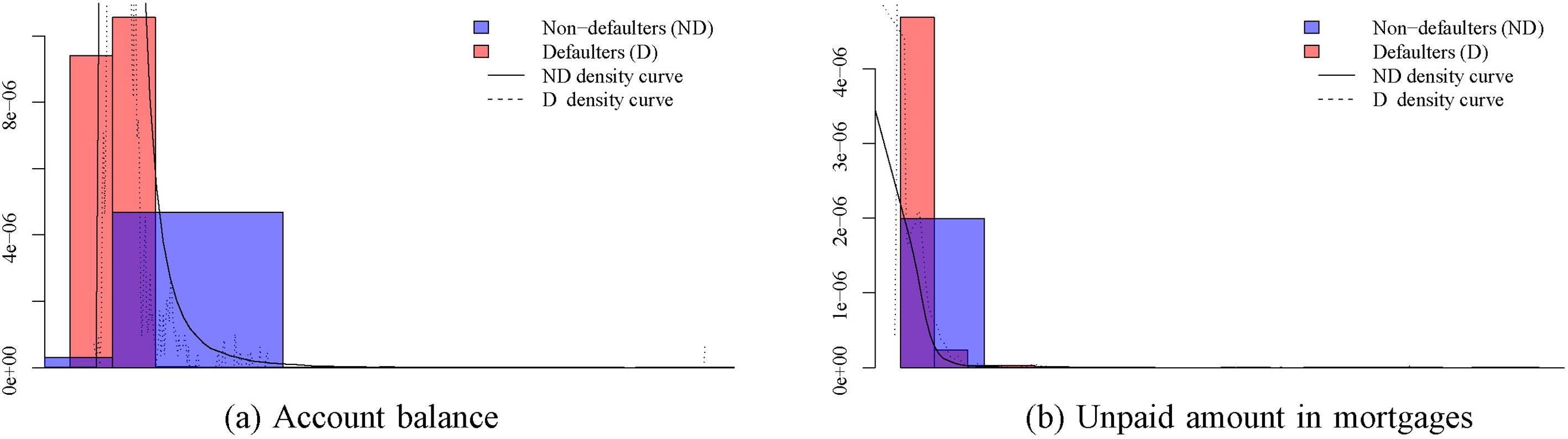
When also considering the evolution of the means in Fig. 1 we can see at least two tendencies in the data. One general trend of gradual and monotonic movement and the other of seasonal changes usually peaking at the end of the year. Thus, the data sets appear to exhibit different types of concept drift.
The drift in the data indicates the need for a model that takes these changes into account. More specifically, we are interested in a simple density estimator that is able to detect the different tendencies over multiple attributes simultaneously while also maintaining the defaulting/non-defaulting distinction of the clients. The following section introduces and discusses the particular model type we have used for the analysis.
Concept drift detection and adaptation have typically been considered within a supervised learning context, where changes in model accuracy are seen as an indication of concept drift [10]. This means that concept drift detection is closely linked to a specific prediction task, which may be too restrictive for an exploratory data analysis setting. For example, labeled streaming data is needed in order to evaluate changes in classification accuracy, but these labels often come with a (significant) time delay. For example, for our financial setting described in Section 3, if the future defaulting status of a client is considered as the class variable, then the true class label will only be revealed after a delay of twelve months.
Instead we consider the framework for detecting and analyzing concept drift presented by [3], in which the key idea is to explicitly represent concept drift as an integral part of the model definition without relying on a designated target variable. Thus, the framework considers concept drift as the existence of an instance
The modeling framework proposed by [3] is illustrated using plate notation in Fig. 3 and can be seen as a special type of probabilistic graphical model [15]. In the figure,
We explicitly represent the class variable in this context as it is a requirement of the BCC experts to have a clear distinction between defaulter and non-defaulter clients. Since the percentage of defaulter clients is small, this ensures that this group of clients is modeled separately. We stress again, however, that our general concept drift model is not relying on classification accuracy to detect concept drift.
Model of concept drift [3]. In this model structure it is assumed that 
The overall framework is positioned in the Bayesian paradigm, where both parameters and unobserved variables (
Bayesian inference is in general NP-hard [8] and for the type of hybrid dynamic models considered in this paper (detailed in the following section) exact inference is intractable. Thus, we resort to approximate inference/learning based on a variational Bayes inference engine [13, 1]. Variational Bayes can be seen as a gradient ascent algorithm, and when constraining the (conditional) distributions to be members of the conjugate exponential family, it can be implemented through variational message passing (VMP) [23].
There are several benefits of this approach, including i) having concept drift as an integral part of a holistic model; ii) concept drift is explicitly represented and therefore open for investigation; iii) immediate model validation; iv) good fit in terms of marginal log-likelihood to complex data, even for this rather parsimonious model.
A proof of concept of this modeling framework can be found in Appendix B, where we analyze two synthetic data sets widely employed as benchmarks in the concept drift literature. This analysis verifies the applicability of this framework for modeling concept drift beyond the financial domain, which is the focus of this work.
In this section, we detail the instantiation of the general methodology presented in Section 4 with respect to our financial data set in order to analyze the trend in the evolution of the financial profile of the clients. For this, we use a publicly available toolbox,3
The code and models used in this paper can be downloaded from the AMIDST Toolbox webpage (through its GitHub repository):
We consider two general types of models. First, we explore a model containing a hidden variable
As a first step we employ a variant of the models presented in Section 4 to track concept drift of individual attributes. In this way, we examine whether or not the six attributes in our data set exhibit different drift behavior. This simpler setting also allows us to better illustrate how our approach captures the general trend in the data over time.
We make a simple instantiation of the general framework, where each attribute is linearly dependent on a local hidden variable, which enables the use of efficient learning algorithms. More complex (non-linear) dependencies could eventually be used by employing alternative parametrizations of the conditional probability distributions, at the cost of having to use more complex learning algorithms.
More precisely, we use a concept drift model with a hidden variable
where
Using standard properties of the Gaussian distribution, we then have that
In Fig. 4 we plot a detailed result of this analysis for two attributes: Account Balance (AB) and Unpaid Amount in Mortgages (UM), respectively. All means in the normal distributions have been arbitrarily initialized to zero:
Two series defined by
Considering Fig. 4 we can make the following tentative conclusions:
The series The The movements of the time series are scaled by the values of their Due to confidentiality reasons, we are unfortunately not able to disclose the
Empirical, model means, and the expectation of the local hidden variables for the two feature variables Att4 and Att5. More specifically, 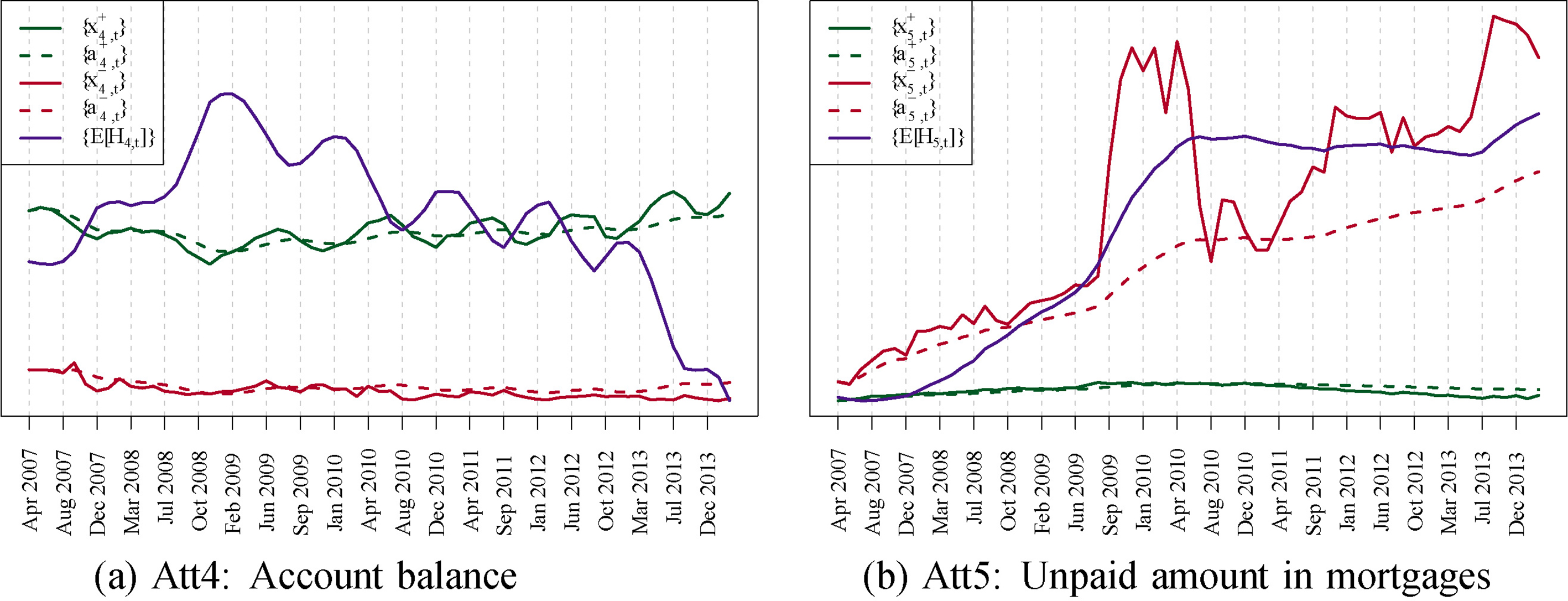
Finally, in Fig. 10 we plot the set of
It is interesting to see in Fig. 10 how we can clearly identify two groups of attributes with different evolution trends. On the one hand, we have that the attributes “Total Credit Amount”, “Unpaid Amount in Mortgages” and “Unpaid Amount in Personal Loans” (Att1, Att5 and Att6 respectively) exhibit a kind of monotonically increasing trend over time, with no seasonality. According to our BCC’s experts, they mainly show the financial deterioration of the defaulting clients (c.f. Fig. 1): higher unpaid amount in mortgages and higher total credit loans, although for “Unpaid Amount in Personal Loans” we can see a slow reduction across the period. The latter is because personal loans are typically small short term loans with high-interest rates, which clients prefer to pay back on time. Another effect comes into play here: during the observation period, many weak non-defaulter clients changed to the group of defaulting clients, leaving in the former group those clients that were more robust to changes in the economic climate. This translates into an improvement of the financial profile of the group of non-defaulter clients.
The other group of attributes, “Income”, “Expenses” and “Account Balance” (Att2, Att3 and Att4 respectively), identified in Fig. 10, presents a yearly seasonal pattern down-peaking at the end of the year, which characterizes the particular financial profile of the BCC’s clients. The “Account Balance” attribute seems to have a more complex evolution, which will be discussed in more detail in the next section.
During the analysis above we have deliberately neglected that the estimators
In the previous section, we looked at the individual trends of each of the attributes. In this section, we are interested in capturing the joint global trend of all of them. For simplicity, let us start by disregarding the defaulter status of the clients, i.e.,
We are now employing a single scalar variable to model the drift of the full set of variables defining the profile of the client (as before
Let us assume we have two series: Assume now that
By extending the model to also include the defaulter status of the clients, we get
Again, a single hidden variable
Figure 11 shows the result of this analysis by plotting the
Person’s correlation coefficient between the unemployment rate (3 months shifted) and the
In Table 1 we show the Pearson correlation coefficient between the unemployment rate (three months shifted) and the
Correlation does not imply causation, but common sense tells us that when the unemployment rate in a small region moves from 12% to 30% in less than two years, it is difficult to imagine another factor that could have more impact on the financial situation of the inhabitants of this region. Thus, from this analysis, it seems reasonable to postulate that the enormous change in the economic profile of the clients was mainly driven by the changes in the unemployment rate during this period.
Empirical 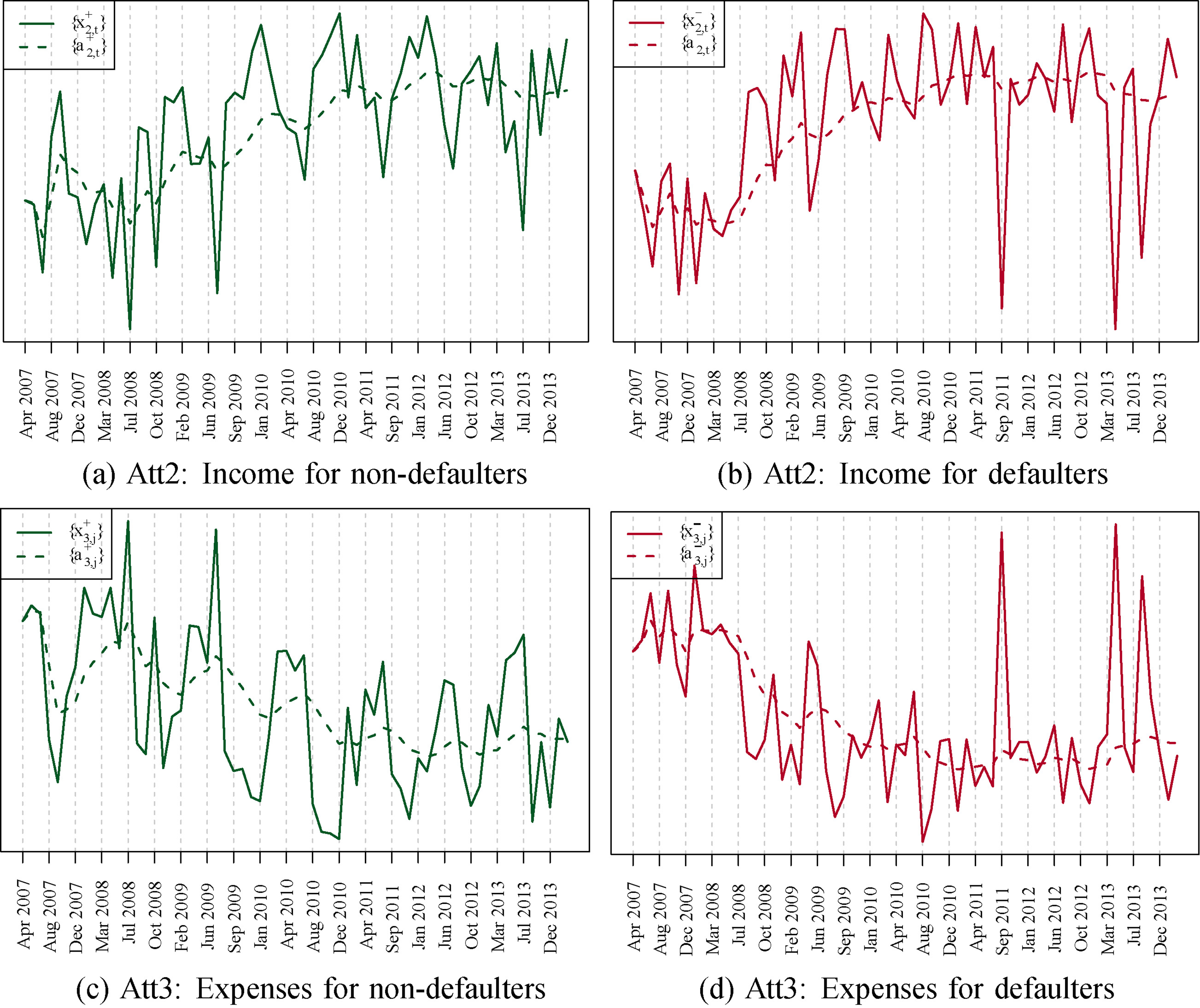
We are now interested in exploring if the changes in the tendency for all the different variables are entirely explained by the
Empirical 
In the next subsection, we show how we can extend our approach to determine if there are unexplained trends which have not been captured by our single
As for the local model, we also evaluate the robustness of the
In order to possibly identify other unexplained trends, we look at the residuals defined as the difference between the observed value and the estimated value according to the model specified in Eq. (3),
where
We then employ the same modeling approach we used in the previous sections, but now focusing on the calculated residuals. Firstly, we generate sequences of hidden variables
Secondly, we generate another sequence of hidden variables
We want to point out that this residual analysis has a straightforward interpretation in terms of multiple hidden variables. That is, an extension of the models given in Eq. (3) or Eq. (1) to include two hidden variables corresponding to
for the local model and
for the global model. In both cases,
In Fig. 7 we show the
Variances of the
Expected values of the local hidden variables for the residuals 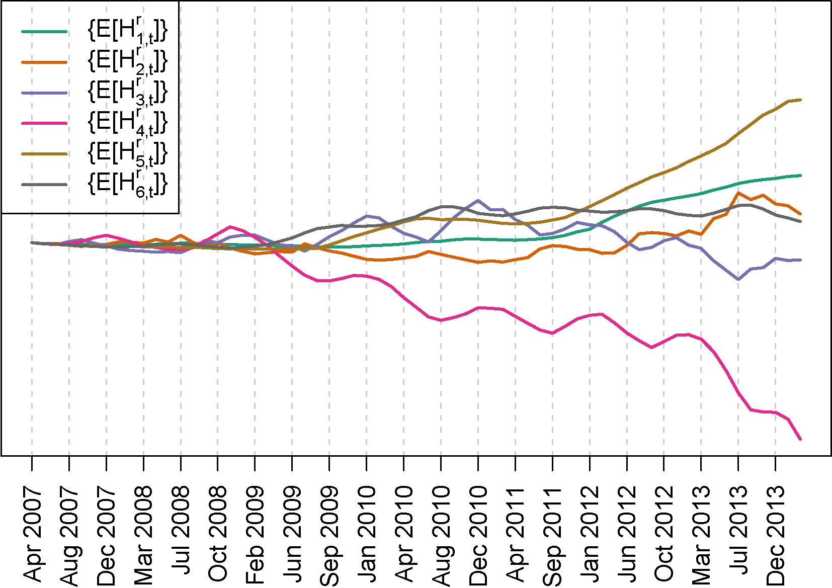
The behavior in Fig. 7 of the Account balance attribute (Att4) can partly be understood by looking at Fig. 6a. Here we can see that the Account Balance attribute has a negative trend until the end of 2008. After that time point, the Account Balance has a positive trend, which even seems to accelerate from December 2012 and until the end of the series. According to BCC’s expert, the first phase until the end of 2008 could show the progressive financial deterioration of weak non-defaulter clients in the first years of the financial crisis. The posterior increase in mean account balance would show that the clients that still remain non-defaulters are the ones with higher savings. This first phase seems to be mainly driven by the increase in the unemployment rate. This is the reason why the
Similar conclusions can be extracted for the Unpaid Mortgages attribute (Att5) by looking at Fig. 6c and the
With the above comments in mind, we can better interpret the behavior of the
The unemployment rate 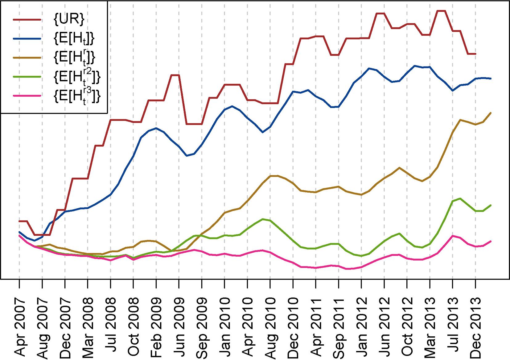
In the
The residual approach presented in the previous sections can obviously be repeated in an iterative fashion. This would be equivalent to trying to add more hidden variables for better modeling the drift of the attributes over time. In Fig. 8 we also show the result of this approach by including the
In Fig. 9, we plot the evolution of the marginal log-likelihood (this is an approximated value by variational methods, which is called the evidence lower bound (ELBO)) of the data for models with none, one, two, three, and four hidden variables. The plot shows that including a few hidden variables is enough to increase the marginal log-likelihood of the model, suggesting that increasing the model complexity beyond that point only yields small improvements.
Prequential Marginal LogLikelihood for models with different number of hidden variables.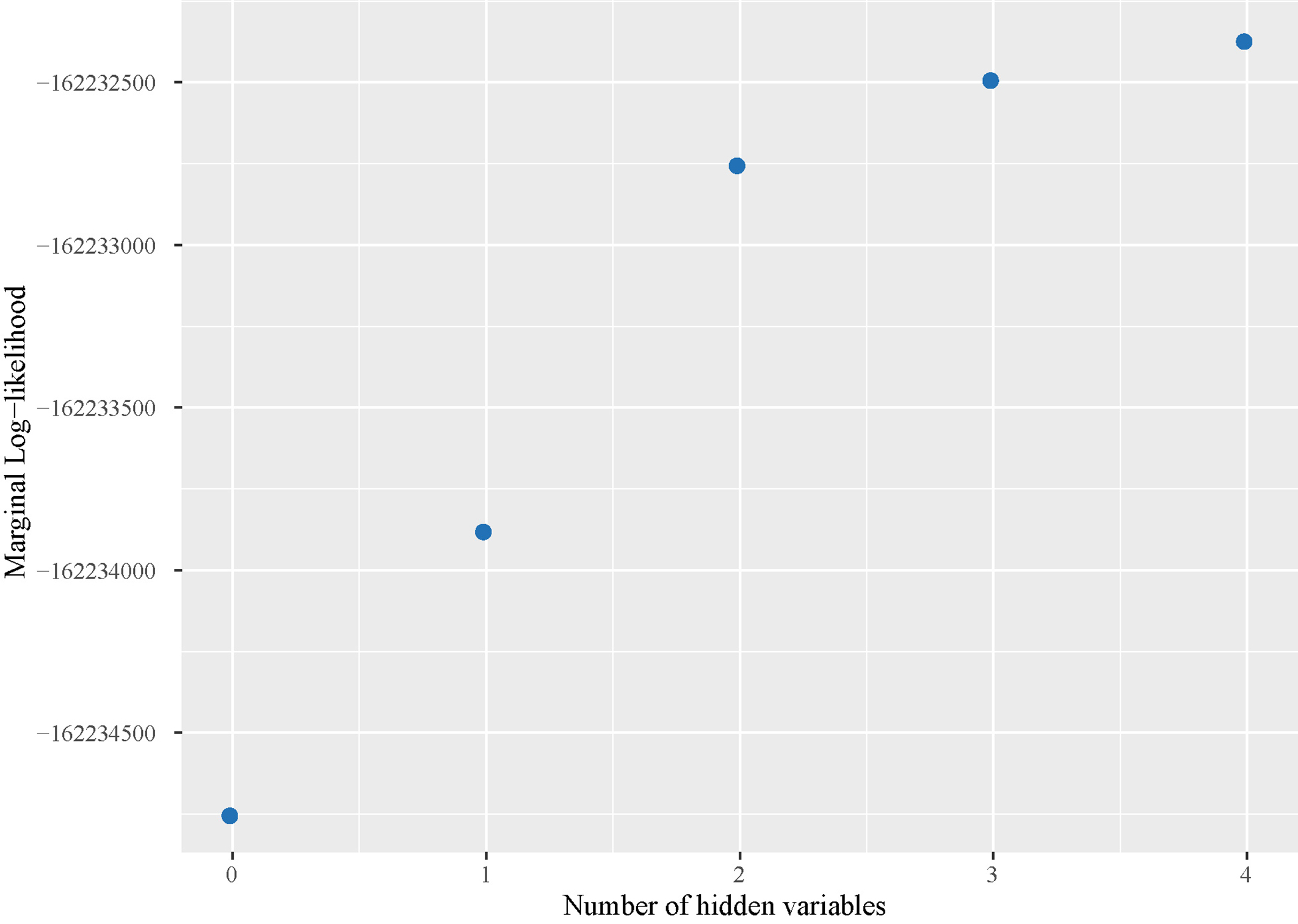
In Table 2 (Row 3), we also show the variance of the
In this section, we first want to highlight that the models used in this paper are simple instantiations of the general model family described in Section 4. For example, we are making the unrealistic assumption that the attributes are independent conditional on the defaulter status of the clients (although this is partly alleviated by the global latent variable), even when knowing that there is a strong correlation between income, expenses, and the account balance of a client. Moreover, we assume that the attributes are normally distributed, which is also an inaccurate assumption considering the histograms displayed in Fig. 2. There exist straightforward ways to alleviate the assumptions about independence and normality in distribution by explicitly linking the observed variables or using extra hidden variables and non-Gaussian distributions. Still, since our goal was to understand the underlying dynamics rather than to find a model that is a perfect fit to the data, we have not pursued this line of investigation. Instead, we have seen that even when using this simple model class we are able to obtain important insights about the general trends governing the evolution of the financial profile of the clients. In our opinion, this is a strong point in favor of the robustness of our approach.
As commented above, the proposed probabilistic concept drift model considered here is able to detect both global and local concept drift, depending on the hidden structure of the model. Additionally, the iterative process of analyzing the residuals helps reveal different levels of concept drift that may be present. For instance, different attributes may vary at different rates in opposite directions so that the trend cannot be captured by simply aggregating the local hidden variables or by using a single global hidden variable.
The presented framework can easily be extended in different directions. Computationally, the only requirement is that we choose distributions s.t. the full model is in the conjugate exponential family. Interesting alternatives include the exponential distribution (for positive real numbers with heavy tails) and the Poisson distribution (for count data). The use of more complex dependency structures between the attributes, reflecting expert knowledge, would also allow us to design more faithful models. Referring to the qualitative characterization of types of concept drift described in [22], the instantiation of the framework employed in Section 5 is specifically targeting gradual, non-reoccurring drift. This model-behaviour is to a large extent defined through the assumed prior distribution for
Another direction would be to position our concept drift analysis within a batch learning context. In such a setting, real-time analysis is not required, which means that future data can be used for making inferences about the past. In contrast, in this paper, we have pursued, following the requirements of our problem, a streaming approach, where inference is only based on past and present data. The Bayesian framework naturally supports the alternative batch approach, which we can exploit to get a more accurate global picture of our analysis. This is equivalent to the “smoothing” phase usually employed in dynamic systems with hidden variables [15].
The inherent flexibility of Bayesian latent variable models reinforces the importance of model validation. In Section 5.4 we applied a simple approach in order to study the suitability of our model. More complex evaluation procedures, which look at temporal dependencies between the residuals, would be a new line of work to validate the faithfulness of our model with respect to the analyzed data.
Conclusions
In this paper, we have used a novel model to capture different sources of concept drift in financial client data from the Spanish bank BCC. The data covers the period from April 2007 to March 2014. Despite the challenging distributions of the analyzed attributes and the simplicity of the applied model, we have been able to detect different trends that on the one hand relate to the general economic climate and on the other to the particular policies implemented by BCC during the period. The analysis is done in a streaming fashion, meaning that inferences drawn at a given point in time
The expected mean of the global concept drift variable in the model correlates almost perfectly with the unemployment rate in the region of the financial institution. It is thus natural to hypothesize that the main driving factor for concept drift is the unemployment rate, a perspective that was corroborated by a BCC expert. The analysis of the residuals has allowed us to pinpoint the attributes that do not follow the trend of the unemployment rate, mainly Account balance and Unpaid amount in mortgages. Closer analysis of these and consecutive residuals, have shown different phases in which we can see the deterioration of the non-defaulter clients on the first years of the crisis, a shift of weak non-defaulter clients to the defaulter state, and more specific actions taken by BCC, like debt restructuring and possibly a fusion with other smaller regional banks.
We have outlined future lines of research both from the point of view of the concept drift detector model and also for the practitioners.
Footnotes
Acknowledgments
The authors would like to thank BCC expert Ramón Sáez for providing valuable insights to the paper. DRL thanks the support from CDTIME (University of Almería), the research group FQM-229, and from Campus de Excelencia Internacional del Mar (CEIMAR) of the University of Almería.
Appendix
Robustness analysis
In this paper, we pursued an approach which is able to model concept drift in a streaming fashion. This approach is based on two different models: the local model described in Section 5.1 and in Eq. (1), and the global model described in Section 5.2 and in Eq. (3). In both models, we assumed that the expected values over
and this posterior therefore depends on
Expected values of the local hidden for all variables.
Expected values of the global hidden 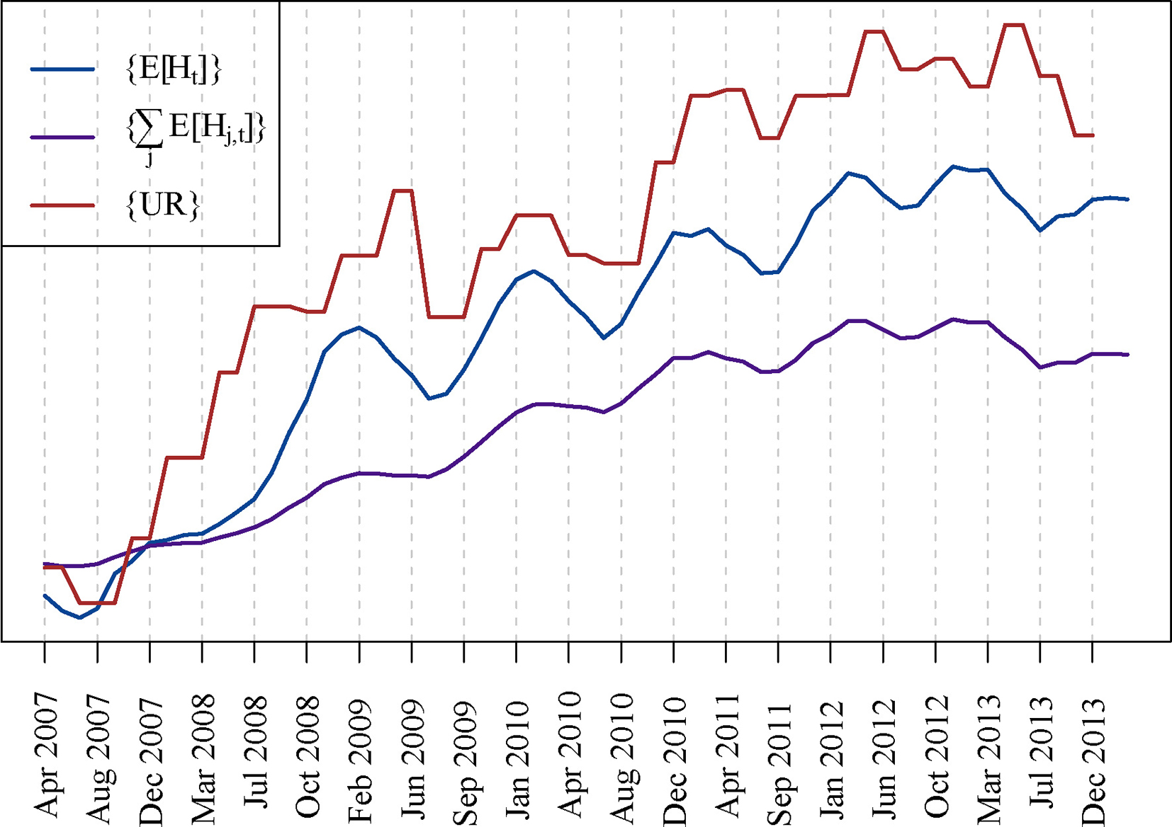
In this appendix we show that disregarding this temporal dependency of the expected values only has a marginal impact on the conclusions we draw from our interpretation of the evolution of the local and global hidden variables. In consequence, we argue that our approach can be safely used to track concept drift in a streaming fashion.
For this purpose we rerun the same experiments whose results were displayed in Figs 10 and 11 for the local and the global model, respectively. During these new experiments, all the
This setup is only intended to illustrate the marginal effect the time varying parameters have on the previous analysis. It is not being proposed as an alternative analysis method, which would haven taken the proposed method out of the streaming context.
where
In consequence, the modeling equations of the global model (cf. Eq. (3)) were rewritten as follows,
where the following entities are now assumed to be random variables according to the Bayesian formulation:
We follow the same approach to re-run the local model.
Notice how Eq. (7) takes
To this end, Figs 12 and 13 show the result of this analysis for the local and global model, respectively. In these figures we plot together the output of both approaches (with and without fixed
Series cross zero in the middle of the time series by substracting the original value. And all values are divided by the maximum of the series to guarantee a maximum value of one in each series.
Expected values 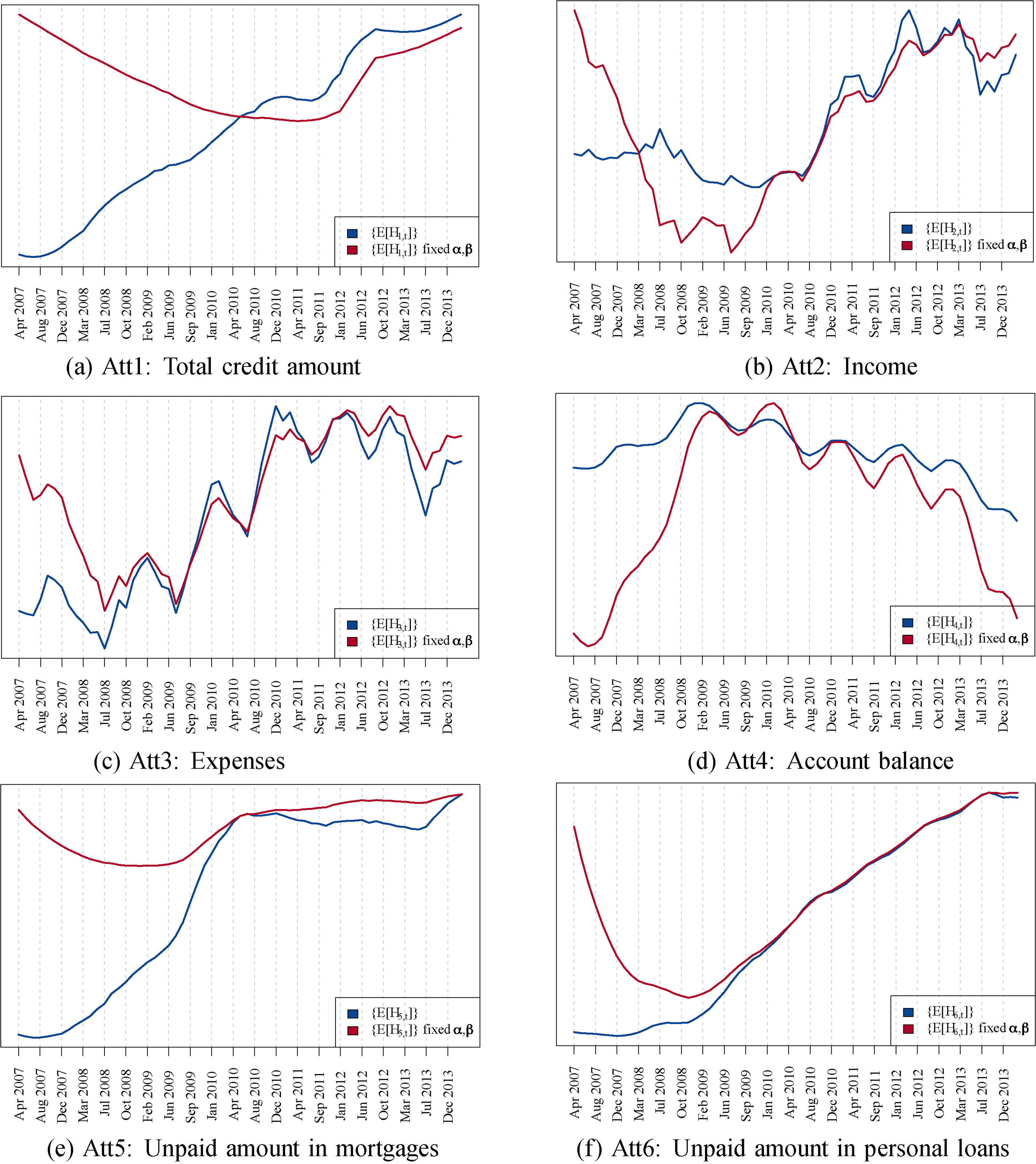
It can be appreciated that in the first months the trend captured the hidden variables (i.e.
In Table 3 we quantitatively evaluate this assessment by computing the Pearson correlation coefficient between both series (i.e. with and without fixed
Pearson Correlation coefficient between the
Series
Global
Att1
Att2
Att3
Att4
Att5
Att6
All Months
0.793
0.776
0.855
0.702
0.755
0.867
Last 2/3 Months
0.945
0.703
0.954
0.952
0.984
0.942
0.998
Expected values of the global hidden 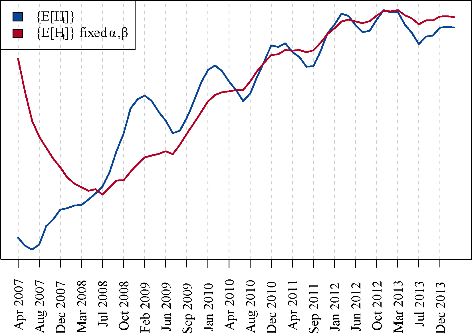
Synthetic data sets
We show how the concept drift modeling framework detailed in Section 4 can be used to analyse two synthetic data sets, widely employed as benchmarks in the concept drift literature. All the experiments have been performed using MOA [2], where the developed concept drift model (in Fig. 3) has been integrated as a new Bayesian streaming classifier, named bayes.amidstModels. The Java code to reproduce the experiments can be downloaded from