A comparative analysis of Bayesian network structure learning algorithms applied to crime data

Abstract

The theories about crime and correction have their inception in the eighteenth century, highly influenced by the anthropological thoughts emerging during the age of Enlightenment. Throughout the decades, the criminological studies observed their sociological essence encompassing practices from other scientific fields to explain the more contemporary questions, becoming Criminology an inherently interdisciplinary science as a result. The adoption of concepts from Exact Sciences is a recent moving, originating it a novel research area, called Computational Criminology, which employs procedures from Applied Mathematics, Statistics and Computer Science to provide original or enhanced solutions to such questions. One of the most prominent tasks brought by this rising field is crime prediction, which attempts to uncover potential targets for future police intervention and also help solving already committed offenses. The present comparative analysis thus investigates the employment of statistical inference by means of Bayesian network for predictive policing, using the openly accessible registers from Chicago Police Department. Numerous algorithms are available to learn the structure for a Bayesian network purely from data and a comparative examination about them is hence described, with the purpose to establish the most precise and efficient one, according to the attributes of the said criminal dataset, for the implementation of the intended inference.

Keywords

Graphical models Bayesian inference crime prediction computational statistics criminology learning algorithms

1. Introduction

In a concise definition, Criminology is the science that analyzes the nonlegal aspects of crime, from its causes and consequences to correction and prevention measures [23]. A more elucidative description comes from Edwin Sutherland, considered by many the most famous criminologist of the twentieth century, who described Criminology as the study of the making of laws, the breaking of laws and the society’s reaction to the breaking of laws [47]. Therefore, the science in its core focuses on the analysis of the crime and its perpetrators and victims as well as the criminal justice and penal systems.

Historically, the earliest criminological thoughts emerged in the pre-Enlightenment period, when people started to react to the arbitrariness and cruelty of the then systems of punishment and justice. It was only in the age of Enlightenment that the first formal principles about crime and correction were theorized, mainly of them deriving from the Classical School and its assumption that crime is the product of a deliberated choice of someone exercising free will and rationality. The offender should thus be punished according to the extent of the injuries infringed to the others by his violation [47, 41].

Under the impact of Charles Darwin’s studies on evolution of the species, in the late nineteenth century, the classical conception about crime started being intensively affected by scientific thoughts. The nature of the criminal, considered by the Classical School to be freewilled and rational, was thereby believed to be driven by biological and psychological influences, according to the ideas of the rising Positive School. The premise that factors beyond the individual’s self-control would induce him to commit the crime was one of the major critics against the positive theory, since the individual’s own responsibility in the infraction could not be taken into account by this belief [47, 41].

Several other criminological thoughts followed these two major schools of Criminology throughout the twentieth century, being the Chicago School one of the most preeminent examples. According to the idea of social ecology developed at the Department of Sociology at the University of Chicago from the First World War onwards, crime is a response to the excluding and unhealthy society in which the offender lives. Hence, understanding socio-economic contrasts helps comprehend social and geographical variation in crime and delinquency [47, 10].

With a theoretical basis explaining the essence of crime already established and in constant development, a change in the direction was a natural movement for the investigations in Criminology to fulfill the practical demands that started arising during the second half of the twentieth century. Not only the science should be concerned with what motivates a criminal incident, but also with strategies for preventing or even predicting an occurrence, opening a path to interdisciplinary studies not undertaken until then to be performed.

As a result, disciplines from Exact Sciences began to be contemplated by Criminology scholars to accomplish these more recent challenges, originating this advance a particular research area. Computational Criminology implements methods from Applied Mathematics, Statistics and Computer Science to offer original or enhanced solutions to criminological problems by means of computer-intensive applications and algorithmic procedures [7], an improvement made possible with the continuous increase in computing performance experienced in the last decades.

Thereby, operations executed in a manual mode theretofore, such as crime mapping and its pinpoint physical maps, could start being digitized. Moreover, with the aid of complex computational routines executed on more powerful machines, criminal databases comprised of thousands of millions of entries became processable, permitting the reveal of hidden qualitative information underneath them that were impossible to be noticed just by gazing at that massive amount of registers.

These advances altogether, along with many others provided by the blossom of Computational Criminology, allowed the development of novel criminological practices, being crime forecasting [50, 45] a remarkable example. By combining diverse mathematical and computational strategies, this predictive task attempts to unveil potential targets for police intervention and prevent crime [50], changing the paradigm of police action from reactive to preemptive.

Crime prediction practices may also be employed to solve already committed offenses. Through the use of statistical procedures, concealed patterns in databases of former crimes are revealed, enabling some variables of a present incident to be inferred according to its already evidenced characteristics and, consequently, orientating police strategies in the resolution of the occurrence. For example, suppose that it has been detected from past criminal records that a burglary in a certain neighborhood is usually perpetrated by a man in his twenties who lives in the industrial district. A crime prediction proceeding may tell how probable it is the offender of a newly perpetrated burglary in the same neighborhood to reside in the industrial district or even the transgression to be solved, information that gives the local police a more solid direction to the investigation of that crime.

The present article focuses on inference procedures in predictive policing practices, using Bayesian networks and the criminal records from Chicago Police Department [18]. Several algorithms are available to build a Bayesian network purely from data and a comparative analysis was implemented to establish the most precise and efficient one, depending on the attributes of that input. With the fittest Bayesian network found, inference tests were then performed to assess how robust the returned network was.

The remaining of the text is organized as follows. Section 2 conceptualizes and mathematically defines Bayesian networks. An overview of the studies that have been carried out on Bayesian network structure learning algorithms is detailed in Section 3, followed by the description of the proposed methodology for the comparison of them in Section 4 and the discussion of the experimental results obtained from the implementation of this methodology in Section 5. Section 6 presents some final remarks about the ongoing research and directions for future work regarding investigations on statistical inference within the scope of Computational Criminology.

2. Bayesian networks

Suppose that a study aiming to link the economic situation of a certain city to the oscillations of robbery rate in it was carried out, unveiling the presence of four binary-valued random variables in such scenario. Let the variable $E S$ represent the municipal economic situation; the variables $U N$ and $P S$ tell whether or not the unemployment rate and the investment in public security on that city are above 10% of the local economically active population and 2% of the local Gross Domestic Product respectively; and the fourth and last variable $R R$ symbolize the oscillation to be observed in the robbery rate in the city according to the configuration of the other three variables.

Since the considered variables are all binary-valued, an extensively calculation of the joint probability distribution $p_{R}(ES,UN,PS,RR)$ over these four variables for the robbery rate problem $R$ , that is, the table in which each row represents a specific instantiation of that set and the probability of it to occur, would demand fifteen values to be stored. Thus, straightforwardly, for the simplest cases where the problem is entirely modelled by $N$ binary random variables, $2^{N}-1$ probabilities would be needed to completely describe its joint distribution, an infeasible practice as $N$ grows or in the events of multivariate variables.

Probabilistic graphical models, or simply graphical models, combine knowledge from the fields of Graph Theory, Statistics and Computer Science to provide a generally more compact and efficient framework of a joint probability distribution, which is achieved by contemplating only the dependences between the random variables of the problem for the construction of the probabilistic model [58]. A graph is the usual structure underneath a graphical model, representing the random variables by its vertices or nodes and the statistical relationships between the variables by the presence or absence of edges connecting the nodes that depict them. Therefore, graphs offer a more intuitive way of understanding and abstracting out the conditional independence relations inherent to the problem, a commonly impracticable task by only analyzing the joint distribution table and its probabilities.

The possible structures of the graph underneath a graphical model may be diverse, according to its dynamic and the nature of its edges and random variables [58]. The cases where the graph is acyclic and has only directed edges, or arcs, represent a special class of graphical models called Bayesian networks [40, 51]. Mathematically, a Bayesian network $\mathcal{B}=(\mathbf{V},\mathbf{A},\mathbf{\Theta})$ is fully characterized by the $n_{\mathbf{V}}$ -sized set of nodes $\mathbf{V}$ , representing the $n_{\mathbf{V}}$ distinct random variables of the modelled problem, each one with a particular finite sample space containing mutually exclusive states; the set of arcs $\mathbf{A}$ between the nodes; and the set of parameters $\mathbf{\Theta}$ , described by a conditional probability table over the nodes of the graph. Under this notation, the joint probability distribution $p(X_{1},X_{2},\ldots,X_{n_{\mathbf{V}}})$ for the Bayesian network $\mathcal{B}$ is given by

$\displaystyle p(X_{1},X_{2},\ldots,X_{n_{\mathbf{V}}})=\prod_{i=1}^{n_{\mathbf% {V}}}p(X_{i}|\Pi_{i})$ (1)

where $p(X_{i}|\Pi_{i})$ is the conditional probability for the node $X_{i}\in\mathbf{V}$ given the set $\Pi_{i}\subset\mathbf{V}\setminus X_{i}$ of all parent nodes of $X_{i}$ , that is, the nodes connected to $X_{i}$ by an arc with $X_{i}$ in its tail.

Bringing back the initial example, suppose, then, that a Bayesian network $\mathcal{B}_{R}=(\mathbf{V}_{R},\mathbf{A}_{R},\mathbf{\Theta}_{R})$ for the robbery rate problem $R$ was built by an expert in crime studies, who was able to unveil the independence relations between the previously presented variables from his expertise, which is depicted in Fig. 1. From this network, it is thus possible to abstract out that the municipal economic situation directly influences the unemployment rate and the investment in public security in the city, as variable $E S$ is a parent node of both variables $U N$ and $P S$ . Both of these, in turn, being parent nodes of variable $R R$ , have a direct impact on the local robbery rate, which is also indirectly affected by the economic situation of the city, since $E S$ is a parent node of the parent nodes of $R R$ .

Figure 1.

Bayesian network for the robbery rate problem.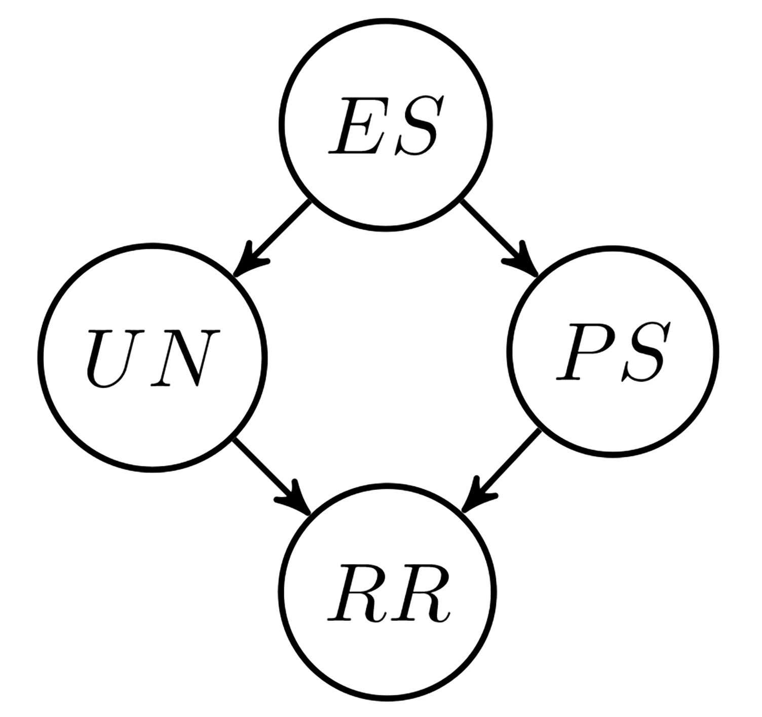

From Eq. (1) and Fig. 1, the joint probability distribution $p_{R}$ for the robbery rate problem $R$ is then expressed by

$\displaystyle p_{R}(ES,UN,PS,RR)=p_{R}(ES)\cdot p_{R}(UN|ES)\cdot p_{R}(PS|ES)% \cdot p_{R}(RR|UN,PS)$ (2)

from which the cardinality of the set of parameters $\mathbf{\Theta}_{R}$ can be determined, factor by factor. Since it is the marginal probability for the root node $E S$ in the network $\mathcal{B}_{R}$ , the first factor $p_{R}(ES)$ requires only one parameter to be stored, more precisely, the probability for one of the two possible states of the binary-valued variable $E S$ , since the probability for the other one may be directly calculated by the basic probability property $p(X=x_{1})=1-p(X=x_{2})$ , for any binary random variable $X$ .

Following similar reasoning, the second factor demands two parameters to be kept, determined by the values of the conditional probability $p_{R}(UN|ES)$ calculated for a fixed value of the variable $U N$ , given the two possible states of the variable $E S$ , one at a time; the same logic is applied to $p_{R}(PS|ES)$ . In addition, for the fourth and last factor $p_{R}(RR|UN,PS)$ , four parameters are needed in an analogous and straightforward way, summing up a total of nine values to be stored, instead of the original fifteen ones, a slight saving in storage that would be significantly greater in larger and more complex problems.

In this example, the cardinality of the set of parameters $\mathbf{\Theta}_{R}$ was established over a Bayesian network hypothetically built by an expert on the problem domain. Nevertheless, it is not always possible to count on the expertise of a third party for such work and one must make use of practical ways of inferring the desired graph underlying the data to deduce the corresponding conditional probabilities. Structure learning algorithms fulfill this role, as statistical procedures designed to determine, generally in an automatic manner, which model or graph is the most suitable to encode the dependences between the variables of the input data. Various methods that have been developed for the indicated purpose are described in Section 3 and a comparative analysis, applied to crime data, of some of the most notable is in the core of the methodology to be presented in Section 4.

3. Related work

Modeling real-life problems for reasoning under uncertainty with Bayesian networks used to rely solely upon domain knowledge. Generally, such expert systems were constructed from comprehension obtained with human specialists, a task found to be computational and financially expensive and also highly susceptible to errors [39]. Automating this process of building knowledge for a fully-automated model construction routine was the solution encountered to overcome these issues, a paradigm shift that allowed Bayesian networks to gain notability outside academia and be widely applied in many different fields [58, 51, 39].

Among the most prominent earlier methods developed to learn a Bayesian network purely from data is PC (named after its authors, Peter and Clark [57]), which employs order-increasing conditional independence tests in the set of the problem variables to find, starting from an initial complete graph, the skeleton of the network, thereby reducing the adjacencies between nodes and consequently improving the running times in the following edge-orienting steps [44]. The continuously-growing high dimensionality of the manipulated datasets motivated the development of more efficient learning algorithms, such as Grow-Shrink [44], which implements the conditional independence tests over the Markov blankets computed for each variable in the set instead, making the structure discovery phase faster.

Several other methods were later devised to mainly enhance these ideas. Incremental Association and its variants [61, 67] focused on strengthening the heuristic used to uncover the Markov blankets from Grow-Shrink, in order to avoid variables to be incorrectly attributed to a specific blanket and that would have to be removed in a later stage, augmenting the overall performance time. PC-stable [20] modified the skeleton building phase from PC to resolve the order-dependence supposedly inherent to it that would lead the resulting Bayesian network to depend on the order in which the variables were evaluated during that step. MPC [60], in turn, left the original skeleton building phase unchanged and adjusted the edge-orienting rules to effectively prevent cycles. Parallel-PC [42] incorporated parallelization techniques to improve both the efficiency and accuracy of the conditional independence tests.

In a general framework, all the aforementioned algorithms initially unveil the undirected graph underlying the Bayesian network to be constructed by means of conditional independence tests, or constraints, and then orient the edges of the graph in a sequence of subsequent steps. Employing statistical tests as their typical routines have thus led these methods to be known as constraint-based structure learning algorithms. Score-based algorithms comprise a second group of structure learning methods that obey a more compact framework, by which a series of directed acyclic graphs is constructed and a score for each of them is assigned by a prior specified score function, being selected the graph that maximizes that value, that is, the network with the highest score. This procedure clearly reduces the structure learning exercise to a simpler search problem [46, 36].

Being the search space superexponential in the number of nodes of the Bayesian network to be constructed, an exhaustive evaluation of all candidate networks by a score-based method is thus unfeasible. A primary practice to address this issue would be reducing the size of the search space with the assistance of domain experts, who could establish which nodes were certainly connected and also the direction of the arcs between them [58]. Since expert knowledge is often a resource not easily available, heuristic strategies are regularly implemented as the main nonextensive alternative to tackle the search space size problem in a score-based learning process [36, 43].

Hill Climbing [52], also known as Greedy Local Search, is a heuristic commonly performed for such purpose, by which the search starts from an initial position and continually advances in the direction of increasing value of the evaluated function, until no higher values are obtained. In the context of Bayesian network structure learning, such strategy usually begins with an empty network, or a structure suggested by an expert in the problem domain, and carries out arc operations that do not result in a cyclic network, by adding, removing or reversing the direction of a single arc at a time, until the score assessed to the network obtained from these operations is no longer improved.

The structure returned by this routine may be a local and not a global optimum, though, as it regularly happens with heuristic search algorithms. One widely-known technique to overcome this drawback is to reinitialize the search with an initial state randomly generated after a fixed amount of iterations is completed, being selected the network with the maximum score throughout the whole process [36, 52]. Another popular approach is Tabu Search [29], which keeps a fixed-numbered tabu list of previously visited states that are forbidden to be revisited, allowing the search to escape from local minima and improving the heuristic efficiency as well [52].

For the score evaluation to guide the aforesaid search proceeding, various notable functions have been developed. Akaike Information Criterion [1], Bayesian Information Criterion [53] and Mutual Information Test [21] are examples of information-theoretic-based score functions, while K2 [39], Bayesian Dirichlet and its variants [33, 12, 59, 54] rely on Bayesian computation of posterior probability distributions. Practical guidelines recommend using the functions from the former group with large datasets and those from the latter with small ones [11], although it is not a strict rule.

This search-and-score strategy inherent to score-based algorithms, combined with the conditional independence tests routine intrinsic to the constraint-based ones, constitutes a third category of structure learning methods, called hybrid algorithms. In the first phase of their common two-stage single procedure, a restrict proceeding reduces the set of possible parents of each node in the graph through independence statistical tests, thus lessening the search space of candidate networks or even providing a basic network to work as a seed in the second stage, which seeks to maximize a predetermined score function, evaluated for all the structures in the restricted set returned by the first stage [46, 43].

The routines executed in each of these two stages depend on the hybrid algorithm chosen. A remarkable example is Max-Min Hill Climbing [63], that runs the Max-Min Parents and Children [62] and Hill Climbing algorithms in the restrict and search stages respectively. A more recent hybrid method, called Hybrid HPC [25], employs constraint-based Hybrid Parents and Children [22] to reconstruct the skeleton of the Bayesian network and score-based Hill Climbing to orient the edges, an association that outperforms Max-Min Hill Climbing in terms of goodness of fit and quality of the network structure [25].

Even though such a diversified number of methods has already been developed, the research area of structure learning algorithms is continuously receiving novel contributions. The fact that both Integer Linear Programming and Bayesian network structure learning are NP-complete [13, 24, 49] drove the usage of techniques from the former to encode problems from the latter as an integer linear optimization problem [5, 6]. Evolutionary algorithms, for instance, Particle Swarm Optimization [26, 66, 56], Cuckoo Search [4, 8] and Ant Colony Optimization [69, 68], among others, have been applied to enhance the search routines in score-based learning methods. Remarkable contributions also come from studies employing Simulated Annealing [48, 34] and Learning Automata [27, 28] procedures. These examples show that Bayesian network structure learning remains a research area open to the fostering of more solutions, either original or improved ones, and thus constantly reckoning on comparative analysis of the developed methods so far for further advancements.

4. Methodology

The methodology employed by the present analysis starts with a data processing step, in which the input is treated by means of data conversion and selection. The processed data then feeds the Bayesian network validation and construction stages, executed both for each structure learning method considered for examination, assessing this proceeding the metrics and graphs to be used by the intended global comparison evaluation. With the most dependable learning algorithm eventually ratified, the data goes through another processing step to extract the subset over which the final model is to be validated and constructed by the established method. After an occasional refinement stage, statistical predictions are then carried out using the definitive model, as a final step. This methodological flowchart is illustrated in Fig. 2.

Figure 2.

Methodological flowchart.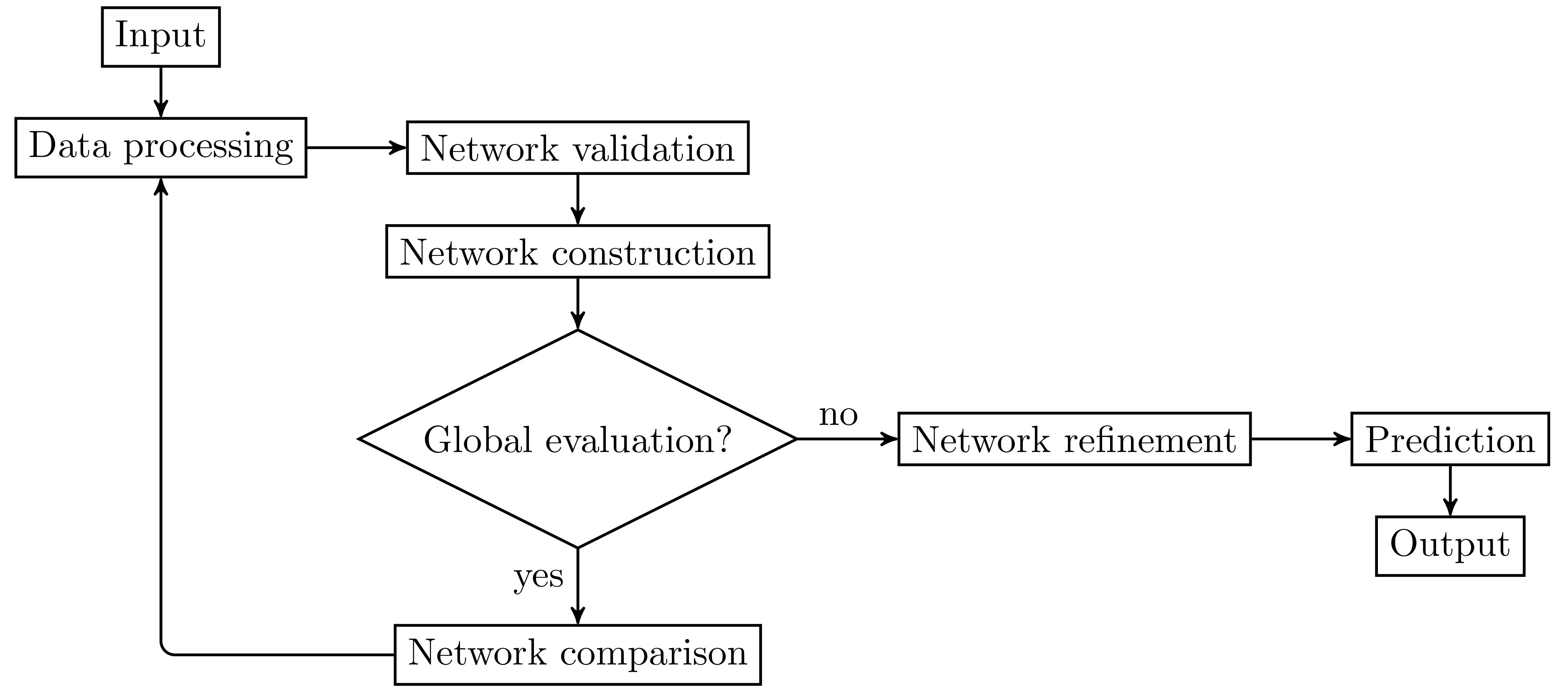

Although devised to describe a fully-automated Bayesian network structure learning routine, domain experts may play a key role during the execution of the methodology described above, for more reliable results. Such part is explained in the next subsections, along with a more detailed exposition of each aforementioned methodological stage.

4.1 Input and data processing

For the input data, among the criminal records openly provided by police departments from some of the biggest metropolitan cities throughout the globe, such as London [30] and San Francisco [14], those from Chicago Police Department [18] were chosen, as they are more detailed in comparison with the others and include Boolean fields susceptible to be worked as the decision variables for the intended Bayesian networks.

Structurally, the Chicago Police Department dataset comprises more than six million rows, each row representing a reported crime from 2001 to present and characterized by twenty-two descriptive columns. Among these fields, there are two working as unique identifiers for the criminal record; one for the best estimated date and time when the incident occurred and another one for the year; seven depicting, physical and geographically, the location where the crime happened; four locating the occurrence in different sectional divisions of Chicago city; four describing the type of crime; two indicating, in a Boolean manner, whether or not an arrest was made or the incident was domestic-related; and one for the date and time when the record was last updated.

For the global comparison stage, in which different-sized Bayesian networks are built and evaluated in terms of fitting errors and construction times, nine of these twenty-two columns were removed, either for them being mostly empty or representing variables with meaningless information, such as the ID number particular to each register. The data in all of the thirteen remaining columns were handled in their original form, with exception made for the one contained in the field Date, indicating the best estimated date and time when the incident occurred, that was processed to situate the crime in one of the five different parts of the day and renamed to Part.

The criminal records containing blank fields, that is, not completely filled during the register of the occurrence, were likewise discarded, since imputing arbitrary values to complete these faulty records could bias the results. Lastly, the whole dataset was restricted to the period between 2015 and 2017, from the idea that crime, being influenced by the natural non-static social conjuncture where it happens, shows a dynamic behavior over time and so it is more significantly affected by events from short-term past.

Thus, in the data processing step, the comma-separated values file containing the reported crimes obtained from Chicago Police Department goes through a dimensionality reduction by means of field selection, followed it by a data treatment and a sequential temporal constriction to the most recent years. Once this procedure is done, the processed file is then read by a computational routine into a data structure suitable to feed the Bayesian network validation and construction stages.

4.2 Bayesian network validation

Several well-established methods are available to build a Bayesian network purely from data, making the assessment of their performance a necessary practice to choose the best one [32]. For this purpose, the input data is randomly split into two mutually exclusive sets, namely, the training set, employed to fit the cogitated models to the data, and the validation set, applied to estimate the error between the instances of this set and their respective predicted values returned by the trained models.

Although theoretical and computationally simple, the error estimated by this routine depends on the way the data is split into the training and the validation sets and may thus highly vary from one division to another [35]. Cross-validation is a traditional strategy commonly used to address this issue that can be applied to almost any structure learning algorithm, as it relies only on the assumption that the input data are independent and identically distributed [3].

Among all cross-validation techniques provided by literature, one of the most widely implemented is $k$ -fold cross-validation. This approach randomly breaks the data into $k$ groups or folds of approximately equal size, holding one fold out so the model is trained using the remaining $k-1$ ones. The isolated group then works as the validation set to estimate the fitting error of the constructed model. In each one of the $k$ executions of the described procedure, a completely different fold is selected as the validation set, so that the overall loss of the cross-validated model is computed by averaging the values of the $k$ distinct losses determined throughout the process.

These $k$ fitting errors are estimated through a predefined loss function. Once again, many options are largely available, being the log-likelihood loss $L$ , also known as negative entropy, a long-established one, which expression is given by

$\displaystyle L=-\text{argmax}_{\mathbf{\Theta}}\sum_{i=1}^{n}\log{p(\mathbf{d% }_{i}|\mathbf{\Theta})}$ (3)

where $\mathbf{d}_{i}$ , $\mathbf{\Theta}$ and $p(\mathbf{d}_{i}|\mathbf{\Theta})$ are the $i$ -th entry in the $n$ -sized input data $\mathbf{D}$ , the set of model parameters to be determined and the likelihood function respectively [9].

Bringing Eq. (3) into Bayesian network $k$ -fold cross-validation framework for the assessment of the structure learning algorithm $\mathcal{A}$ , let

$\displaystyle L_{(k,\mathcal{A})}^{j}=-\text{argmax}_{\mathbf{\Theta}_{j}}\sum% _{i=1}^{t}\log{p_{\mathcal{A}}(\mathbf{t}_{i}|\mathbf{\Theta}_{j})}$

be the log-likelihood loss calculated in the $j$ -th iteration, $1\leqslant j\leqslant k$ , from a $t$ -sized training set $\mathbf{T}$ . The overall loss $L_{(k,\mathcal{A})}$ for the network constructed by $\mathcal{A}$ is eventually determined by

$\displaystyle L_{(k,\mathcal{A})}=\frac{1}{k}\sum_{j=1}^{k}L_{(k,\mathcal{A})}% ^{j}$

being the most suitable structure learning method, for the given data, the one with the lowest $L_{(k,\mathcal{A})}$ .

Regarding how to appropriately choose the parameter $k$ , the variance and bias of the networks cross-validated by different values of $k$ have to be taken into account. Variance measures how much the model would change if it was estimated using a different training set, while bias refers to the error introduced into the parameters by representing a usually extremely complex real-life problem by a simpler statistical model. An ideal one has both low variance and low bias, a feature generally hard to achieve in practice, so a trade-off between those two attributes must be done. For this, it has been already empirically shown that moderate values of $k$ , say $k=5$ or $k=10$ , yield loss estimates that accomplish such exchange, that is, which are not affected by excessively high bias or excessively high variance [35, 38].

Additional qualitative constraints, provided by expert knowledge, may be incorporated into the validation process to elicit the model parameters, or some of them, and consequently generate a more dependable primary network for the following methodological steps, especially in cases where there is insufficient data. Nevertheless, such practice could bias the structure to be constructed and methods to minimize the risk of errors resulting from it are usually infeasible for larger problems [31, 65]. Since the present study focused on a fully-automated structure learning methodology performed on a robust input dataset, this approach was not considered.

That all explained, the Bayesian network validation step generates random subsets of the processed input data at first, differing them solely in the number $N$ of the descriptive fields contained in each corresponding subdata $\mathbf{S}$ , that is, in the cardinality of the network to be validated over each of them, while maintaining the total of registers for them all. For every subset, a $k$ -fold cross-validation is then implemented for five different values of $k$ , ranging from 5 to 25, and nine distinct structure learning algorithms $\mathcal{A}$ , which are going to be specified in Subsection 4.3, returning this procedure a graph of the size $N$ versus the mean of the overall losses $L_{(k,\mathcal{A})}$ , plotted for each learning method $\mathcal{A}$ , as one of the metrics for the Bayesian network comparison step.

4.3 Bayesian network construction

With the purpose to offer a broad comparative analysis of the most prominent available structure learning algorithms, methods from all the three categories theoretically introduced in Section 3 were investigated in the present study. Therefore, the mathematical rules shared in common by the algorithms in each group are explained below, for a better comprehension of the work done.

4.3.1 Constraint-based algorithms

As described in Section 3, the techniques in the first category of structure learning algorithms essentially rely on statistical tests carried out on the dataset. Thereby, let $\mathbf{V}$ be the set of random variables in the input $\mathbf{D}$ . Then, for each possible triple $(X,Y,\mathbf{S})$ , where $X,Y\in\mathbf{V}$ and $\mathbf{S}\subset\mathbf{V}\setminus\{X,Y\}$ , a statistical test, usually a conditional independence one, is executed to check whether or not $X$ is independent from $Y$ given $\mathbf{S}$ or, in mathematical notation, if $X\bot Y|\mathbf{S}$ .

For these conditional independence constraints, the chi-squared test $\chi^{2}$ is a classic one, being it a function of the observed frequencies of every possible configuration for the triple $(X,Y,\mathbf{S})$ . Supposing that $\mathbf{S}$ is a single-valued subset, that is, $\mathbf{S}=\{Z\}\subset\mathbf{V}$ , and considering that $n_{X}=|\mathbf{\Omega}_{X}|$ , $n_{Y}=|\mathbf{\Omega}_{Y}|$ and $n_{Z}=|\mathbf{\Omega}_{Z}|$ , where $\mathbf{\Omega}$ is the sample space of the subscripted variable, then

$\displaystyle\chi^{2}(X,Y|\mathbf{S})=\chi^{2}(X,Y|Z)=\sum_{i=1}^{n_{X}}\sum_{% j=1}^{n_{Y}}\sum_{k=1}^{n_{Z}}\frac{(o_{\textit{ijk}}-e_{\textit{ijk}})^{2}}{e% _{\textit{ijk}}}$ (4)

expression straightforwardly extensible to the cases where $\mathbf{S}$ contains more than one random variable.

In Eq. (4), the minuend $o_{\textit{ijk}}$ is the observed frequency of the triple $(X,Y,Z)=(x_{i},y_{j},z_{k})$ in the $n$ -sized input dataset $\mathbf{D}$ , with $x_{i}\in\mathbf{\Omega}_{X}$ , $y_{j}\in\mathbf{\Omega}_{Y}$ and $z_{k}\in\mathbf{\Omega}_{Z}$ , and simply determined by the ratio between the number of observed instances of the referred configuration in $\mathbf{D}$ and the size $n$ . The quantity $e_{\textit{ijk}}$ , in turn, is the expected frequency for the same triple and calculated by

$\displaystyle e_{\textit{ijk}}=\frac{n_{i\cdot k}\cdot n_{\cdot jk}}{n_{\cdot% \cdot k}}$

where the factors are computed according to the sums

$\displaystyle n_{i\cdot k}=\sum_{j=1}^{n_{Y}}o_{\textit{ijk}},\quad n_{\cdot jk% }=\sum_{i=1}^{n_{X}}o_{\textit{ijk}}\quad\textrm{and}\quad n_{\cdot\cdot k}=% \sum_{i=1}^{n_{X}}\sum_{j=1}^{n_{Y}}o_{\textit{ijk}}$

over the observed frequencies $o_{\textit{ijk}}$ [46, 64].

The afore-explained chi-squared test $\chi^{2}$ , as the chosen conditional independence test for all the constraint-based learning routines implemented by the methodology (specifically, PC, Grow-Shrink, Incremental Association and its fast and interleaved variants), is executed during the first phase of Algorithm 4.3.1, that focuses on generating an initial skeleton for the Bayesian network $\mathcal{B}$ and where $\mathbf{N}_{X}$ denotes the neighborhood of node $X$ . For that purpose, the network $\mathcal{B}$ is initialized with a complete graph $K_{n_{\mathbf{V}}}$ , $n_{\mathbf{V}}=|\mathbf{V}|$ , and through removing the edges between the unveiled conditional independent variables, the intended skeleton is then output [19].

A two-step edge-orienting procedure follows this graph-constructing stage, starting by detecting the v-structures present in the graph. According to this topological pattern, every set of three variables $\{X,Y,Z\}\subset\mathbf{V}$ , with $X$ and $Y$ adjacent to $Z$ , but not to each other, has its edges oriented so that both $X$ and $Y$ become parent nodes of $Z$ . In case there are remaining unoriented edges after this proceeding, their directions are finally established following further topological rules, that guarantee that no cycles or additional v-structures are created from the orientation of those edges, after what the directed acyclic graph depicting the Bayesian network $\mathcal{B}$ is eventually returned [19].

Essential framework for constraint-based structure learning methods[1] initialize $\mathcal{B}=(\mathbf{V}_{\mathcal{B}}=\mathbf{V},\mathbf{E}_{\mathcal{B}})% \leftarrow K_{n_{\mathbf{V}}}$ , $\mathbf{A}_{\mathcal{B}}\leftarrow\varnothing$ and $i\leftarrow 0$ initialize $\Gamma_{X,Y}\leftarrow\varnothing$ , $\forall(X,Y)\in\mathbf{V}\times\mathbf{V}|X\neq Y$ ( $X\in\mathbf{V}_{\mathcal{B}}$ ) ( $Y\in\mathbf{N}_{X}$ ) choose $\mathbf{S}$ such that $\mathbf{S}\subseteq\mathbf{N}_{X}\setminus Y$ and $|\mathbf{S}|=i$ ( $X\bot Y|\mathbf{S}$ ) delete $e_{XY}$ from $\mathbf{E}_{\mathcal{B}}$ store $\mathbf{S}$ in both sets $\Gamma_{X,Y}$ and $\Gamma_{Y,X}$ ( $e_{XY}$ is not deleted and all possible subsets $\mathbf{S}$ have not been chosen) update $i\leftarrow i+1$ ( $|\mathbf{N}_{X}\setminus Y|\geqslant i$ ) ( $\{X,Y,Z\}\subset\mathbf{V}_{\mathcal{B}}$ such that $e_{XZ},e_{YZ}\in\mathbf{E}_{\mathcal{B}}$ and $X\notin\mathbf{N}_{Y}$ ) ( $Z\notin\Gamma_{X,Y}$ ) add $a_{XZ},a_{YZ}$ to $\mathbf{A}_{\mathcal{B}}$ delete $e_{XZ},e_{YZ}$ from $\mathbf{E}_{\mathcal{B}}$ ( $\{X,Y,Z\}\subset\mathbf{V}_{\mathcal{B}}$ such that $a_{XY}\in\mathbf{A}_{\mathcal{B}}$ , $e_{YZ}\in\mathbf{E}_{\mathcal{B}}$ and $X\notin\mathbf{N}_{Z}$ ) add $a_{YZ}$ to $\mathbf{A}_{\mathcal{B}}$ delete $e_{YZ}$ from $\mathbf{E}_{\mathcal{B}}$ ( $\{X,Y\}\subset\mathbf{V}_{\mathcal{B}}$ such that $e_{XY}\in\mathbf{E}_{\mathcal{B}}$ and $\exists$ a directed path $P$ from $X$ to $Y$ ) add $a_{XY}$ to $\mathbf{A}_{\mathcal{B}}$ delete $e_{XY}$ from $\mathbf{E}_{\mathcal{B}}$ ( $\mathbf{E}_{\mathcal{B}}\neq\varnothing$ ) update $\mathcal{B}\leftarrow\mathcal{B}=(\mathbf{V}_{\mathcal{B}}=\mathbf{V},\mathbf{% A}_{\mathcal{B}})$ $\mathcal{B}$

Essential framework for score-based structure learning methods[1] initialize $\mathcal{B}=(\mathbf{V}_{\mathcal{B}}=\mathbf{V},\mathbf{A}_{\mathcal{B}}=\varnothing)$ , $\mathcal{B}_{\textit{current}}\leftarrow\varnothing$ and $\textit{score}_{\textit{max}}\leftarrow\textit{score}(\mathcal{B})$ store in $\mathcal{B}_{\textit{current}}$ the result of a single arc operation on $\mathcal{B}$ ( $\textit{score}(\mathcal{B}_{\textit{current}})>\textit{score}_{\textit{max}}$ ) update $\mathcal{B}\leftarrow\mathcal{B}_{\textit{current}}$ update $\textit{score}_{\textit{max}}\leftarrow\textit{score}(\mathcal{B}_{\textit{% current}})$ ( $\textit{score}(\mathcal{B}_{\textit{current}})>\textit{score}_{\textit{max}}$ ) $\mathcal{B}$

4.3.2 Score-based algorithms

The algorithms belonging to the second group of learning methods are ruled by a comparatively simpler search-and-score framework, presented in Algorithm 4.3.1 and which follows what was previously stated in Section 3. For the score function inherent to this strategy, among all the ones introduced earlier, the Bayesian Information Criterion, also known as Schwarz Criterion, was the methodological choice for both score-based learning routines evaluated, namely, Hill Climbing and Tabu Search.

To mathematically represent the criterion, denote the Bayesian network to be evaluated by $\mathcal{B}$ , the $n$ -sized input data by $\mathbf{D}$ and the set of random variables in $\mathbf{D}$ , or the set of nodes in $\mathcal{B}$ likewise, by $\mathbf{V}=\{X_{1},X_{2},\ldots,X_{n_{\mathbf{V}}}\}$ . Also, let $n_{i}$ be the cardinality of the sample space $\mathbf{\Omega}_{X_{i}}$ , let $\mathbf{\Pi}_{i}$ be the subset of $\mathbf{V}\setminus X_{i}$ containing the parent nodes of $X_{i}$ and let the product

$\displaystyle q_{i}=\prod_{X_{p}\in\mathbf{\Pi}_{i}}n_{p}$

be the total number of configurations over the variables in $\mathbf{\Pi}_{i}$ , fixing $q_{i}=1$ if $X_{i}$ has no parents in $\mathcal{B}$ . The Bayesian Information Criterion, generally referred to by its acronym BIC, is then expressed by

$\displaystyle\textit{BIC}(\mathcal{B}|\mathbf{D})=\sum_{i=1}^{n_{\mathbf{V}}}% \sum_{j=1}^{q_{i}}\sum_{k=1}^{n_{i}}\left[D_{\textit{ijk}}\cdot\log_{2}{\left(% \frac{D_{\textit{ijk}}}{D_{ij}}\right)}\right]-\frac{\log_{2}{n}}{2}\sum_{i=1}% ^{n_{\mathbf{V}}}q_{i}(n_{i}-1)$

where the dividend $D_{\textit{ijk}}$ is the amount of instances in the input dataset $\mathbf{D}$ , with $\mathbf{\Pi}_{i}$ and $X_{i}$ in the $j$ -th and $k$ -th configurations respectively. The divisor $D_{ij}$ , in turn, is calculated by the summation

$\displaystyle D_{ij}=\sum_{k=1}^{n_{i}}D_{\textit{ijk}}$

that is, $D_{ij}$ is the number of entries in $\mathbf{D}$ having the product $\mathbf{\Pi}_{i}$ fixed in its $j$ -th setup, for each possible state of the variable $X_{i}$ . The fittest Bayesian network to represent the independence relations between the random variables of the input data is thus the one with highest Bayesian Information Criterion score, among all the directed acyclic graphs generated by the greedy search procedure.

4.3.3 Hybrid algorithms

From Section 3, the methods in the third category of learning algorithms are a hybrid combination of constraint-based conditional independence tests routines and score-based search-and-score strategies. For the present comparative analysis, both Max-Min Hill Climbing and Hiton Hill Climbing methods were executed, the latter being an informal naming of a hybrid implementation of Hiton Parents and Children [2] and Hill Climbing algorithms.

4.3.4 Construction evaluation

The time spent to structure the Bayesian network $\mathbf{B}$ over every subset $\mathbf{S}$ , as established in Subsection 4.2, is the metric assessed in this step of the methodology, considered it to be relevant once the size of the manipulated criminal dataset, comprised of hundreds of thousands of records, is taken into account. Five measurements of construction time are thus performed, per learning algorithm $\mathcal{A}$ and subset $\mathbf{S}$ , in order to produce a qualitative graph of the corresponding mean time versus the size $N=|\mathbf{S}|$ , for each method $\mathcal{A}$ .

4.4 Bayesian network comparison

With all the metrics finally estimated, a performance comparison of all learning methods is then executed, to define the most suitable one. From the losses retrieved in Subsection 4.2, it is possible to determine which algorithm returns the lowest fitting error on average; from the time measurements quantified in Subsection 4.3, the average efficiency of each learning method may be established.

In addition to these examinations, the effectiveness of each learning algorithm may also be evaluated through a comparison of the structural logic underneath the Bayesian networks built, by analyzing the presence or absence of connections between nodes as well as the directions of the arcs that represent them, a task suitable to be executed with the aid of domain experts, if possible, for a more dependable network.

4.5 Initial reexecution

Once the most appropriate method is established, the methodology goes through another sequence of data processing and network validation and construction. Initially, and to serve the purpose of this analysis, the priorly processed input is further reduced, as many of its descriptive fields offer redundant information and can be discarded. Thereby, only six of those columns remained, namely, Community Area, situating the occurrence in one of the seventy-seven Chicagoan community areas [15]; Location Description, depicting the site where the violation took place; Primary Type, describing the type of the perpetrated crime; Arrest and Domestic, representing both the Boolean variables mentioned in Subsection 4.1; and Part, a treated version of the field Date, as earlier explained.

Subsequently, the processed data once again feeds the network validation and construction steps. While the former aims to determine the overall fitting error particular to the established learning algorithm, the latter focuses on eventually building the definitive Bayesian network $\hat{\mathcal{B}}$ to be used for the predictive task, as well as estimating the respective set of parameters $\hat{\mathbf{\Theta}}$ by means of maximum likelihood estimate [36, 37], given by Eq. (3).

4.6 Bayesian network refinement

Since structure learning algorithms are nondeterministic, for relying upon heuristic methods, subtle modifications in the network $\hat{\mathcal{B}}$ can be performed, for refinement purposes, without losing the optimality. In fact, as the found optimum may be local and not global, final enhancement procedures might even slightly improve the overall loss calculated for $\hat{\mathcal{B}}$ .

The network refinement step thus implements an arc direction check to verify whether or not the implicit cause and consequence associations present in the graph are adequate, reversing the direction of an arc if the dependence relationship depicted by it is not, a procedure where expert knowledge can play a significant role for more faithful results, as in Subsection 4.4. The average loss for the network $\hat{\mathcal{B}}$ is then reevaluated to assess the possible gain in precision obtained with this strategy.

4.7 Prediction and output

Let $\hat{\mathcal{B}}=(\hat{\mathbf{V}},\hat{\mathbf{A}},\hat{\mathbf{\Theta}})$ be the most suitable Bayesian network found after the initial reexecution. It is then feasible to infer which random variables are the predictors and which are the responses, through an inspection of the graph representing the network $\hat{\mathcal{B}}$ and the relationships between the nodes therein. Predictors and responses can be mathematically explained by the expression

$\displaystyle Y=f(X_{1},X_{2},\ldots,X_{p})$ (5)

which states that the value of the response $Y$ is a function of the ones observed for the $p$ predictors $X_{i}$ . Since the network $\hat{\mathcal{B}}$ is not an exact model of the input and its inherent relations, but rather one that best approximates the data, Eq. (5) may then be rewritten as

$\displaystyle\hat{Y}=\hat{f}(X_{1},X_{2},\ldots,X_{p})$ (6)

where $\hat{f}$ denotes the estimation of the function $f$ by the model $\hat{\mathcal{B}}$ and $\hat{Y}$ symbolizes the value predicted by the estimated $\hat{f}$ for the response $Y$ [35]. By replacing $\hat{f}$ with a conditional probability function of the response $\hat{Y}$ , given the $p$ predictors $X_{i}$ , and substituting these parameters with the variables stated in Subsection 4.5, Eq. (6) eventually becomes

$\displaystyle\hat{Y}=\operatorname*{argmax}_{\textit{Arrest}}p(\textit{Arrest}% |\textit{Community Area},\textit{Location Description},\textit{Primary Type},% \textit{Domestic},\textit{Part})$ (7)

where Arrest was chosen to play the role of the response $\hat{Y}$ , for its informative relevancy, and which output discloses how likely it is an offender to be arrested knowing the attributes of the delinquency.

Equation (7) exemplifies how a Bayesian network may be employed to query about the behavior of some of its variables, in terms of newly observed evidences of some others, through the computation of posterior probabilities, a procedure known as probabilistic reasoning or belief updating [58, 39, 46]. Hence, the answer for a general inference question in a Bayesian network $\mathcal{B}=(\mathbf{V},\mathbf{A},\mathbf{\Theta})$ is given by the posterior probability distribution $p(Q|\mathbf{e})$ , where $Q\in\mathbf{V}$ stands for the query variable and $\mathbf{e}$ denotes a specific observed event for the group of evidences $\mathbf{E}=\{E_{1},\ldots,E_{m}\}\subset\mathbf{V}$ . Noteworthily, the equality $\mathbf{E}=\mathbf{V}\setminus Q$ does not always hold and the set $\mathbf{V}$ can thus be expressed by $\mathbf{V}=\{Q\}\cup\mathbf{E}\cup\mathbf{H}$ , in which $\mathbf{H}$ represents nonevidence and nonquery nodes, also known as hidden va riables [52].

Prediction with hidden variables is naturally handled by Bayesian networks through stochastic simulation algorithms [58, 39], by which several samples are generated from the network distribution, with the values for the noninstantiated variables randomly chosen according to their respective original conditional probabilities. The posterior probability $p(Q|\mathbf{e})$ is then approximated from the frequencies of the cases for each possible value of $Q$ , given the set of evidences $\mathbf{E}$ , in the simulated sample space, with the approximation converging on the exact probability as more samples are produced [39].

Thus, during this step of the methodology, posterior probabilities for the response variable Arrest are inferred, given different sets of evidences for the predictors, by means of likelihood weighting [58, 39, 36, 52], a well-known and literal example of a stochastic simulation algorithm, mathematically proven to return consistent estimations for inference questions in a Bayesian network [39]. In addition to this theoretical guarantee of precision, the results can be further validated by domain experts, by checking whether or not the calculated probabilities relate to what was hypothetically expected.

5. Tests and results

All the previously described methodology was computationally coded in R language and implemented on a Windows 10 64-bit notebook, with an Intel Core i7-7700HQ processor and 16 GB RAM.

Initially, the criminal dataset from Chicago Police Department went through a dimensionality reduction and a subsequent temporal constriction to the years of 2015 and 2017, as described in Subsection 4.1, returning it a preliminary input data comprised of thirteen columns and 800,718 registers. Among these rows, there were 2,413 containing blank fields that were discarded thereafter, representing only 0.3% of the total. A numerical examination over this processed dataset was then performed to investigate how the fitting errors and the construction times behave, depending on the number of nodes $N$ of the network to be built. The obtained results are depicted in Fig. 3, plotted for each structure learning algorithm considered.

Figure 3.

Number of nodes versus measured metrics for each structure learning algorithm evaluated.

From Fig. 3a, the average losses estimated for all the evaluated methods are approximately equivalent, for networks with $N\leqslant 4$ . The plots start to diverge at $N=5$ , with the curves related to the score-based algorithms showing an increasingly advantage over those corresponding to the hybrid ones. A noteworthy aspect is the similar behavior experienced by the plots for the methods in the same category, that is, the fitting error curves for Hill Climbing and Tabu Search algorithms are essentially identical, the same being said for Max-Min Hill Climbing and Hiton Hill Climbing.

However, this pairwise similitude is not seen in Fig. 3b, where each method shows a particular performance, in terms of construction time. Comprehensively, the curves for Tabu Search and Hill Climbing score-based methods stand out, the former for being higher than the others and the latter for being lower, for most of the values of $N$ . The measurements for both hybrid algorithms, in turn, behave alike, despite a local noise, with time assessments close to, but still above, the ones estimated through Hill Climbing. Hence, from this initial numerical inspection, Hill Climbing revealed itself to be the most suitable structure learning algorithm under both precision and efficiency perspectives.

Regarding the constraint-based algorithms, all of them returned partially directed acyclic graphs as their solutions to the learning problem, representing them equivalence classes of directed acyclic graphs that were able to adequately represent the intended Bayesian network interchangeably. Such singularity usually occurs when both directions of a specific arc are equivalent, that is, when they identify equivalent decompositions of the global distribution, and are thus left undirected [55]. Since this study aimed to devise a fully-automated Bayesian network structure learning routine, these methods were remarkably not included in this preliminary analysis and in the subsequent ones likewise.

A structure evaluation procedure followed this numerical examination, by which several networks with different sizes were built by each algorithm, providing it material for a comparison of the logic underneath their graphs. Some of these structures are illustrated in Fig. 4, grouped according to the value of $N$ and the learning algorithm category, where solid arcs represent dependences uncovered by both methods in each class, while the dotted and dashed ones portray the relationships solely detected by Hill Climbing and Tabu Search algorithms respectively.

Figure 4.

Generated graphs for structure evaluation.

The graphical aspect to be noticed is the inability of hybrid methods to unveil some connections, particularly those between the variables regarding the sectional divisions of the city of Chicago [15, 17, 16] and the remaining ones, generating this issue disconnected graphs, a drawback not seen in the networks constructed by both score-based algorithms. On the other hand, the dependences between the five variables Location Description, Primary Type, Arrest, Domestic and Part were unrestrictedly disclosed, despite some arc directions dissimilarities.

Since the direction established by a learning method to a determined arc may be straightforwardly adjusted as required, while inserting a new one in the constructed network would affect the connections throughout it both direct and indirectly, arc detection is thus a more sensitive proceeding than arc direction, from what is possible to conclude that score-based algorithms offered more reliable structures than those originated by hybrid methods. Upon this observation and the initial numerical analysis, Hill Climbing was thereby evaluated as the most dependable structure learning algorithm among the ones examined.

For a more detailed investigation relating the case study and to consequently ratify the prior conclusion, the validation and construction steps were reexecuted, this time over the dataset of interest, as stated in Subsection 4.5. The overall losses $L_{(k,\mathcal{A})}$ , $k\in\{5,10,15,20,25\}$ , and construction times $t_{i}$ , $[t_{i}]=[s]$ , $i\in\{1,\ldots,5\}$ , calculated for this particular case by each learning method $\mathcal{A}$ , is then presented in Table 1, with the resulting networks shown in Fig. 4c and d.

Table 1

Numerical analysis for the criminal case study

	$\mathcal{A}$
	Hill climbing	Tabu search	Max-Min	Hiton
			hill climbing	hill climbing
$L_{(5,\mathcal{A})}$	10.89481406	10.89474364	11.08653422	11.08664066
$L_{(10,\mathcal{A})}$	10.85160815	10.85153284	11.04468863	11.04479751
$L_{(15,\mathcal{A})}$	10.85191821	10.85137084	11.04491799	11.04482393
$L_{(20,\mathcal{A})}$	10.85201722	10.85120235	11.04493578	11.04488853
$L_{(25,\mathcal{A})}$	10.85189372	10.85096848	11.04489785	11.04492756
Mean loss	10.86045027	10.85996363	11.05319489	11.05321564
$t_{1}$	0.86	2.25	1.77	1.28
$t_{2}$	1.07	2.36	1.87	1.31
$t_{3}$	1.08	2.26	1.67	1.30
$t_{4}$	1.05	2.22	1.64	1.34
$t_{5}$	0.96	2.36	1.72	1.26
Mean time	1.00	2.29	1.77	1.30

The measured metrics presented in Table 1 clearly corroborate what was formerly asserted concerning Hill Climbing score-based algorithm. Therefore, the network constructed by it and depicted in Fig. 4c was chosen to represent the Bayesian network for the criminal case study. Before implementing predictions over this structure, an arc direction check was carried out to verify whether or not the implicit cause and consequence relationships were adequate.

Figure 5a portrays the original chosen network from Fig. 4c, prior to any arc direction reversion. Examining the established causal relations between the variables, it is more logical to assume that the node Community Area has an influence on the place where the crime is perpetrated, represented it by the variable Location Description, than the opposite reasoning, as a violation in an apartment is more likely to be committed in a residential area than in an industrial one, for example, and hence the arc between those nodes was reversed. An analogous thinking can be made regarding how the local in which a crime occurs depends on the part of the day, and so the arc connecting the respective nodes Location Description and Part had its direction changed likewise.

Both arcs incident to the node Domestic were also reversed, from the logic that a domestic-related crime is a consequence, and not a cause, of the relations between the actors of it. Finally, the outlined dependence between the variables Location Description and Primary Type was also inverted, since the offense can be thought as the outcome of a local opportunity found by the criminal to execute it.

The structure after the specified reversions, represented by dotted lines, is illustrated in Fig. 5b. Recalling the explanation made in Subsection 4.6, this refinement procedure reasonably improved the fitting error of the constructed network and a gain in the overall loss was indeed observed between the graphs in Fig. 5, where the mean error dropped from 10.86045027 for Fig. 5a to 10.81592963 for Fig. 5b.

Figure 5.

Bayesian network for the criminal case study.

Having the definitive Bayesian network $\hat{\mathcal{B}}$ been determined, a predictive analysis was then implemented as the final methodological step, by means of Eq. (7). Table 2 shows the response outputs $\hat{Y}$ for both complete and incomplete sets of evidences for the predictors $X_{i}$ , with hidden variables in the latter case being represented by blank spaces in the table.

Table 2

Predictions for the response variable Arrest

	$X_{i}$
	Part	Community	Location	Primary	Domestic	$p(\textit{Arrest}\|X_{i})=T$	$\hat{Y}$
		area	description		type
1	Morning	34	Sidewalk	Burglary	False	0.5047	True
2	Afternoon	70	Street	Obscenity	False	0.6633	True
3	Evening	45	Gas station	Assault	True	0.3305	False
4	Night	27	Residence	Theft	True	0.0262	False
5	Late night	8	Alley	Battery	False	0.1854	False
6		13	Apartment	Assault	True	0.1845	False
7		13	Apartment	Assault	False	0.1842	False
8		13	Apartment	Assault		0.1669	False
9		52	Apartment	Assault	True	0.1770	False
10		52	Apartment	Assault	False	0.1843	False
11		52	Apartment	Assault		0.1772	False
12	Morning		Aircraft	Battery		0.1669	False
13	Evening		Aircraft	Battery		0.1625	False
14			Aircraft	Battery		0.2516	False
15	Morning		Aircraft	Theft		0.0174	False
16	Evening		Aircraft	Theft		0.0170	False
17			Aircraft	Theft		0.0284	False
18			Gas station	Homicide		0.4209	False
19			House	Homicide		0.7087	True
20			Restaurant	Homicide		0.6861	True
21			Street	Homicide		0.2318	False
22				Homicide		0.3668	False
23	Morning			Narcotics		0.9997	True
24	Afternoon			Narcotics		0.9998	True
25	Evening			Narcotics		0.9993	True
26	Night			Narcotics		0.9998	True
27	Late night			Narcotics		0.9998	True

The first block in Table 2 comprises predictions with the set $X_{i}$ completely instantiated. As exposed in Subsection 4.7, the numerical values in the sixth column express the probabilities of a detention to be made if the respective accomplished crime features the evidences shown by the predictors. For example, a criminal who carried out a domestic-related assault, during the evening, at a gas station located in community area 45 (line 3) faces a low probability to be caught and so, according to Eq. (7), the response output for this evidenced violation is false. On the other hand, the value for the response related to a nondomestic morning burglary that occurred in a sidewalk sited in community area 34 (line 1) is true, since the corresponding arrest probability is slightly above 0.50.

Scenarios with hidden variables are investigated in the following blocks. The second one in the table shows that an assault in an apartment is unlikely to be clarified, independently of the community area where it happened and whether it was domestic-related or not. Analogously, from the third block, it is possible to infer that batteries or thefts perpetrated inside an aircraft are highly probable to remain unsolved, with a resolution probability even lower if they were committed somewhen during morning or evening.

A different behavior for the response variable is observed in the fourth block, regarding homicides. Without any evidences for the remaining predictors, this felony has a low to average chance of elucidation. However, once it is evidenced that the crime occurred in a house or a restaurant, the probability assumes a much higher value and the response state changes from false to true. This same positive output was ascertained for all the analyzed cases involving narcotics presented in the fifth block of predictions, ensuring it that drug violators are captured with probability approximately 1, whichever part of the day when the offense ensues.

6. Conclusions and future work

Criminology is an essentially sociological science which started adopting concepts from Applied Mathematics, Statistics and Computer Science just recently. Such movement not only offered original solutions to established criminological questions, but also allowed the development of novel practices to understand or even fight against violence, being crime prediction a prominent example. In this work, a comparative analysis of Bayesian network learning algorithms was implemented to uncover the most suitable structure to model a criminal dataset, yielding it a tool for crime prediction through statistical inference. For this purpose, several Bayesian networks were primarily constructed by different methods to assess the most reliable and efficient one, in terms of fitting error, construction time and structural logical. Once such model was found, the Bayesian network over the data of interest was eventually constructed, providing the definitive statistical tool to execute the in tended crime prediction task. From the results obtained, it is possible to observe that predictive policing can be accomplished by means of Bayesian networks, since they depict the dynamics of crime in a particular location in a more comprehensible way, offering a preventive paradigm for police action, therefore.

Since the reported comparative analysis focused, in this first phase of a broader study, on the more traditional Bayesian network structure learning algorithms, the application of the outlined methodology using more up-to-date methods is contemplated as a direction for future work. Employment of criminal data other than those from Chicago Police Department, as well as an investigation of the use of different graph structures to model the intrinsic relationships between the data variables, such as Petri nets, are likewise planned.

Footnotes

Acknowledgments

This work was supported by São Paulo Research Foundation [grant number 2017/02073-6].

References

Akaike

, Information Theory and an Extension of the Maximum Likelihood Principle, in: 1973 International Symposium on Information Theory, 1973, pp. 267–281.

Aliferis

Statnikov

Tsamardinos

Mani

and Koutsoukos

, Local causal and markov blanket induction for causal discovery and feature selection for classification part i: algorithms and empirical evaluation, Journal of Machine Learning Research 11 (2010), 171–234.

Arlot

and Celisse

, A survey of cross-validation procedures for model selection, Statistics Surveys 4 (2010), 40–79.

Askari

M.B.A.

and Ahsaee

M.G.

, Bayesian Network Structure Learning Based on Cuckoo Search Algorithm, in: 2018 Iranian Joint Congress on Fuzzy and Intelligent Systems, 2018, pp. 127–130.

Bartlett

and Cussens

, Advances in Bayesian Network Learning Using Integer Programming, in: 2013 Conference on Uncertainty in Artificial Intelligence, 2013, pp. 182–191.

Bartlett

and Cussens

, Integer linear programming for the bayesian network structure learning problem, Artificial Intelligence 244 (2017), 258–271.

Berk

, Algorithmic criminology, Security Informatics 2 (2013), 5.

Jian-Fei

Xiao-Xin

and Yan-Ju

, Bayesian network structure learning method with insufficient data based on cuckoo search algorithm with cauchy mutation, International Journal of Control and Automation 8 (2015), 219–228.

Brox

, Maximum Likelihood Estimation, in: Computer Vision: A Reference Guide, Springer Boston, 2014, pp. 481–482.

10.

Carrabine

Cox

South

Fussey

Hobbs

Thiel

and Turton

, Criminology: A Sociological Introduction, Routledge, 2014.

11.

Carvalho

, Scoring Functions for Learning Bayesian Networks, Technical report, University of Lisbon, Lisbon, Portugal, 2009.

12.

Chickering

D.M.

, A Transformational Characterization of Equivalent Bayesian Network Structures, in: 1995 Conference on Uncertainty in Artificial Intelligence, 1995, pp. 87–98.

13.

Chickering

D.M.

, Learning Bayesian Networks is NP-Complete, in: Learning From Data: Artificial Intelligence and Statistics V, Springer New York, 1996, pp. 121–130.

14.

City and County of San Francisco, Police Department Incident Reports: Historical 2003 to May 2018. data.sfgov.org/Public-Safety/Police-Department-Incident-Reports-Historical-2003/tmnf-yvry.

15.

City of Chicago, Boundaries: Community Areas. data.cityofchicago.org/Facilities-Geographic-Boundaries/Boundaries-Community-Areas-current-/cauq-8yn6.

16.

City of Chicago, Boundaries: Police Beats. data.cityofchicago.org/Public-Safety/Boundaries-Police-Beats-current-/aerh-rz74.

17.

City of Chicago, Boundaries: Police Districts. data.cityofchicago.org/Public-Safety/Boundaries-Police-Districts-current-/fthy-xz3r.

18.

City of Chicago, Crimes: 2001 to Present. data.cityofchicago.org/Public-Safety/Crimes-2001-to-present/ijzp-q8t2.

19.

Coller

, Analysis of the PC Algorithm as a Tool for the Inference of Gene Regulatory Networks: Evaluation of the Performance, Modification and Application to Selected Case Studies, PhD thesis, University of Trento, Trento and Rovereto, Trentino, Italy, 2013.

20.

Colombo

and Maathuis

, Order-independent constraint-based causal structure learning, Journal of Machine Learning Research 15 (2014), 3741–3782.

21.

de Campos

L.M.

, A scoring function for learning bayesian networks based on mutual information and conditional independence tests, Journal of Machine Learning Research 7 (2006), 2149–2187.

22.

de Morais

S.R.

and Aussem

, An efficient and scalable algorithm for local bayesian network structure discovery, Machine Learning and Knowledge Discovery in Databases 6323 (2010), 164–179.

23.

EncyclopÃ¦dia Britannica, Criminology. britannica.com/science/criminology.

24.

Garey

M.R.

and Johnson

D.L.

, “Strong” NP-completeness results: motivation, examples, and implications, Journal of the ACM 25 (1978), 499–508.

25.

Gasse

Aussem

and Elghazel

, A hybrid algorithm for bayesian network structure learning with application to multi-label learning, Expert Systems With Applications 41 (2014), 6755–6772.

26.

Gheisari

and Meybodi

M.R.

, BNC-PSO: structure learning of bayesian networks by particle swarm optimization, Information Sciences 348 (2016), 272–289.

27.

Gheisari

Meybodi

M.R.

Dehghan

and Ebadzadeh

M.M.

, BNC-VLA: bayesian network structure learning using a team of variable-action set learning automata, Applied Intelligence 45 (2016), 135–151.

28.

Gheisari

Meybodi

M.R.

Dehghan

and Ebadzadeh

M.M.

, Bayesian network structure training based on a game of learning automata, International Journal of Machine Learning and Cybernetics 8 (2017), 1093–1105.

29.

Glover

and Laguna

, Tabu Search, Kluwer Academic Publishers, 1997.

30.

Greater London Authority, Recorded Crime Summary Data for London: Borough Level. data.gov.uk/dataset/345e3848-035e-4e4d-ac33-efc601fcffb6/recorded-crime-summary-data-for-london-borough-level.

31.

Guo

Gao

and Di

, Learning Bayesian Network Parameters With Domain Knowledge and Insufficient Data, in: International Workshop on Advanced Methodologies for Bayesian Networks, 2017, pp. 93–104.

32.

Hastie

Tibshirani

and Friedman

, The Elements of Statistical Learning: Data Mining, Inference, and Prediction, Springer New York, 2009.

33.

Heckerman

Geiger

and Chickering

D.M.

, Learning bayesian networks: the combination of knowledge and statistical data, Machine Learning 20 (1995), 197–243.

34.

Hesar

A.S

, Structure learning of bayesian belief networks using simulated annealing algorithm, Middle East Journal of Scientific Research 18 (2013), 1343–1348.

35.

James

Witten

Hastie

and Tibshirani

, An Introduction to Statistical Learning With Applications in R, Springer New York, 2014.

36.

Jensen

F.V.

and Nielsen

T.D.

, Bayesian Networks and Decision Graphs, Springer New York, 2007.

37.

Kjærulff

and Madsen

, Bayesian Networks and Influence Diagrams: A Guide to Construction and Analysis, Springer New York, 2014.

38.

Kohavi

, A Study of Cross-Validation and Bootstrap for Accuracy Estimation and Model Selection, in: International Joint Conference on Artificial Intelligence, 1995, pp. 1137–1143.

39.

Korb

and Nicholson

, Bayesian Artificial Intelligence, Taylor & Francis, 2010.

40.

Koski

and Noble

, Bayesian Networks: An Introduction, Wiley, 2011.

41.

Law

, A Dictionary of Law, Oxford University Press, 2018.

42.

T.D.

Hoang

Liu

and Hu

, A Fast PC Algorithm for High Dimensional Causal Discovery With Multi-Core PCs, arXiv:1502.02454, 2014, pp. 1–13.

43.

and Guo

, A hybrid structure learning algorithm for bayesian network using experts’ knowledge, Entropy 20 (2018), 620.

44.

Margaritis

, Learning Bayesian Network Model Structure From Data, PhD thesis, Carnegie Mellon University, Pittsburgh, Pennsylvania, USA, 2003.

45.

Moses

L.B.

and Chan

, Algorithmic prediction in policing: assumptions, evaluation, and accountability, Policing and Society 28 (2018), 806–822.

46.

Nagarajan

Scutari

and Lèbre

, Bayesian Networks in R With Applications in Systems Biology, Springer New York, 2013.

47.

Newburn

, Criminology, Taylor & Francis, 2017.

48.

O’Gorman

Perdomo-Ortiz

Babbush

Aspuru-Guzik

and Smelyanskiy

, Bayesian network structure learning using quantum annealing, The European Physical Journal Special Topics 224 (2015), 163–188.

49.

Papadimitriou

C.H.

, On the complexity of integer programming, Journal of the ACM 28 (1981), 765–768.

50.

Perry

McInnis

Price

Smith

and Hollywood

, Predictive Policing: The Role of Crime Forecasting in Law Enforcement Operations, RAND Corporation, 2013.

51.

Pourret

Naïm

and Marcot

, Bayesian Networks: A Practical Guide to Applications, Wiley, 2008.

52.

Russell

S.J.

and Norvig

, Artificial Intelligence: A Modern Approach, Prentice Hall, 2010.

53.

Schwarz

, Estimating the dimension of a model, The Annals of Statistics 6 (1978), 461–464.

54.

Scutari

, An empirical-bayes score for discrete bayesian networks, Journal of Machine Learning Research 52 (2016), 438–448.

55.

Scutari

, Bayesian network constraint-based structure learning algorithms: parallel and optimized implementations in the bnlearn r package, Journal of Statistical Software 77 (2017), 1–20.

56.

Song

Zhang

and Xu

, An improved structure learning algorithm of bayesian network based on the hesitant fuzzy information flow, Applied Soft Computing 82 (2019), 105549.

57.

Spirtes

Glymour

and Scheines

, Causation, Prediction, and Search, Springer New York, 1993.

58.

Sucar

L.E.

, Probabilistic Graphical Models: Principles and Applications, Springer London, 2015.

59.

Suzuki

, A theoretical analysis of the bdeu scores in bayesian network structure learning, Behaviormetrika 44 (2017), 97–116.

60.

Tsagris

, bayesian network learning with the PC algorithm: an improved and correct variation, Applied Artificial Intelligence 33 (2019), 101–123.

61.

Tsamardinos

Aliferis

and Statnikov

, Algorithms for Large Scale Markov Blanket Discovery, in: 2003 International Florida Artificial Intelligence Research Society Conference, 2003, pp. 376–381.

62.

Tsamardinos

Aliferis

and Statnikov

, Time and Sample Efficient Discovery of Markov Blankets and Direct Causal Relations, in: ACM SIGKDD International Conference on Knowledge Discovery and Data Mining, 2003, pp. 673–678.

63.

Tsamardinos

Brown

and Aliferis

, The max-min hill-climbing bayesian network structure learning algorithm, Machine Learning 65 (2006), 31–78.

64.

Urdan

, Statistics in Plain English, Routledge, 2016.

65.

Wang

, Building Bayesian Networks: Elicitation, Evaluation, and Learning, PhD thesis, University of Pittsburgh, Pittsburgh, Pennsylvania, USA, 2004.

66.

Yang

Liu

and Yin

, Structural learning of bayesian networks by bacterial foraging optimization, International Journal of Approximate Reasoning 69 (2016), 147–167.

67.

Yaramakala

and Margaritis

, Speculative Markov Blanket Discovery for Optimal Feature Selection, in: 2005 IEEE International Conference on Data Mining, 2005, pp. 809–812.

68.

Zhang

Jia

and Guo

, Learning the Bayesian Networks Structure Based on Ant Colony Optimization and Differential Evolution, in: International Conference on Control, Automation and Robotics, 2018, pp. 354–358.

69.

Zhang

Xue

and Jia

, Differential-evolution-based coevolution ant colony optimization algorithm for bayesian network structure learning, Algorithms 11 (2018), 188.