An improvement of SAX representation for time series by using complexity invariance

Abstract

In the area of time series data mining, a challenging task is to design an effectively and efficiently low-dimensional representation of high-dimensional time series data. Such an effective and efficient representation is important for dimensionality reduction of time series while preserving the core information embedded in the original one. Among popular representations of time series, Symbolic Aggregate approXimation (SAX) has been widely used and is the core of many successful time series data mining systems. SAX firstly normalizes the given time series, then divides a time series into segments and finally assigns each segment a symbol based on its average value. In fact, many segments have different shapes but the same average value are mapped to a sole symbol. In order to overcome this drawback, in this work, we propose an improvement of SAX by using complexity invariance, namely Complexity-invariant SAX (CSAX). In particular, our proposed method transforms a time series into a sequence of symbols based on both average values and the complexity invariance of its segments. By experiments, we demonstrate that CSAX outperforms the SAX and its improvements, i.e., ESAX, SAX_TD, SAX_SD, in time series classification.

Keywords

Time series Symbolic Aggregate approXimation classification data mining symbolic representation

1. Introduction

Time series data is ubiquitous in real-life areas range from economics, finance, climate change, biology to medicine. However, the challenge is that time series data has high volume, high dimensionality and massive amount of noise. Therefore, many representation methods have been proposed to decrease runtime and storage space for time series mining. To date, most common representation methods are Discrete Fourier Transform (DFT) [1, 2], Discrete Wavelet Transform (DWT) [3], Discrete Cosine Transform (DCT) [4], Singular Value Decomposition (SVD) [5], Piecewise Aggregate Approximation (PAA) [6], Adaptive Piecewise Constant Approximation (APCA) [7] and Symbolic Aggregate Approximation (SAX) [8].

SAX have had a significant influence on the improvements of time series data mining tasks [9]. This representation consists of two main steps to transform a time series into a sequence of alphabetic symbols. The first step transforms the original time series into Piecewise Aggregate Approximation (PAA) representation based on the average values of equal-sized segments. The second step converts the PAA representation of the time series to a symbolic string. As pointed out in [8], the most important characteristic of SAX is that it lower-bounds Euclidean distance. As a result, it speeds up the execution time of time series data mining applications, as well as maintains the performance of mining results [8]. Therefore, SAX has been successfully employed in many applications of various domains, such as shape discovery [10], semantic sensor network [11] and mobile data management [12].

Figure 1.

Two different time series have the same SAX representation “bcbcba”.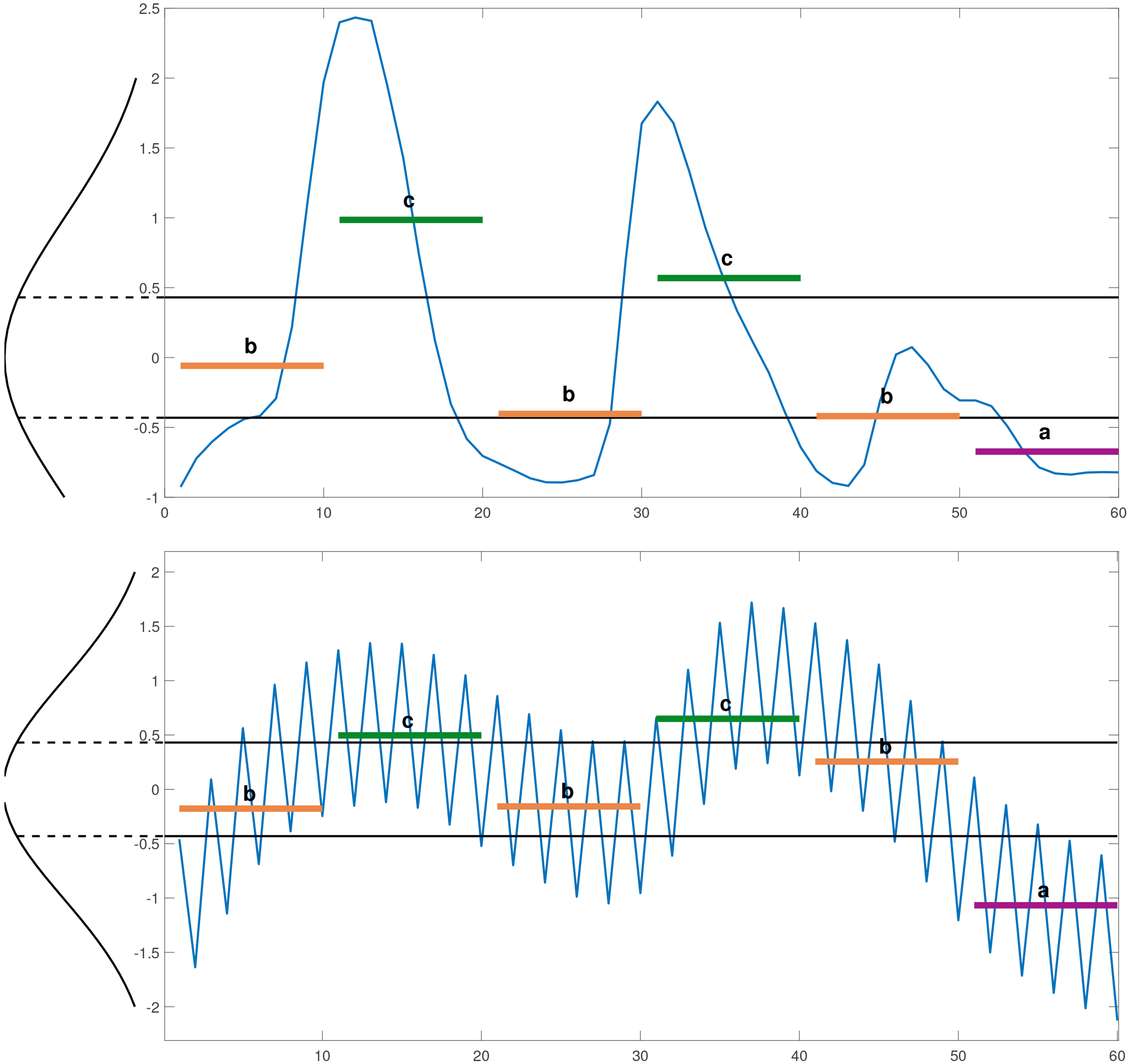

However, the major drawback of SAX representation is that it transforms time series to symbols based on the average values of the segments and ignore important information in the segment. Hence, several different segments having the same average value may be mapped into the same symbol, which is prone to errors in similarity search and classification. Figure 1 shows two very different time series in shape, trend and complexity invariance, but have same SAX representation “bcbcba”. In order to overcome this drawback, some improvements of SAX have been proposed [13, 14, 15].

Extended SAX (ESAX) [13] improves SAX by using additional two discrete points, e.g., maximum and minimum points, besides the average value of a segment. SAX_TD [14] overcomes the drawback of SAX based on a trend distance using the starting and the ending points of segments. Then, the original SAX distance is integrated with weighted trend distance to form the SAX_TD’s distance measure. Alternatively, the improvement based on its statistical features has been proposed in [15], called SAX_SD. Besides storing the symbol of original SAX, SAX_SD uses the standard deviation of the corresponding segment to make more efficient performance.

Recently, complexity invariance has been successfully exploited in time series classification tasks [16]. Intuition tells us that six different time series shown in Fig. 2 are different in complexity invariance (at 0.0951, 0.07231, 0.05866, 0.04836, 0.02364, 0.0093 in the order from left to right and top to bottom), but the same in average values (at 0) and trends; very similar in their starting and ending points; approximate in standard deviation. Hence, the complexity-invariant values may help improving the performance of time series classification and also of time series representation.

Figure 2.

Six time series are different but they have the same average value (at 0).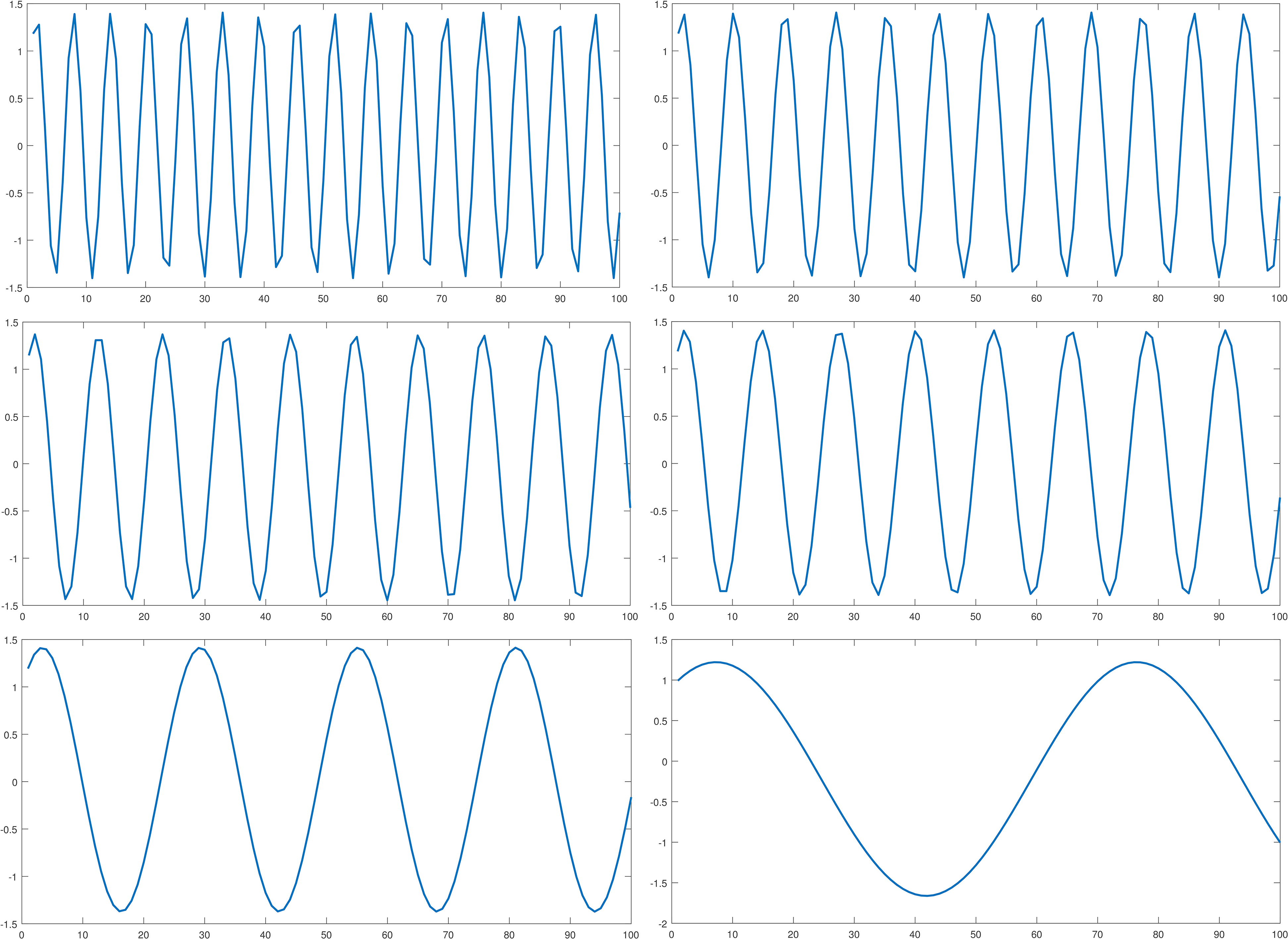

In this work, we proposed a novel representation of time series, called CSAX. Our method represents time series to sequence of original SAX’s alphabetic symbols and the complexity-invariant value. We also create a new distance measure for our representation. Our comprehensive experiments in time series classification demonstrate that CSAX outperforms SAX and its state-of-the-art improvements. It also has dimensionality reduction ratio better than SAX. In other word, the main contributions of our work are as follows: (1) we propose CSAX that improves SAX representation by using complexity invariance, (2) we define a new distance measure based on CSAX, and (3) we conduct experiments to evaluate CSAX and show that it outperforms SAX and its state-of-the-art improvements.

The rest of our paper is organized as follows. Section 2 presents background and related work. Section 3 presents CSAX and new distance measure based on CSAX. Section 4 presents experiments and evaluation. Finally, we draw conclusion in Section 5.

2. Background and related work

2.1 Time series

A time series X is a sequence of real numbers collected at regular intervals over a period: $T=t_{1},t_{2},\ldots,t_{n}$ . The periods of collecting are equals, so they are unimportant. Therefore, we can consider a time series as an $n$ -dimensional instance in a metric space. Figure 3 shows some time series data in ECGFiveDays datasets of UCR Time Series Classification Archive.

Figure 3.

Some time series in ECGFiveDay dataset in UCR Time Series Classification Archive.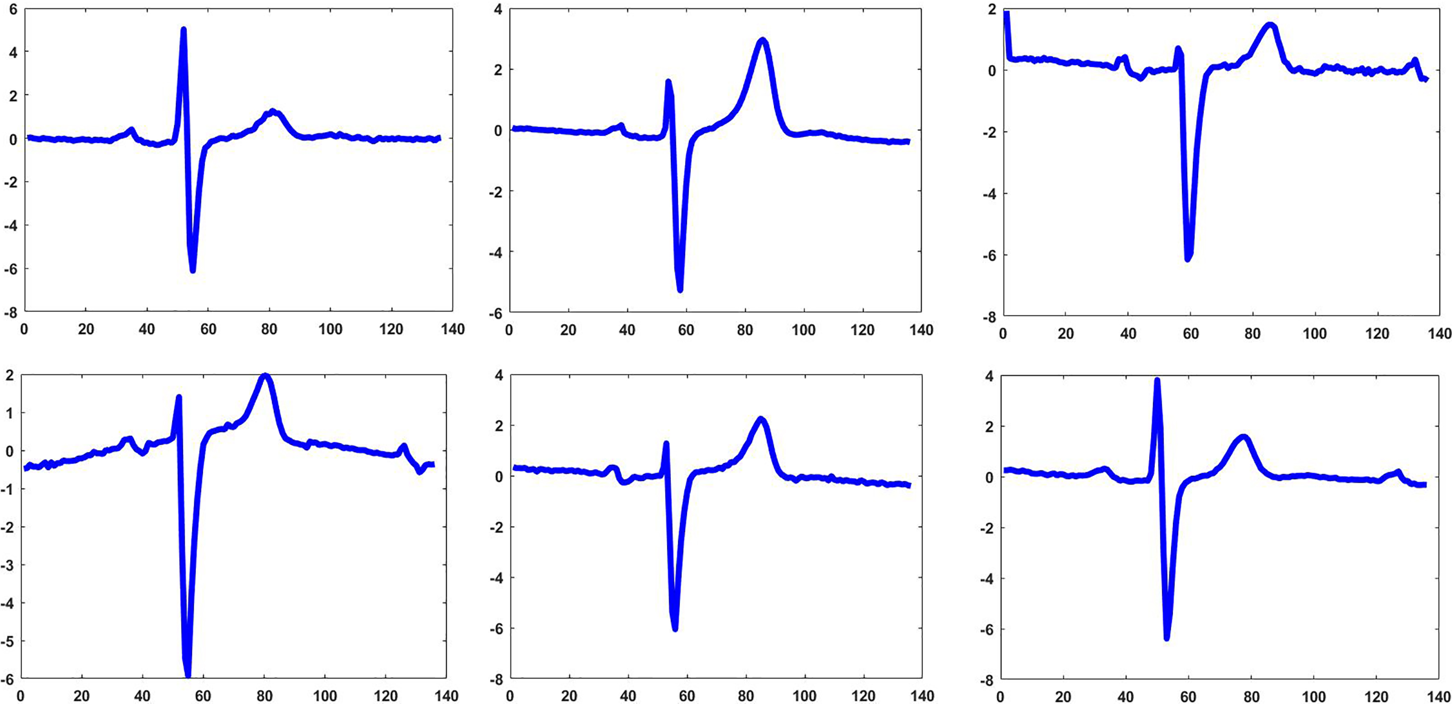

2.2 Symbolic Aggregate approXimation Representation (SAX)

SAX is a most well-known symbolic representation of time series. It transforms the original time series with the length $n$ into a sequence of alphabetic symbols with the length $w$ so that $n\gg w$ . In particular, SAX transforms the original time series into PAA representation and then converts the resulting PAA coefficients into a sequence of symbols in an alphabet. Given a time series $T=t_{1},t_{2},\ldots,t_{n}$ ( $n$ is the length of $T$ ), SAX transforms $T$ into a sequence of $w$ symbols in the alphabet with a size of $\alpha$ by the following steps:

Step 1:
The time series is transformed into Piecewise Aggregate Approximation (PAA) representation [6]. The PAA representation divides the time series $T$ into $w$ equal-sized segments as $\overline{T}=\overline{t_{1}},\overline{t_{2}},\ldots,\overline{t_{w}}$ . Each value of $\overline{T}$ is represented by the average value of each segment and is computed by Eq. (1).

$\displaystyle\overline{t_{i}}=\frac{w}{n}\sum_{j=(n/w)(i-1)+1}^{(n/w)i}t_{j},$ (1)

where $j$ receives values in a range from starting to ending point of each segment.

Table 1
Lookup table for breakpoints, that divide a Gaussian distribution into equal-sized regions, for discrete alphabetic symbol, $\alpha=\overline{3,10}$ (reprinted from Table 3 in [8])

$\alpha=$ 3 $\alpha=$ 4 $\alpha=$ 5 $\alpha=$ 6 $\alpha=$ 7 $\alpha=$ 8 $\alpha=$ 9 $\alpha=$ 10

$\beta_{1}$ $-$ 0.43 $-$ 0.67 $-$ 0.84 $-$ 0.97 $-$ 1.07 $-$ 1.15 $-$ 1.22 $-$ 1.28

$\beta_{2}$ 0.43 0 $-$ 0.25 $-$ 0.43 $-$ 0.57 $-$ 0.68 $-$ 0.77 $-$ 0.84

$\beta_{3}$ 0.67 0.25 0 $-$ 0.18 $-$ 0.32 $-$ 0.43 $-$ 0.52

$\beta_{4}$ 0.84 0.43 0.18 0 $-$ 0.14 $-$ 0.25

$\beta_{5}$ 0.97 0.57 0.32 0.14 0

$\beta_{6}$ 1.07 0.68 0.43 0.25

$\beta_{7}$ 1.15 0.77 0.52

$\beta_{8}$ 1.22 0.84

$\beta_{9}$ 1.28

Figure 4 shows an example of SAX for time series representation.

Figure 4.
An example of SAX Representation for a time series data in Yoga dataset [23] (time series of length 426 is mapped to the sequence of symbols as “eddbbedaaaacdbce”, the segment size, 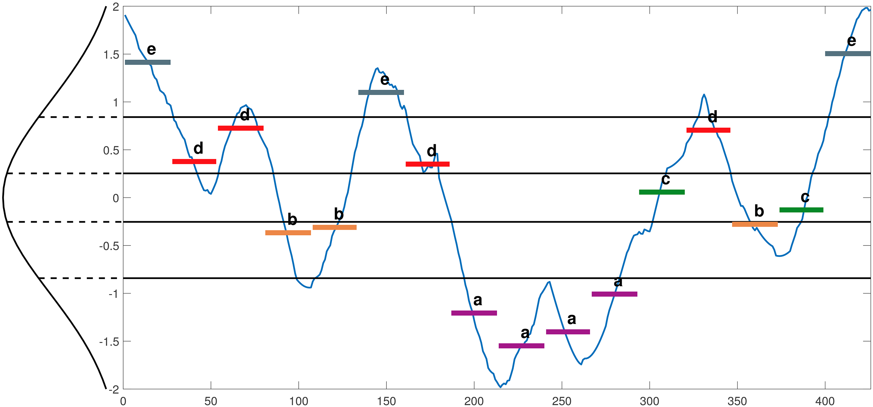$w=$ 16 and the alphabet size, $\alpha=$ 5).

Step 2:
The PAA coefficients are mapped to alphabetic symbols based on the breakpoints $B=\beta_{1},\ldots,\beta_{\alpha-1}$ . Assuming that the time series follows a distribution, those breakpoints divide the distribution space into $\alpha$ equal-sized areas. The lookup table that contains the breakpoints of $\alpha$ from 3 to 10 which is shown in Table 1. For instance, when we use the breakpoints for the alphabet “a, b, c” ( $\alpha=$ 3), we have two breakpoints $\beta_{1}=-$ 0.43 and $\beta_{2}=$ 0.43. And, if a PAA coefficient is lower than $\beta_{1}$ , it is mapped to the symbol “a” and if a PAA coefficient is between $\beta_{1}$ and $\beta_{2}$ , it is mapped to the symbol “b”. Otherwise, it is mapped to the symbol “c”.

2.3 Distance measure for SAX

	$\alpha=$ 3	$\alpha=$ 4	$\alpha=$ 5	$\alpha=$ 6	$\alpha=$ 7	$\alpha=$ 8	$\alpha=$ 9	$\alpha=$ 10
$\beta_{1}$	$-$ 0.43	$-$ 0.67	$-$ 0.84	$-$ 0.97	$-$ 1.07	$-$ 1.15	$-$ 1.22	$-$ 1.28
$\beta_{2}$	0.43	0	$-$ 0.25	$-$ 0.43	$-$ 0.57	$-$ 0.68	$-$ 0.77	$-$ 0.84
$\beta_{3}$		0.67	0.25	0	$-$ 0.18	$-$ 0.32	$-$ 0.43	$-$ 0.52
$\beta_{4}$			0.84	0.43	0.18	0	$-$ 0.14	$-$ 0.25
$\beta_{5}$				0.97	0.57	0.32	0.14	0
$\beta_{6}$					1.07	0.68	0.43	0.25
$\beta_{7}$						1.15	0.77	0.52
$\beta_{8}$							1.22	0.84
$\beta_{9}$								1.28

Given two time series $Q$ and $C$ (length $n$ ), they are transformed into SAX representation $\hat{Q}=\hat{q_{1}},\ldots,\hat{q_{w}}$ and $\hat{C}=\hat{c_{1}},\ldots,\hat{c_{w}}$ with the segment size $w$ . The MINDIST distance for $\hat{Q}$ and $\hat{C}$ is defined as Eq. (2).

$\displaystyle\textit{MINDIST}(\hat{Q},\hat{C})=\sqrt{\frac{n}{w}}\sqrt{\sum_{i% =1}^{w}\textit{dist}(\hat{q_{i}},\hat{c_{i}})^{2}}$ (2)

where $\textit{dist}()$ function is implemented by using Table 1 and calculated by using Eq. (3).

$\displaystyle\textit{dist}(\hat{q},\hat{c})=\left\{\begin{array}[]{ll}0,&% \textit{if }|\hat{q}-\hat{c}|\leqslant 1\\ \beta_{\max(\hat{q},\hat{c})-1}-\beta_{\min(\hat{q},\hat{c})},&\textit{% otherwise}\\ \end{array}\right.$ (3)

Table 2 shows the sample of lookup table for MINDIST function.

Table 2

The sample of lookup table for MINDIST function with alphabet size $\alpha=$ 5 (extended from Table 4 alphabet size $\alpha=$ 4 in [8])

	a	b	c	d	e
a	0	0	0.59	1.09	1.68
b	0	0	0	0.5	1.09
c	0.59	0	0	0	0.59
d	1.09	0.5	0	0	0
e	1.68	1.09	0.59	0	0

In the case of real-valued time series, Euclidean distance is one of the most well-known methods. Given two time series $Q=q_{1},\ldots,q_{n}$ and $C=c_{1},\ldots,c_{n}$ , Euclidean distance between $Q$ and $C$ is calculated using Eq. (4).

$\displaystyle ED(Q,C)=\sqrt{\sum_{i=1}^{n}(q_{i}-c_{i})^{2}}$ (4)

2.4 Improvements of SAX

SAX just uses the average values to represent the time series. Hence, it ignores some important information. This drawback causes errors in classification and other data mining tasks for time series. In this section, we introduce improvements of SAX in time series classification.

In [18], Hugueney introduced a method that uses Adaptive Piecewise Constant Approximation (APCA) [7] in place of PAA [6] in original SAX. In [19], Marwan et al. proposed Genetic Algorithm SAX (GASAX) to determine breakpoints based on Genetic Algorithm (GA) [20]. The authors argued that Gaussianity’s assumption oversimplifies the problem of SAX representation and may result in high values of error when performing time-series mining tasks. The objective of GA is to find the configuration that provides the best value of a fitness function [19]. The configuration means the optimal or nearly optimal solution for the problem. It has the following elements: a individual’s population, selection according to fitness, crossover to produce new offspring, and random mutation of new offspring. Although GASAX works well on both normalized and non-normalized time series data, GA needs to determine the appropriate control parameters for its elements and it is important to keep a balance between elements to obtain an optimal solution.

Then, Extended SAX method (ESAX) is proposed by Lkhagva [13]. This representations improved original SAX by adding two new points (min and max points) besides the average values in each equal-sized segments. After that, those points are transformed into alphabetic symbols by the same way of SAX. ESAX has been demonstrated to be effective for financial time series data. However, the storage space of ESAX is triple times than that of SAX representation and the execution time of ESAX is significantly higher than the original SAX.

In 2015, Yin et al. proposed a method called Trend Feature Symbolic Approximation (TFSA) [21]. It uses a two-step segmentation technique to segment long time series data rapidly. TFSA proved that it guarantees the lower bounding distance, better segmentation, and classification accuracy. In 2013 and 2014, there are two methods that improve the original SAX by using trend feature of time series: 1d-SAX [17] of Malinowski et al. and SAX-TD [14] of Youqiang et al. The trend feature in 1d-SAX is calculated by using the quantization of linear regression on each segment. That is why the method called 1d-SAX [17]. SAX_TD uses the value of starting point and ending point to determine the trend feature of each segment. The experimental results in [14] show that SAX_TD outperforms the original SAX and ESAX.

SAX_SD is other improvement of SAX [15]. It is proposed by Zan et al. It improve the SAX by using the standard deviation values and average values to represent the time series. The authors in [15] indicated that SAX_SD outperforms the original SAX, ESAX and SAX_TD.

The original SAX has been improved in various different aspects in different tasks. However, the complexity invariance of time series is still not exploited. Figure 2 shows the major limitation of the original SAX and its improvements. Hence, in order to overcome this drawback, we propose a novel improvement of SAX.

2.5 Complexity invariance measure for time series

It was first proposed by Yan et al. [22] and was used by Batista and Keogh [16] for enhance the accuracy of their novel distance measure, called Complexity-invariant Distance. It is based on the fact that complex time series are commonly considered more similar to simple time series than to other complex time series they look like. For instance, in Fig. 2, we have six time series with the same in average value (at 0), the same trend, very similar in their starting and ending points, and approximate in standard deviation. The only different between those time series is the complex of them. In [16] the time series’ complexity invariance is calculated by Eq. (5)

$\displaystyle CE(S)=\sqrt{\sum_{i=1}^{v-1}(s_{i+1}-s_{i})^{2}}$ (5)

3. The proposed time series representation

3.1 CSAX: Complexity-invariant SAX

This section presents a novel representation for time series. It is an improvement of SAX representation by using complexity invariance, namely CSAX. In particular, given a time series, our method provides an additional complexity-invariant feature besides the average feature of SAX representation. The complexity invariance that we use in CSAX is a significant important feature to determine difference in shape of time series. As shown in Fig. 2, six different time series are the same in average value; similar in values of starting and ending points (the features which SAX_TD exploit); similar in maximum and minimum points (two new additional points in ESAX), respectively; the same in up and down trend; and the same standard deviation value (SAX_SD uses the standard deviation as an additional feature). However, those time series in Fig. 2 are different in the complexity-invariant values: 0.0951, 0.07231, 0.05866, 0.04836, 0.02364, 0.0093, decreasing from the first time series to sixth time series, respectively. It means that the complexity invariance can help to fix the limitation of the original SAX representation and its improvements.

Our method transforms the time series to a sequence of alphabetic symbols in an alphabet based on the original SAX. Then, it calculates complexity-invariant value of each segment corresponding to a symbol in the sequence. In particular, given a segment of a time series $S=s_{1},\ldots,s_{v}$ of length $v$ , the complexity-invariant value of this segment is calculated using Eq. (6), where we use the denominator $v-1$ to reduce the overwhelming influence of complexity-invariant feature in the distance measure. After this step, the original time series is transformed into a sequence of symbols in combination with complexity-invariant values so that one symbol corresponds to a complexity-invariant value of the segment from which the symbol is inferred. For instance, the time series in Fig. 4 is represented as “ $(e,0.0081)$ , $(d,0.0089)$ , $(d,0.0098)$ , $(b,0.0130)$ , $(b,0.0128)$ , $(e,0.0110)$ , $(d,0.0155)$ , $(a,0.0137)$ , $(a,0.0097)$ , $(a,0.0089)$ , $(a,0.0102)$ , $(c,0.0089)$ , $(d,0.0115)$ , $(b,0.0071)$ , $(c,0.0114)$ , $(e,0.0112)$ ”, in which the numbers are complexity-invariant values.

$\displaystyle C(S)=\frac{1}{v-1}CE(S)$ (6)

where $CE(S)$ is calculated by Eq. (5).

3.2 Distance measure for CSAX

A novel distance measure for CSAX is defined based on the sequence of symbols and their corresponding complexity-invariant values. Given two time series $Q$ and $C$ of length $n$ , after transforming these time series into sequences of symbols and calculating complexity-invariant values, we have the transformed time series $\hat{Q}=(\hat{q_{1}},\textit{ciq}_{1}),\ldots,(\hat{q_{w}},\textit{ciq}_{w})$ and $\hat{C}=(\hat{c_{1}},\textit{cic}_{1}),\ldots,(\hat{c_{w}},\textit{cic}_{w})$ , where $w$ is the segment size and $\textit{ciq}_{1},\ldots,\textit{ciq}_{w},\textit{cic}_{1},\ldots,\textit{cic}_% {w}$ is calculated by Eq. (6). The distance between these two time series based on the complexity invariance is calculated using Eq. (7).

$\displaystyle\textit{CSAX}(\hat{Q},\hat{C})=\sqrt{\frac{n}{w}}\sqrt{\sum_{i=1}% ^{w}(\textit{dist}(\hat{q_{i}},\hat{c_{i}})+(\textit{ciq}_{i}-\textit{cic}_{i}% )^{2})}$ (7)

where $\textit{dist}(\hat{q_{i}},\hat{c_{i}})$ is calculated in the same way with SAX representation using Eq. (3).

In the term of dimensionality reduction, the time series of length $n$ is reduced by ratio $w/n$ . And, the segment size $w$ has the significant influence not only on dimensionality reduction but also on the appearance of complexity-invariant feature. The smaller $w$ , the longer segment; hence, this inflects the appearance of complexity-invariant feature (make it larger). In the other hand, the lager $w$ , the smaller complexity-invariant value. Given two time series (in Gun-Point dataset [23], first one is 19th time series in TRAIN file and second one is 24th time series in TEST file), whose length is 150 and Euclidean distance is 7.4182, with alphabet size $\alpha=$ 5, Table 3 shows the distances of the original SAX and CSAX corresponding to different values of the segment size. Each column of the table shows the value of $w$ , the distance between these two time series based on SAX, and the distance between these two time series using CSAX, respectively. Based on the resulting distances, one can figure out that CSAX is closer with the true distance (Euclidean distance) than that of original SAX.

Table 3

SAX-CID and SAX distance with different values of $w$ parameter. The Euclidean distance is 7.4182

$w$	2	4	8	16	32	64
SAX	0	2.1941	3.6024	3.6942	3.8298	3.9608
CSAX	0.0130	2.2130	3.6901	3.7965	4.1005	4.3315

Table 4

Description of 20 datasets in UCR Time Series Classification Archive [23]

No.	Dataset	Number of classes	Size of training set	Size of testing set	Time series length	Type
1	Synthetic Control	6	300	300	60	Simulated
2	Gun Point	2	50	150	150	Motion
3	CBF	3	30	900	128	Simulated
4	FaceAll	14	560	1690	131	Image
5	OSULeaf	6	200	242	427	Image
6	SwedishLeaf	15	500	625	128	Image
7	50words	50	450	455	270	Image
8	Trace	4	100	100	275	Sensor
9	Two Patterns	4	1000	4000	128	Simulated
10	Wafer	2	1000	6174	152	Sensor
11	FaceFour	4	24	88	350	Image
12	Lighting2	2	60	61	637	Sensor
13	Lighting7	7	70	73	319	Sensor
14	ECG200	2	100	100	96	ECG
15	Adiac	37	390	391	176	Image
16	Yoga	2	300	3000	426	Image
17	Fish	7	175	175	463	Image
18	Beef	7	105	105	144	Spectro
19	Coffee	4	60	60	577	Spectro
20	OliveOil	5	30	30	470	Spectro

4. Experimental evaluation

In this section, we present experiments to evaluate CSAX. Firstly, we introduce the used datasets, comparison methods, and parameter settings. Then we compare the experimental results of our proposed CSAX with those of Euclidean distance, the original SAX, ESAX, SAX_TD and SAX_SD in the terms of classification error rate, dimensionality reduction and efficiency. We implemented methods in Matlab R2016a and conducted the experiments on an Intel(R) Core(TM) i7-4700MQ CPU @ 2.40 GHz, 16 GB RAM, Lenovo y510p Laptop.

4.1 Datasets

We use first 20 datasets in UCR Time Series Classification Archive [23] in order to compare with the previous methods that were evaluated on the same datasets. Each dataset is divided into a training set and a testing set. Table 4 shows the brief description of each dataset: name, number of classes, size of training and testing set, length of the time series and its type.

4.2 Comparison methods and parameter settings

We deploy the same comparison method used in [14, 15] for evaluation. In particular, we compare the experimental results of our proposed CSAX with those of Euclidean distance, the original SAX, and three other improvements of SAX: ESAX, SAX_TD and SAX_SD. The reason to choose these three improvements is that distance measures for these representations have been modified as well. Because 1-Nearest Neighbor (1-NN) classifier directly reflects the performance of the distance measures, we use this classifier to compare their classification accuracy. For Euclidean distance, we do not need to set any parameter because it is a parameter-free distance. For other distances, i.e., SAX, ESAX, SAX_TD and SAX_SD, two parameters that are $w$ (segment size) and $\alpha$ (alphabet size) decide their classification accuracy. Therefore, it is neccessary to find the best optimal values of the segment size and alphabet size to achieve the best classification accuracy.

Given time series of length $n$ , two parameters $w$ and $\alpha$ are picked by using the following criteria (and the same paradigm as applied in [13] for fairness of comparison):

1.
Searching the value of $w$ from 2 up to $n/2$ (double the $w$ value each time).
2.
Searching the value for $\alpha$ from 3 to 10.
3.
Choosing the smaller set of parameters (priority $w$ value) if two sets of parameter setting have the same classification accuracy.

For the dimensionality reduction ratio, we measure this ratio using Eq. (8) [14].

$\displaystyle\textit{Dimensionality Reduction Ratio}=\frac{\textit{Number Of % Reduced Data}}{\textit{Number Of Original Data}}$ (8)

Table 5
Reduction ratio and space complexity of each representation in comparison

Name Reduction ratio Space complexity

SAX $w/n$ $w(\log_{2}(\alpha))/n$

ESAX $3w/n$ $3w(\log_{2}(\alpha))/n$

SAX_TD $(2w+1)/n$ $w(\log_{2}(\alpha)+r)/n+r$

SAX_SD $2w/n$ $w(\log_{2}(\alpha)+r)/n$

CSAX $2w/n$ $w(\log_{2}(\alpha)+r)/n$

Based on Eq. (8), we show the dimensionality reduction ratio and the space complexity of each comparison method in Table 5 where $w$ is the segment size and $n$ is the length of the original time series. In Table 5, $\log_{2}(\alpha)$ is the number of bits to store symbols in the alphabet, and $r$ is a number of bits to represent a real number.
4.3 Classification accuracy comparison

Name	Reduction ratio	Space complexity
SAX	$w/n$	$w(\log_{2}(\alpha))/n$
ESAX	$3w/n$	$3w(\log_{2}(\alpha))/n$
SAX_TD	$(2w+1)/n$	$w(\log_{2}(\alpha)+r)/n+r$
SAX_SD	$2w/n$	$w(\log_{2}(\alpha)+r)/n$
CSAX	$2w/n$	$w(\log_{2}(\alpha)+r)/n$

Table 6
The sign test results of CSAX vs. other methods. A $p$ -value less than or equal to 0.05 indicates a significant improvement

Method	$n_{+}$	$n_{0}$	$n_{-}$	$p$ -value
CSAX vs Euclidean distance	18	1	1	$p<$ 0.01
CSAX vs SAX	16	2	2	$p<$ 0.01
CSAX vs ESAX	18	1	1	$p<$ 0.01
CSAX vs SAX_TD	14	4	2	$p<$ 0.01
CSAX vs SAX_SD	12	4	4	0.01 $<p<$ 0.05

Table 7

1-NN classification error rate of Euclidean distance, the best error rate of 1-NN classification, the best set of $w$ , $\alpha$ of SAX, ESAX, SAX_TD, SAX_SD, and proposed CSAX on 20 data sets (describing in Fig. 4)

Dataset no.	Euclidean distance error	1-NN error	w	a	1-NN error	w	a	1-NN error	w	a	1-NN error	w	a	1-NN error	w	a
		SAX			ESAX			SAX_TD			SAX_SD			CSAX
1	0.120	0.017	16	10	0.003	16	10	0.050	16	10	0.033	16	10	0.023	4	7
2	0.087	0.193	64	10	0.213	64	10	0.470	4	3	0.033	32	3	0.027	4	7
3	0.148	0.102	32	10	0.090	64	10	0.088	4	10	0.020	4	10	0.042	8	6
4	0.286	0.331	64	10	0.315	64	9	0.201	16	8	0.200	64	3	0.176	16	3
5	0.479	0.463	128	10	0.467	16	9	0.438	32	7	0.433	32	3	0.397	16	3
6	0.211	0.491	32	10	0.413	64	10	0.211	16	7	0.134	32	3	0.102	16	5
7	0.369	0.345	128	10	0.354	32	10	0.358	64	10	0.325	8	9	0.323	16	3
8	0.240	0.460	128	10	0.330	4	10	0.230	32	7	0.060	8	7	0.000	4	3
9	0.093	0.082	32	10	0.134	64	10	0.071	16	10	0.091	8	10	0.062	16	9
10	0.005	0.003	64	10	0.003	64	9	0.004	64	7	0.013	4	9	0.003	32	6
11	0.216	0.159	128	10	0.193	128	7	0.159	32	9	0.114	16	7	0.159	64	10
12	0.246	0.213	256	10	0.262	32	7	0.197	32	7	0.164	4	10	0.164	64	9
13	0.425	0.384	128	10	0.370	128	8	0.301	8	10	0.370	4	10	0.288	16	6
14	0.120	0.102	32	10	0.130	32	10	0.090	32	7	0.070	4	9	0.110	16	6
15	0.389	0.890	64	10	0.890	64	10	0.284	16	8	0.284	16	5	0.263	32	7
16	0.170	0.193	128	10	0.201	128	10	0.169	128	3	0.162	15	10	0.181	32	3
17	0.217	0.480	128	10	0.469	128	10	0.189	64	9	0.189	64	9	0.149	64	9
18	0.333	0.567	128	10	0.533	32	9	0.300	64	9	0.300	16	9	0.300	64	9
19	0.000	0.464	128	10	0.464	4	5	0.000	16	3	0.000	8	3	0.000	4	3
20	0.133	0.833	256	10	0.833	2	3	0.130	64	3	0.133	128	3	0.130	32	3
Average	0.214	0.339			0.333			0.197			0.156			0.145

Figure 5.

Classification error rate of compared methods with different values of parameters 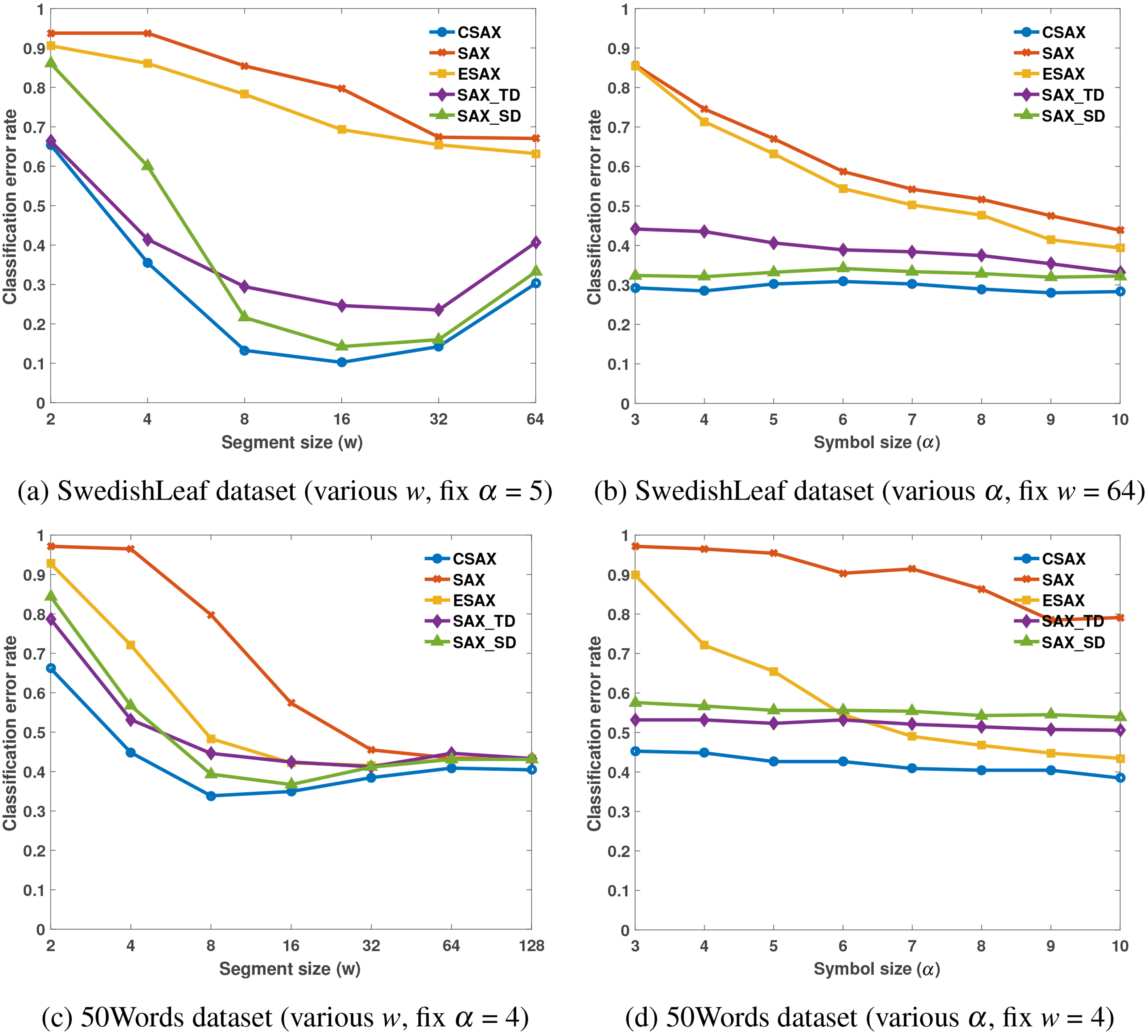$w$ and $\alpha$ .

Figure 6.

The scatter charts indicate the pairwise of error rates of our proposed CSAX and Euclidean distance, distances of SAX, ESAX, SAX_TD, SAX_SD on 20 datasets in UCR Time Series Classification Archive. In the lower triangle, the square points illustrate the datasets in which our CSAX is more accuracy than other methods. In Upper triangle, the round points illustrate the datasets in which other methods are more accuracy than CSAX. In diagonal line, the triangle points illustrate the datasets in which our CSAX and other methods have same accuracy.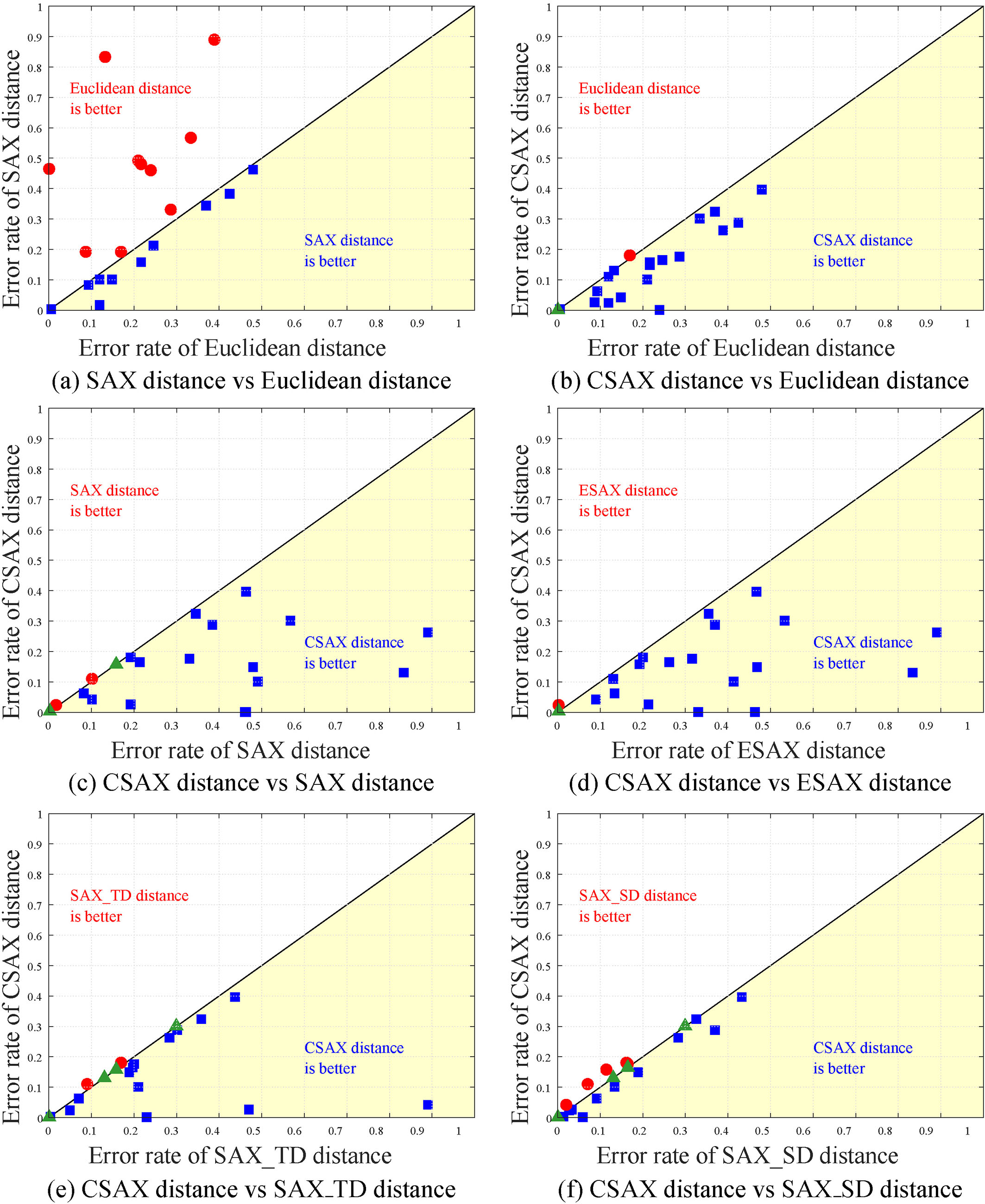

Figure 7.

The running time of five compared methods with different values of the parameter 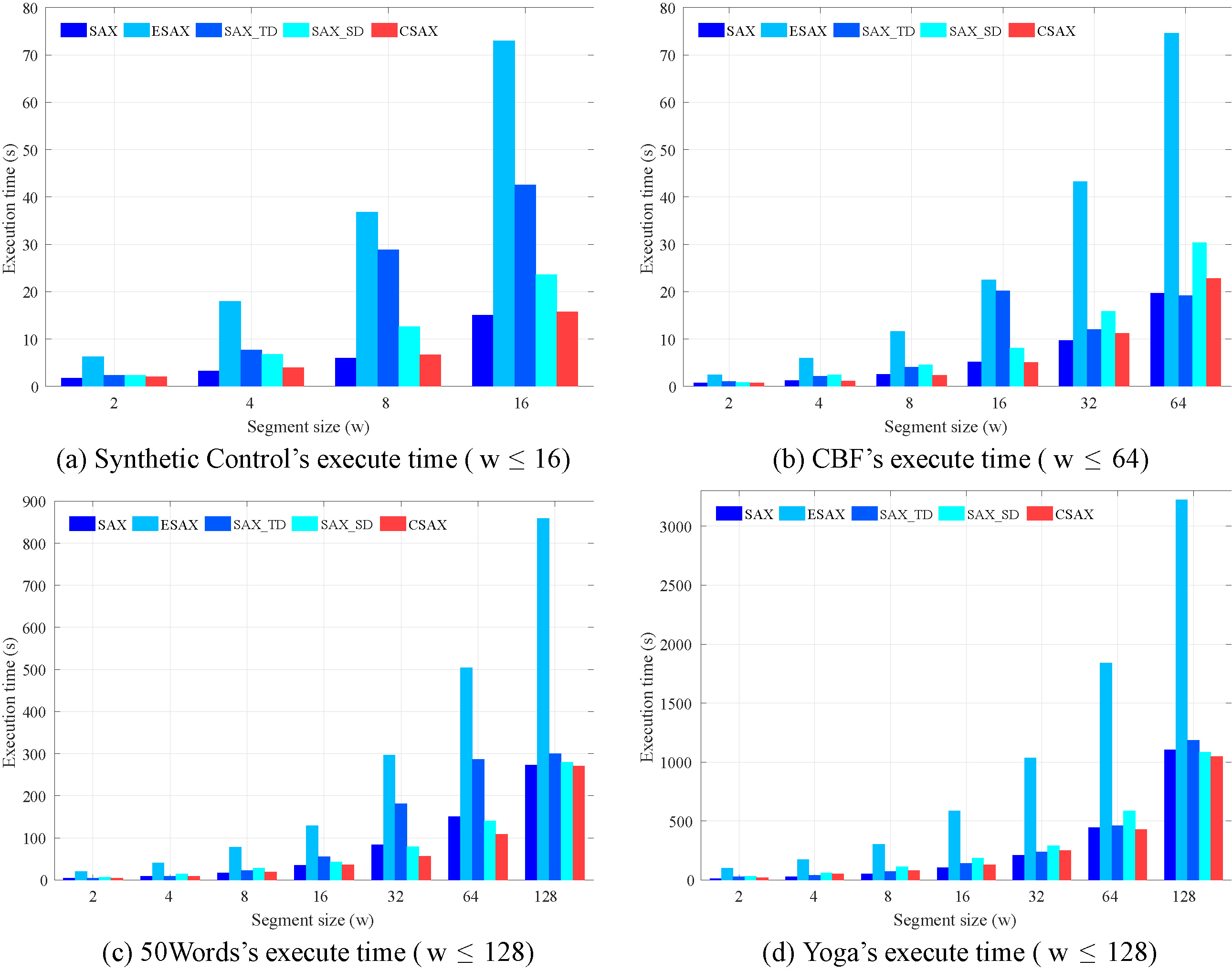$w$ and $\alpha$ is fixed at 10. (a) Synthesis Control dataset ( $w\leqslant$ 16), (b) CBF dataset ( $w\leqslant$ 64), (c) 50Words dataset ( $w\leqslant$ 128) and (d) Yoga dataset ( $w\leqslant$ 128).

Table 8

The dimensional reduction ratio of SAX, ESAX, SAX_TD, SAX_SD, and proposed CSAX

Dataset	SAX ratio	ESAX ratio	SAX_TD ratio	SAX_SD ratio	CSAX ratio
1	0.267	0.800	0.550	0.533	0.133
2	0.427	1.280	0.060	0.427	0.053
3	0.250	1.500	0.070	0.063	0.125
4	0.489	1.466	0.252	0.977	0.244
5	0.300	0.112	0.152	0.150	0.075
6	0.250	1.500	0.258	0.500	0.250
7	0.474	0.356	0.478	0.059	0.119
8	0.465	0.044	0.236	0.058	0.029
9	0.250	1.500	0.258	0.125	0.250
10	0.421	1.263	0.849	0.053	0.421
11	0.366	1.097	0.186	0.091	0.366
12	0.402	0.151	0.102	0.013	0.201
13	0.401	1.204	0.053	0.025	0.100
14	0.344	1.032	0.699	0.086	0.344
15	0.364	1.091	0.188	0.182	0.364
16	0.300	0.901	0.603	0.075	0.150
17	0.276	0.829	0.279	0.276	0.276
18	0.272	0.204	0.274	0.068	0.272
19	0.448	0.042	0.115	0.056	0.028
20	0.449	0.011	0.226	0.449	0.112
Average	0.361	0.819	0.294	0.213	0.196

Table 6 shows the overall results of 1-NN classification in 20 datasets represented in Table 4. In which, we highlight the lowest classification error rates for each distance measure. The proposed CSAX has the lowest error rate in most of datasets (15/20). SAX_SD has the lowest error rate in 7/20 datasets, followed by SAX_TD and ESAX with 2/20 datasets. Finally, the original SAX and Euclidean have the lowest error rate in just 1/20 dataset. In Table 7, $n_{+}$ , $n_{-}$ , and $n_{0}$ denote the number of datasets where error rates of CSAX are better than, worse than and equal to those of other methods, respectively, on the same datasets. Experimental results shown in Tables 6 and 7 indicate that CSAX has the lowest average error rate at 0.145 and outperforms Euclidean distance, SAX, ESAX, SAX_TD, and SAX_SD in most of datasets. CSAX gives accuracy better in 18/20, 16/20, 18/20, 14/20 and 12/20 datasets, worse in 1/20, 2/20, 1/20, 2/20 and 4/20 datasets, and the same in 1/20, 2/20, 1/20, 4/20 and 4/20 datasets with Euclidean distance, SAX, ESAX, SAX_TD, and SAX_SD, respectively.

In Fig. 5, we provide four line charts to compare CSAX with SAX, ESAX, SAX_TD, and SAX_SD using different parameters $w$ and $\alpha$ in SwedishLeaf and 50Words datasets. In particular, on SwedishLeaf dataset, the setting for the pair ( $w$ , $\alpha$ ) are ( $w$ , 5) in Fig. 5a and (64, $\alpha$ ) in Fig. 5b; on 50Words dataset, the setting for the pair ( $w$ , $\alpha$ ) are ( $w$ , 4) in Fig. 5c and (4, $\alpha$ ) in Fig. 5d. In overall, CSAX gives the lowest error rates in all experimental settings, accordingly. It shows that our proposed CSAX outperforms other methods with different values of parameters $w$ and $\alpha$ used in the experiments.

We provide six scatter charts for illustrating the performance of pairwise distance measures in Fig. 6. In those charts, error rates of two compared methods are used as the $O x$ and $O y$ coordinates of a point which represents experimental datasets. The region with more points corresponding a method shows that the method is better than another. In Fig. 6, we first compare the Euclidean distance with SAX distance in Fig. 6a. The number of data point in Euclidean distance region is not only higher than that of SAX distance region, but also there are some data points in that the error rate of Euclidean distance is significantly smaller than that of SAX distance (SAX distance has a very bad result in Adiac and OliveOil datasets at 0.89 and 0.833, respectively).

In Fig. 6b–f, we compare our proposed CSAX with Euclidean distance, SAX, ESAX, SAX_TD, and SAX_SD, respectively. In general, our proposed CSAX outperforms other methods in the number of data points in its region and the distances of these points from the diagonal line. Especially, in Trace and Fish datasets, CSAX has the error rate at 0 and 0.149, respectively, while the lowest error rate of other methods at 0.06 (the error rate of SAX_SD) and 0.189 (the error rate of both SAX_TD and SAX_SD), respectively.

4.4 Comparison of dimensionality reduction and computation time

We provide the comparison of the running time, with various $w$ , of CSAX and SAX, ESAX, SAX_TD, SAX_SD on Synthesis Control, CBF, 50Words and Yoga datasets in Fig. 7. We fix the parameter $\alpha$ at maximum value ( $\alpha=$ 10)2

²
Since the difference in computation time is mainly determined by the value of parameter w, we fix the value of $\alpha$ .

and maximum

w

at 16, 64, 128 and 128, respectively (because of different length of time series in four datasets). The results are presented in Fig. 7. Note that, the running time consists of the transformation time (using representation method) and classification time (using the classification method).

Figure 8.

Dimensionality reduction ratios of the SAX, the ESAX, the SAX_TD, the SAX_SD, and CSAX on 20 data sets with their smallest error rates.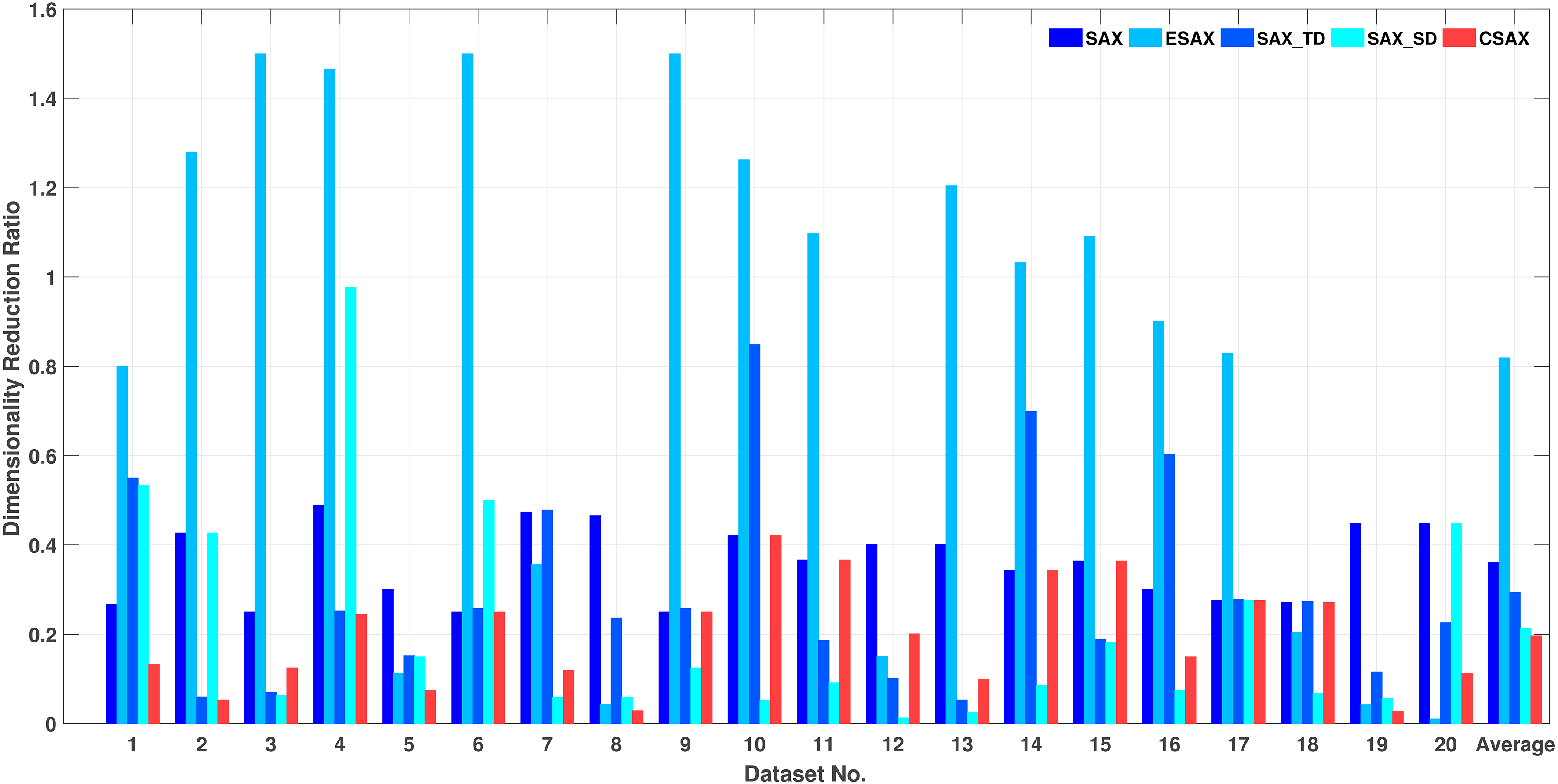

Overall, the running time of CSAX is similar to the original SAX and lower than those of ESAX, SAX_TD and SAX_SD in most of different $w$ size in all four datasets. For example, on Yoga dataset, CSAX takes 1047 seconds while SAX, ESAX, SAX_TD, SAX_SD take 1105, 3223, 1185 and 1114 seconds, respectively.

Finally, SAX is very well-known for dimensionality reduction with the ratio ( $w/n$ ). The results of dimensionality reduction ratio of SAX, ESAX, SAX_TD, SAX_SD and the proposed CSAX with the lowest error rate is presented in Table 8 and is demontrated in Fig. 8. The experimental results show that CSAX has the dimensionality reduction ratio better than those of other methods with the average ratio at 0.196 while the average ratios of SAX, ESAX, SAX_TD and SAX_SD are 0.361, 0.819, 0.294 and 0.213, respectively. Especially, in Synthesis Control dataset, the dimensionality reduction ratio of CSAX is at 0.133 while the ratios of other methods are 0.267, 0.8, 0.55 and 0.533, respectively. As a result, CSAX outperforms the other compared methods not only in term of classification performance, but also in the term of dimensionality reduction ratio.

5. Conclusion

In this paper, we first summarize the background knowledge of SAX representation and its most well-known improvements. Then, we point out the drawback of SAX and propose a novel improvement of SAX representation, called CSAX. CSAX uses the complexity-invariant values of segments of the original time series as additional features besides the average values used in the original SAX. The experimental results demonstrate that CSAX outperforms SAX and its three well-known improvements, i.e., ESAX, SAX_TD and SAX_SD, in 20 dataset of UCR Time Series Classification Archives in the terms of classification accuracy and dimensionality reduction ratio. In addition, CSAX also achieves computational efficiency better than that of ESAX, SAX_TD, and SAX_SD.

We have gradually entered into a new era of Internet of Things (IoT), where billions of connected devices constantly produce a tremendous amount of streaming time series in a period of time. One can first apply CSAX to transform each time series into an alphabetic string, then adapt language model pre-training such as word2vec [26] or Transformer [25] in the field of natural language processing or the embedding of DNA reads [27] in the field of computational biology to learn distributed representations of the obtained alphabetic strings in the unsupervised setting. After that, the pre-trained models are exploited to extract features or fine-tune for downstream tasks such as classification, clustering, or search of time series. In [24], the authors initially prove that the distributed representation of time series, namely Singnal2vec, trained by using Skip-gram model [26] outperforms SAX and PAA. We put these lines of research in future.

References

Agrawal

Faloutsos

and Swami

A.N.

, Efficient Similarity Search in Sequence Databases, in: Proceedings of the 4th International Conference on Foundations of Data Organization and Algorithms (FODO ’93), 1993, pp. 69–84.

Faloutsos

Ranganathan

and Manolopoulos

, Fast Subsequence Matching in Time-series Databases, in: Proceedings of the 1994 ACM SIGMOD International Conference on Management of Data (SIGMOD ’94), 1994, pp. 419–429.

Kin-Pong

and Ada

W.F.

, Efficient time series matching by wavelets, in: Proceedings 15th International Conference on Data Engineering (Cat. No.99CB36337), 1999, pp. 126–133.

Korn

Jagadish

H.V.

and Faloutsos

, Efficiently Supporting Ad Hoc Queries in Large Datasets of Time Sequences, in: Proceedings of the 1997 ACM SIGMOD International Conference on Management of Data (SIGMOD ’97), 1997, pp. 289–300.

Ravi Kanth

K.V.

Agrawal

and Singh

, Dimensionality Reduction for Similarity Searching in Dynamic Databases, in: Proceedings of the 1998 ACM SIGMOD International Conference on Management of Data (SIGMOD ’98), 1998, pp. 166–176.

Keogh

Chakrabarti

Pazzani

and Mehrotra

, Dimensionality reduction for fast similarity search in large time series databases, Knowledge and Information Systems 3(3) (2001), 263–286.

Chakrabarti

Keogh

Mehrotra

and Pazzani

, Locally adaptive dimensionality reduction for indexing large time series databases, ACM Trans. Database Syst. 27(2) (2002), 188–228.

Lin

Keogh

Wei

and Lonardi

, Experiencing SAX: A novel symbolic representation of time series, Data Min. Knowl. Discov. 2(2) (2007), 107–144.

Song

Wang

Zhang

and Fan

, Empirical study of symbolic aggregate approximation for time series classification, Intelligent Data Analysis 21(1) (2017), 135–150.

10.

Rakthanmanon

and Keogh

, Fast Shapelets: A Scalable Algorithm for Discovering Time Series Shapelets, in: Proceedings of the 2013 SIAM International Conference on Data Mining, 2003, pp. 668–676.

11.

Barnaghi

Ganz

Henson

and Sheth

, Computing perception from sensor data, in: 2012 IEEE Sensors, 2012, pp. 1–4.

12.

Tayebi

Krishnaswamy

Waluyo

A.B.

Sinha

and Gaber

M.M.

, RA-SAX: Resource-Aware Symbolic Aggregate Approximation for Mobile ECG Analysis, in: 2011 IEEE 12th International Conference on Mobile Data Management, 2011, pp. 289–290.

13.

Lkhagva

Suzuki

and Kawagoe

, New Time Series Data Representation ESAX for Financial Applications, in: 22nd International Conference on Data Engineering Workshops (ICDEW’06), 2006, pp. x115–x115.

14.

Youqiang

Jiuyong

Jixue

Bingyu

and Christopher

, An improvement of symbolic aggregate approximation distance measure for time series, Neurocomputing 138(Supplement C) (2014), 189–198.

15.

Zan

and Yamana

, An Improved Symbolic Aggregate Approximation Distance Measure Based on Its Statistical Features, in: Proceedings of the 18th International Conference on Information Integration and Web-based Applications and Services (iiWAS ’16), 2016, pp. 72–80.

16.

Batista

G.E.A.P.A.

Keogh

Tataw

O.M.

and Vinicius

D.S.

, CID: An efficient complexity-invariant distance for time series, Data Mining and Knowledge Discovery 28(3) (2014), 634–669.

17.

Malinowski

Guyet

Quiniou

and Tavenard

, 1d-SAX: A Novel Symbolic Representation for Time Series, in: Advances in Intelligent Data Analysis XII: 12th International Symposium (IDA 2013), 2013, pp. 273–284.

18.

Hugueney

, Adaptive Segmentation-Based Symbolic Representations of Time Series for Better Modeling and Lower Bounding Distance Measures, in: Knowledge Discovery in Databases (PKDD 2006), 2006, pp. 545–552.

19.

Fuad

and Marwan

, Genetic Algorithms-Based Symbolic Aggregate Approximation, in: The 14th Int’l Conf. on Data Warehousing and Knowledge Discovery, 2012, pp. 105–116.

20.

Mitchell

, An Introduction to Genetic Algorithms, MIT Press, Cambridge MA, 1998.

21.

Yin

Yang

Zhu

and Zhang

, Symbolic representation based on trend features for knowledge discovery in long time series, in: Frontiers of Information Technology and Electronic Engineering, 2015, pp. 744–758.

22.

Yan

Fang

and Ma

, An approach of time series piecewise linear representation based on local maximum minimum and extremum, Journal of Information and Computational Science (2013), 2747–2756.

23.

Chen

Keogh

Begum

Bagnall

Mueen

and Batista

, The UCR Time Series Classification Archive, 2015.

24.

Nalmpantis

and Vrakas

, Signal2Vec: Time Series Embedding Representation, in: International Conference on Engineering Applications of Neural Networks, 2019, pp. 80–90.

25.

Vaswani

Shazeer

Parmar

Uszkoreit

Jones

Gomez

A.N.

Kaiser

and Polosukhin

, Attention is all you need, in: Advances in Neural Information Processing Systems, 2017, pp. 5998–6008.

26.

Mikolov

Sutskever

Chen

Corrado

G.S.

and Dean

, Distributed representations of words and phrases and their compositionality, in: Advances in Neural Information Processing Systems, 2013, pp. 3111–3119.

27.

Menegaux

and Vert

J.P.

, Continuous embeddings of DNA sequencing reads and application to metagenomics, Journal of Computational Biology 26(0) (2019), 1–10.

An improvement of SAX representation for time series by using complexity invariance

Abstract

Keywords

1. Introduction

2.1 Time series

2.5 Complexity invariance measure for time series

3.1 CSAX: Complexity-invariant SAX

4.1 Datasets

4.2 Comparison methods and parameter settings

Table 6 The sign test results of CSAX vs. other methods. A p -value less than or equal to 0.05 indicates a significant improvement

2 Since the difference in computation time is mainly determined by the value of parameter w, we fix the value of α .

References

Table 6
The sign test results of CSAX vs. other methods. A $p$ -value less than or equal to 0.05 indicates a significant improvement

²
Since the difference in computation time is mainly determined by the value of parameter w, we fix the value of $\alpha$ .