
Abstract
Online Analytical Processing (OLAP) comprises tools and algorithms that allow querying multidimensional databases. It is based on the multidimensional model, where data can be seen as a cube such that each cell contains one or more measures that can be aggregated along dimensions. In a “Big Data” scenario, traditional data warehousing and OLAP operations are clearly not sufficient to address current data analysis requirements, for example, social network analysis. Furthermore, OLAP operations and models can expand the possibilities of graph analysis beyond the traditional graph-based computation. Nevertheless, there is not much work on the problem of taking OLAP analysis to the graph data model.
This paper proposes a formal multidimensional model for graph analysis, that considers the basic graph data, and also background information in the form of dimension hierarchies. The graphs in this model are node- and edge-labelled directed multi-hypergraphs, called graphoids, which can be defined at several different levels of granularity using the dimensions associated with them. Operations analogous to the ones used in typical OLAP over cubes are defined over graphoids. The paper presents a formal definition of the graphoid model for OLAP, proves that the typical OLAP operations on cubes can be expressed over the graphoid model, and shows that the classic data cube model is a particular case of the graphoid data model. Finally, a case study supports the claim that, for many kinds of OLAP-like analysis on graphs, the graphoid model works better than the typical relational OLAP alternative, and for the classic OLAP queries, it remains competitive.
Introduction
Online Analytical Processing (OLAP) [15, 26] comprises tools and algorithms that allow querying multidimensional (MD) databases. In these databases, data are modelled as data cubes, where each cell contains one or more measures of interest, that quantify facts. Measure values can be aggregated along dimensions, organized as sets of hierarchies. Traditional OLAP operations are used to manipulate the data cube, for example: aggregation and disaggregation of measure data along the dimensions; selection of a portion of the cube; or projection of the data cube over a subset of its dimensions. The cube is computed after a process called ETL, an acronym for Extract, Transform, and Load, which requires a complex and expensive load of work to carry data from the sources to the MD database, typically a data warehouse (DW). Although OLAP has been used for social network analysis [16, 19], in a “Big Data” scenario, further requirements appear [7]. In the classic paper by Cohen et al. [6], the so-called MAD skills (standing from Magnetic, Agile and Deep) required for data analytics are described. In this scenario, more complex analysis tools are required, that go beyond classic OLAP [22]. Graphs, and, particularly, property graphs [13, 20], are becoming increasingly popular to model different kinds of networks (for instance, social networks, sensor networks, and the kind). Property graphs underlie the most popular graph databases [1]. Examples of graph databases and graph processing frameworks following this model are Neo4j,1
From the discussion above, it follows that, on the one hand, traditional data warehousing and OLAP operations on cubes are clearly not sufficient to address the current data analysis requirements; on the other hand, OLAP operations and models can expand the possibilities of graph analysis beyond the traditional graph-based computation, like shortest-path, centrality analysis and so on. In spite of the above, not many proposals have been presented in this sense so far. In addition, most of the existing work addresses homogeneous graphs (that is, graphs where all nodes are of the same type), where the measure of interest is related to the OLAP analysis on the graph topology [5, 28, 31]. Further, existing works only address graphs with binary relationships (see Section 2 for an in-depth discussion on these issues). However, real-world graphs are complex and often heterogeneous, where nodes and edges can be of different types, and relating different numbers of entities.
This paper proposes a MD data model for graph analysis, that considers not only the basic graph data, but background information in the form of dimension hierarchies as well. The graphs in this model are node- and edge-labelled directed multi-hypergraphs, called graphoids. In essence, these can be denoted “property hypergraphs”. A graphoid can be defined at several different levels of granularity, using the dimensions associated with them. For this, the Climb operation is available. Over this model, operations like the ones used in typical OLAP on cubes are defined, namely Roll-Up, Drill-Down, Slice, and Dice, as well as other operations for graphoid manipulation, e.g., n-delete (which deletes nodes). The hypergraph model allows a natural representation of facts with different dimensions, since hyperedges can connect a variable number of nodes of different types. A typical example is the analysis of phone calls, the running example that will be used throughout this paper. Here, not only point-to-point calls between two partners can be represented, but also “group calls” between any number of participants. In classic OLAP [15], a group call must be represented by means of a fact table containing a fixed number of columns (e.g., caller, callee, and the corresponding measures). Therefore, when the OLAP analysis for telecommunication information concerns point-to-point calls between two partners, the relational representation (denoted ROLAP) works fine, but when this is not the case, modelling and querying issues appear, which calls for a more natural representation, closer to the original data format. And here is where the hypergraph model comes to the rescue [11]. In summary, the main contributions of the paper are:
A graph data model based on the notion of graphoids; The definition of a collection of OLAP operations over these graphoids; A proof that the classical OLAP operations on cubes can be simulated by the OLAP operations defined in the graphoid model and, therefore, that these graphoid-based operations are at least as powerful as the classical OLAP operations on cubes; A case study and a series of experiments, that give the intuition of a class of problems where the graphoid model works clearly better than relational OLAP, whereas for classic OLAP queries, the graph representation is still competitive with the relational alternative.
In addition to the above, of course all the classic analysis tools from graph theory are supported by the model, although this topic is beyond the scope of this paper.
.
This paper does not claim that the graphoid model is always more appropriate than the classic relational OLAP representation. Instead, the proposal aims at showing that when a more flexible model is needed, where n-ary relationships between instances are present (and n is variable), the model allows not only for a more natural representation, but also can deliver better performance for some critical queries. ∎
The remainder of this paper is organized as follows: Section 2 discusses related work. Section 3 presents the graphoid data model. Section 4 presents the OLAP operations on graphoids, while Section 5 shows that the graphoid OLAP operations capture the classic OLAP operations on cubes. Section 6 discusses a case study and presents an experimental analysis. Section 7 concludes the paper.
The model described in the next sections is based on the notion of property graphs [2]. In this model, nodes and edges (hyperdeges, as will be explained later) are labelled with a sequence of attribute-value pairs. It will be assumed that the values of the attributes represent members of dimension levels (i.e., each attribute value is an element in the domain of a dimension level), and thus nodes and edges can be aggregated, provided that an attribute hierarchy is defined over those dimensions. Property graphs are the usual choice in modern graph database models used in practical implementations. Attributes are included in nodes and edges mainly aimed at improving the speed of retrieval of the data directly related to a given node. Here, these attributes are also used to perform OLAP operations.
Graph database modelling
There is an extensive bibliography on graph database models, comprehensively studied in [3]. Therefore, the interested reader is referred to this work. Multiple native graph indexing and query languages (e.g. GraphQL [14]) were developed to efficiently answer graph-oriented queries. More recently, Angles [1] compares modern graph database models underlying the most used graph databases. Such study is based on the data models (that is, data structure, query language, and integrity constraints), leaving out physical implementation issues. The study also shows that summarization is not considered a native property of these databases.
Two graph database models are used in practice:
Models based on property graphs, introduced above.
Models of type (a) represent data as sets of triples where each triple consists of three elements that are referred to as the subject, the predicate, and the object of the triple. These triples allow describing arbitrary objects in terms of their attributes and their relationships to other objects. Informally, a collection of RDF triples is an RDF graph. Although the models in (a) have a general scope, the structure of RDF makes them not as efficient as the other models, which are aimed at reaching a local scope. An important feature of RDF-based graph models, however, is that they follow a standard, which is not yet the case for the other graph databases. Hartig [13] proposes a formal way of reconciling both models formally, through a collection of well-defined transformations between property graphs and RDF graphs. He shows that property graphs could, in the end, be queried using SPARQL,6
In [4], GOLAP, a framework for OLAP on RDF data is introduced. The work presents a graph model for OLAP, and an extension to SPARQL (denoted FSPARQL) for writing OLAP queries over RDF data. GOLAP supports implicit relationships between nodes and different partitioning types of graph elements. Other solutions for OLAP modelling and querying on RDF and the Semantic Web can be found in [9, 25], where the QB4OLAP vocabulary is the basis for defining the OLAP operations on RDF graphs.
It is remarked that the present paper is based on the property graph data model.
Graph summarization is a critical operation for multi-level analysis of graph data. Tian et al. [23] proposed the SNAP operation (standing for Summarization by Grouping Nodes on Attributes and Pairwise Relationships) to produce a summary graph by grouping nodes based on node attributes and relationships selected by the user. The authors introduce the k-SNAP operation, which allows drilling-down and rolling-up at different aggregation levels. The work also shows that the k-SNAP computation is NP-complete, and proposes two heuristic methods to approximate the k-SNAP results. The main difference with OLAP-style aggregation is that SNAP does not take into account rollup functions, but aggregates nodes based on the strength of the relationships between them. Therefore, although along the lines of graph summarization, this work does not strictly fit into what is typically denoted graph OLAP.
GraphOLAP [5] is a conceptual framework for performing OLAP over a collection of homogeneous graphs. Attributes of the snapshots are considered as the dimensions, and aggregations of the graph are performed by overlaying a collection of graph snapshots. Further, dimensions are classified as topological and informational. Informational OLAP aggregations consist in edge-centric snapshot overlaying. Thus, only edges change whereas no changes to the nodes are made. Topological OLAP aggregations consist in merging nodes and edges by navigating through the node hierarchy. Along the same lines, Qu et al. [18] introduced a more detailed framework for topological OLAP analysis of graphs. The authors discuss the structural aggregation of the graph, following the OLAP paradigm, presenting techniques based on the properties of the graph measures for optimizing measure computation at the different aggregation levels. GraphCube [31] is a framework for OLAP cubes computation and analysis at the different levels of aggregation of a graph. It targets single, homogeneous, node-attributed graphs. Also, the framework introduces so-called cuboid and crossboid queries, for building and analyzing the different graph cubes.
Pagrol [28] is a MapReduce framework for distributed OLAP analysis of homogeneous attributed graphs. Pagrol extends the model of GraphCube by considering the attributes of the edges as dimensions. The idea here is to efficiently compute all possible aggregations of an homogeneous graph, by means of parallel computation using the MapReduce programming paradigm. Although efficiency is achieved, from an analytical point of view, this proposal has some limitations, since it only addresses roll-up and drill-down operations on homogeneous graphs. Also based on the notion of so-called graph cuboids, Distributed Graph Cube [8] proposes a distributed framework for graph cube computation and aggregation, implemented using Spark7
Regarding OLAP graph modeling, in [10] the authors propose a framework for building OLAP cubes from graph data. The framework is aimed at extracting the candidate multidimensional spaces in heterogeneous property graphs, and, in general, at providing insight into the multidimensional concepts in graph data. In this model, only binary relationships between nodes are supported. Rudolf et al. [21] also propose a very preliminary multidimensional graph model for OLAP, aimed at capturing the classic notions of facts and dimensions.
A key difference between the works described above and the proposal introduced in this paper, is that the latter supports the notion of OLAP hypergraphs, highly expanding the possibilities of analysis. This way, instead of binary relationships between nodes, there are
This section presents the graphoid OLAP data model. First, background dimensions are formally defined, along the lines of the classic OLAP literature. Then, the (hyper) graph data model is introduced.
Hierarchies and dimensions
The notions of dimension schema and dimension graph (or dimension instance) that will be used throughout the paper, are introduced first. These concepts are needed to make the paper self-contained, and to understand the examples. The reader is referred to [17] for full details of the underlying OLAP data model.
(Dimension schema, hierarchy and level).
Let
The running example used throughout this paper analyses calls between customers, which belong to different companies. For this, as background (contextual) information for the graph data representing calls (to be explained later), there is a Phone dimension, with levels Phone (representing the phone number), Customer, City, Country, and Operator. There is also a Time dimension, with levels Date, Month, and Year. The following examples explain this in detail.
Dimension schemas for the dimensions Time (a), Phone (b), and Id (identifier) (c).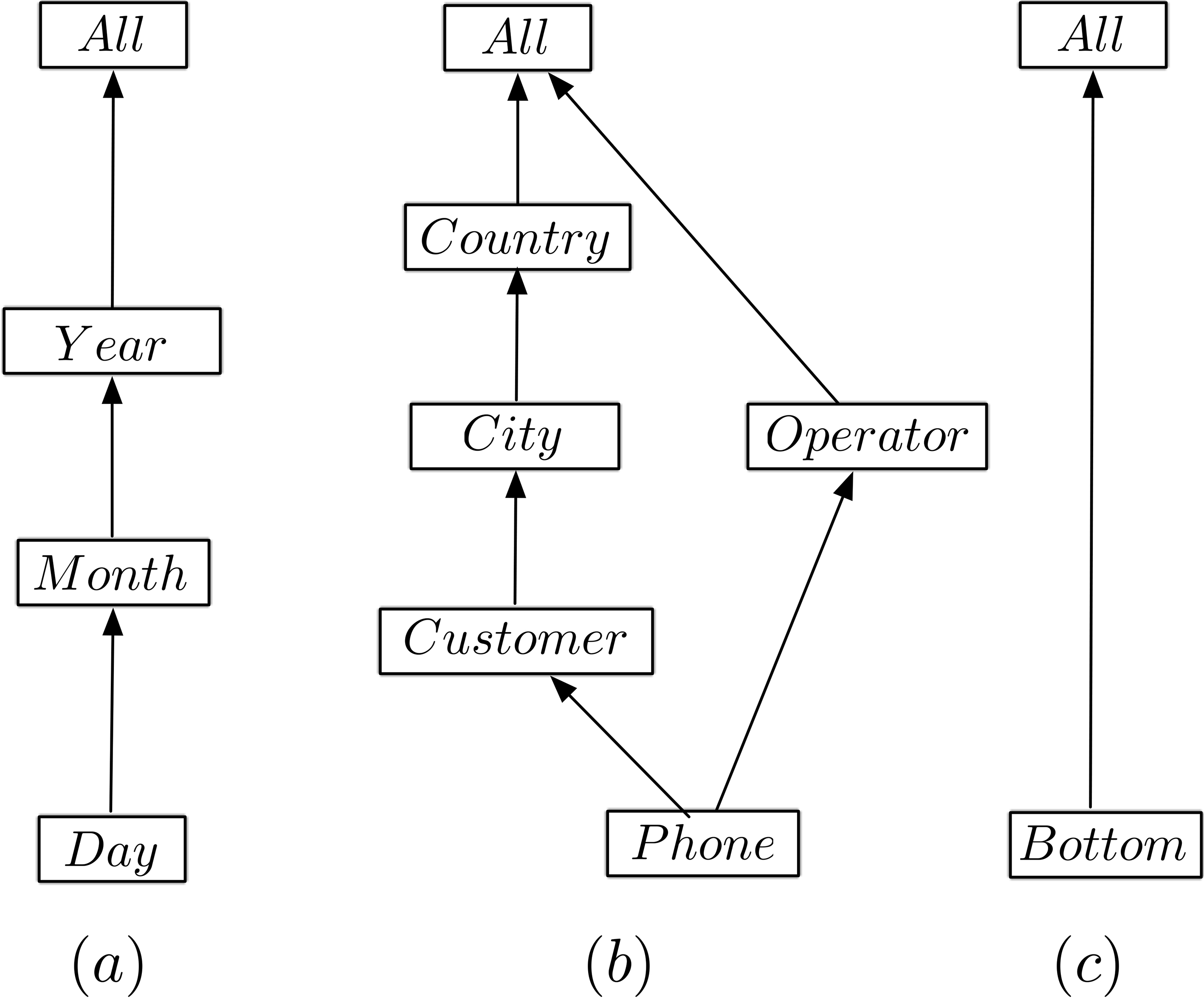
.
Figure 1 depicts the dimension schemas
and
The node Customer is an example of a level in the first of the above hierarchies. For the dimension Time,
(Level, hierarchy, and dimension instances).
Let
A dimension graph (or instance)
where the union is taken over all levels in
If
.
A hierarchy instance
.
Consider dimension Phone whose schema
An example of a dimension instance 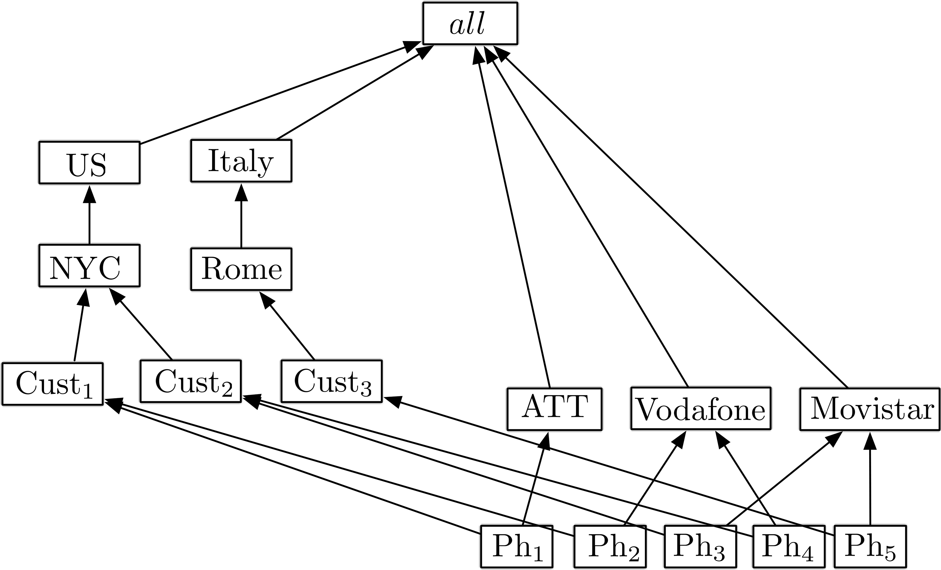
In what follows, “sound” dimension graphs are assumed. In thses graphs, rolling-up from the Bottom level, to the same element along different paths, gives the same result [17], typical in so-called balanced (or homogeneous) dimensions [26].
As a basic data structure for modelling OLAP on graph data, the concept of graphoid is introduced and defined in this section. A graphoid plays the role of a multi-dimensional cuboid in classical OLAP and it is designed to represent the information of the application domain, at a certain level of granularity. Essentially, a graphoid is a node- and edge-labelled directed multi-hypergraph.
In what follows, a collection of dimensions
Attributes
The set of attributes
Node types
Assume a finite, non-empty set
Edge types
Assume the existence of a finite, non-empty set
It is now possible to define the notion of graphoid.
(Graphoid).
Let
Let
The basic graph data that serves as input data to the graph OLAP process, is called the base graph. A base graph plays the role of a multi-dimensional cube in classical OLAP and is designed to contain all the information of the application domain, at the lowest level of granularity.
(Base graph).
Let dimensions
.
The running example used in this paper is aimed at analysing calls between customers of phone lines; lines correspond to different operators. Examples 1 and 2 showed some of the dimensions used as background information. Next, the call information is shown, represented as a graph. The Phone dimension plays the roles of the calling line and the callee lines (this is called a role-playing dimension in the OLAP literature [26]). The information in the hyperedges reflects the total duration of the calls between two or more phone numbers on a given day. Figure 3 shows an example of a base graph, where
Basic phone call data as a base graph.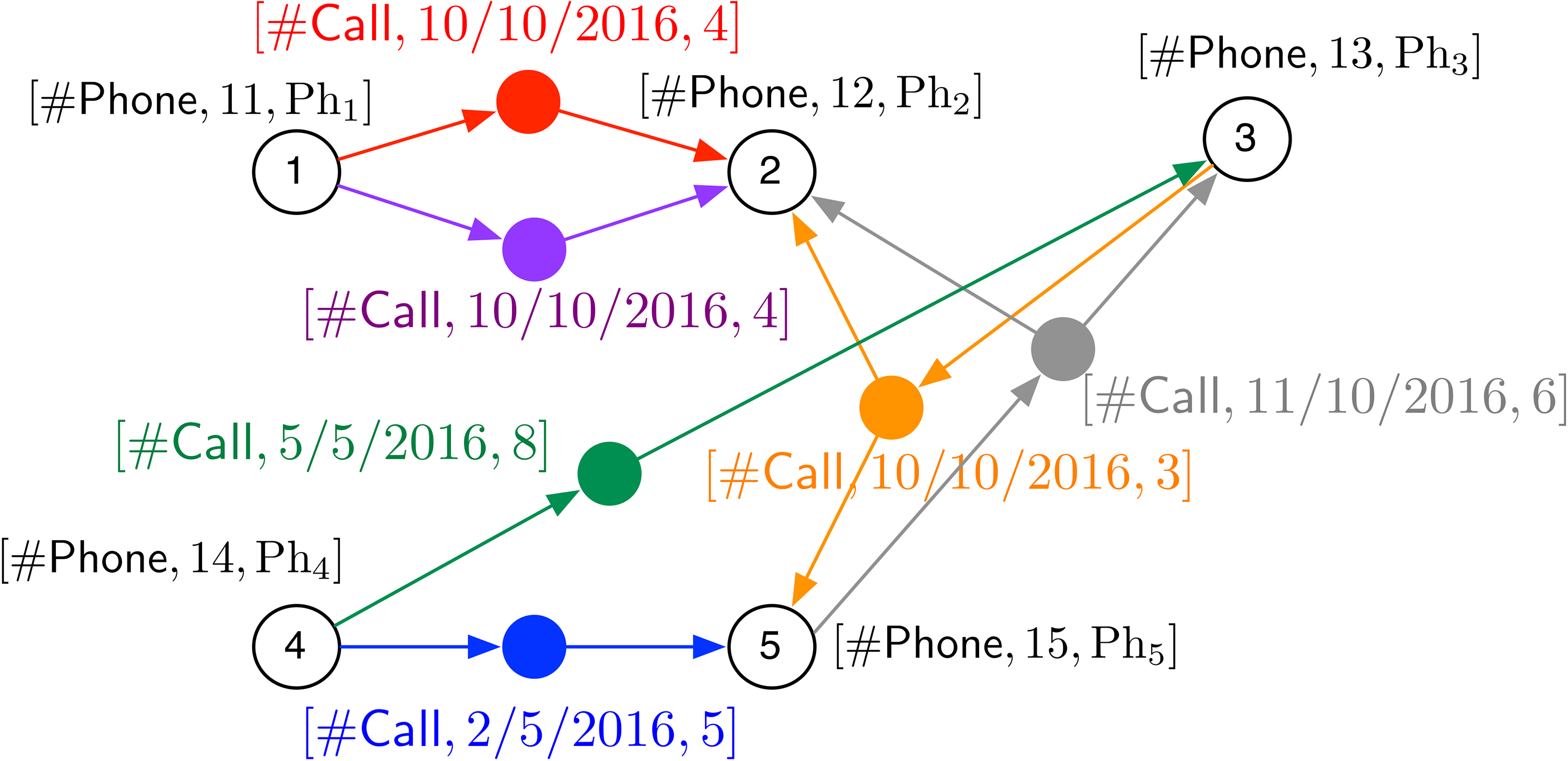
Hyperedges represent phone calls, which most of the time involve two phones, but which may also involve multiple phones, representing so-called “group calls.” So, edges are all of the same type
The nodes of
Note that, although the base graph plays the role of a multi-dimensional cube in classical OLAP (or a fact table in relational OLAP), a key difference is that this cube has a variable number of “axes”, since it can represent facts including a variable number of dimensions. The next example discusses two graphoids whose dimensions are at different levels of granularity. Later it will be explained how these graphoids can be obtained from the base one.
.
Continuing with Example 3, consider two available dimensions, namely
A 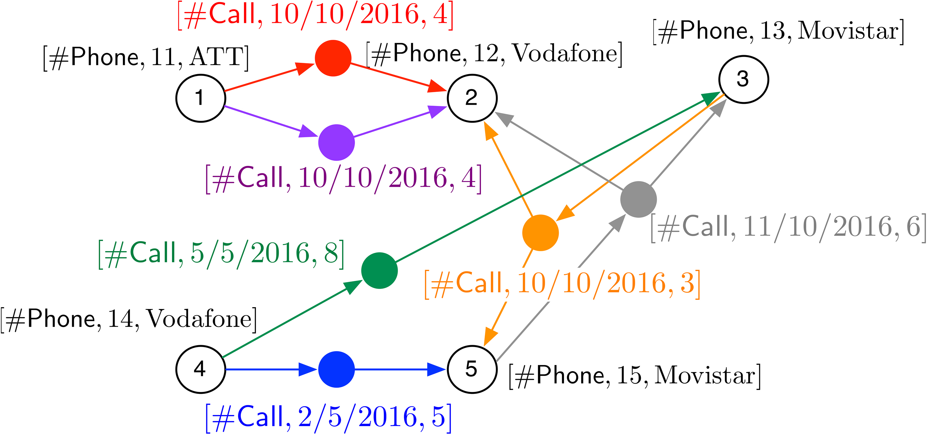
An alternative 
Figure 5 shows an alternative
.
Nodes are assumed to represent basic objects in the modelled application world. These objects are given by a number of descriptive attributes. Measure information, typically present in an OLAP setting to quantify facts, is, in this philosophy, represented as attributes on the hyperedges. The call duration is an example of a measure that is placed on edges of the type Call. However, the above definition also allows for node attributes to be dimensions that contain measure information. Consider a slightly modified situation in which an object of type
(a) A node with label 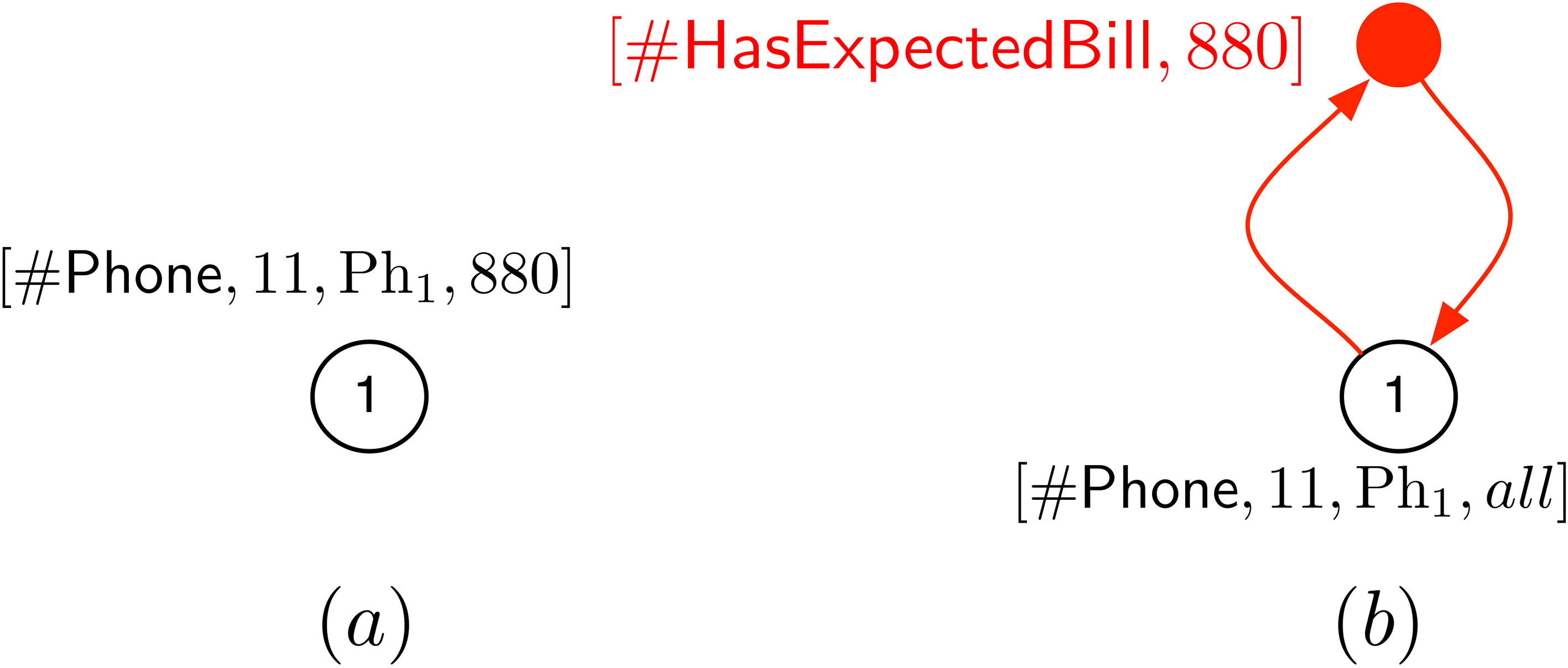
In this section, the notion of minimal
(Minimal graphoid).
Let
.
The set
Proposition 1 immediately follows from Definition 5.
.
For any
.
The two
For any
.
It is easy to see that the minimal
In this section, the operations that compose the graph-OLAP language over graphoids are defined. Section 5 will show that these operations can simulate the typical OLAP operations on cubes.
Climb
The Climb-operation, intuitively, allows to define graphs at different levels of granularity, based on the background dimensions.
(Climb).
Assume a
The node-climb-operation of
The edge-climb-operation of
.
Applying to the graphoid
.
If a dimension
Grouping
The Group-operation, both on nodes and on edges, is defined in this section.
(Grouping).
Assume a
The node-grouping of
The edge-grouping of
.
Applying to the graphoid
Aggregate
In this section, the Aggr-operation on measures stored in edges is defined.
(Aggregate).
Given a minimal
.
Applying the operation
.
To aggregate multiple dimensions
.
Although the operations Climb, Group, and Aggr, are not present in classic relational OLAP, they are included here for several reasons: first, they can be useful when operating on graphs in practice; second, they facilitate and make it simple the definition of the Roll-up operation, that otherwise could be unnecessarily difficult to express. ∎
Roll-Up
The operations defined above allow defining the Roll-Up-operation over dimensions and measures stored in edges, as explained next.
(Roll-Up).
Assume a
is defined as
∎
.
Applying to the graphoid depicted in Fig. 5 the operation
The result of the operation 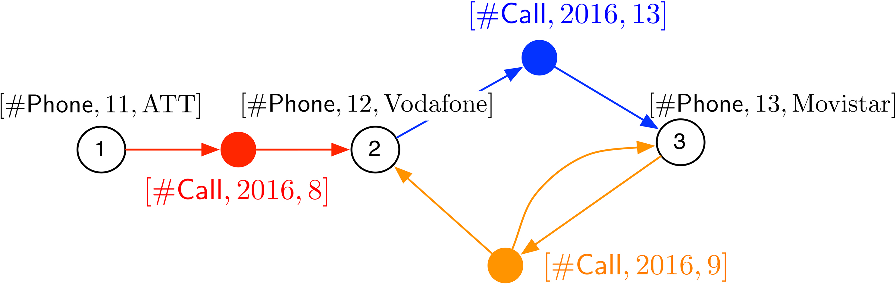
.
To apply the climbing in the roll-up operation to the nodes and edges of all possible types, the shorthand “
The Drill-Down-operation does the opposite of Roll-Up,11
Actually, this is true for a sequence of roll-up and drill-down operations such that there are no slicing or dicing operations (explained in Sections 4.6 and 4.7) in-between. However, for the sake of simplicity, and without loss of generality, in this paper it is assumed that roll-up and drill-down are the inverse of each other.
is defined as
Given the above, in what follows the discussion is limited to the Roll-Up-operation.
The Dice-operation over a graphoid, produces a subgraphoid that satisfies a Boolean condition
where all
Before giving the definition of the Dice-operation, it must be explained what does it mean that a hyperedge
(Dice).
Assume a
.
Applying the operation
(a) The result of the operation 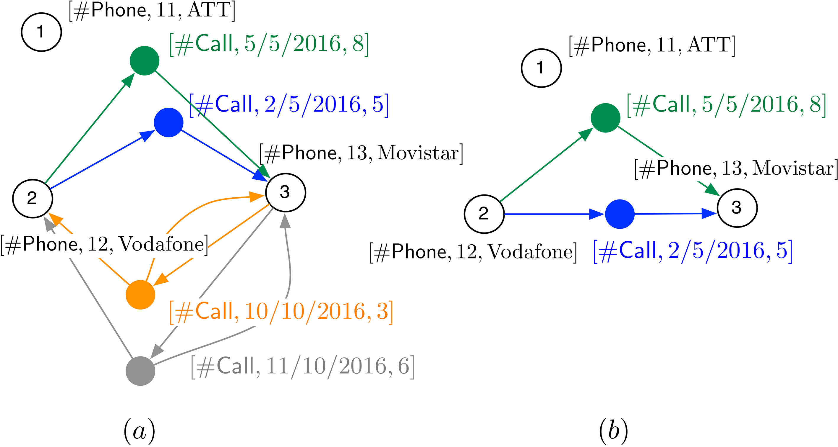
Intuitively, the Slice operation eliminates the references to a dimension in a graphoid. The formal definition follows.
(Slice).
Assume a
.
Applying the operation
The result of the operation 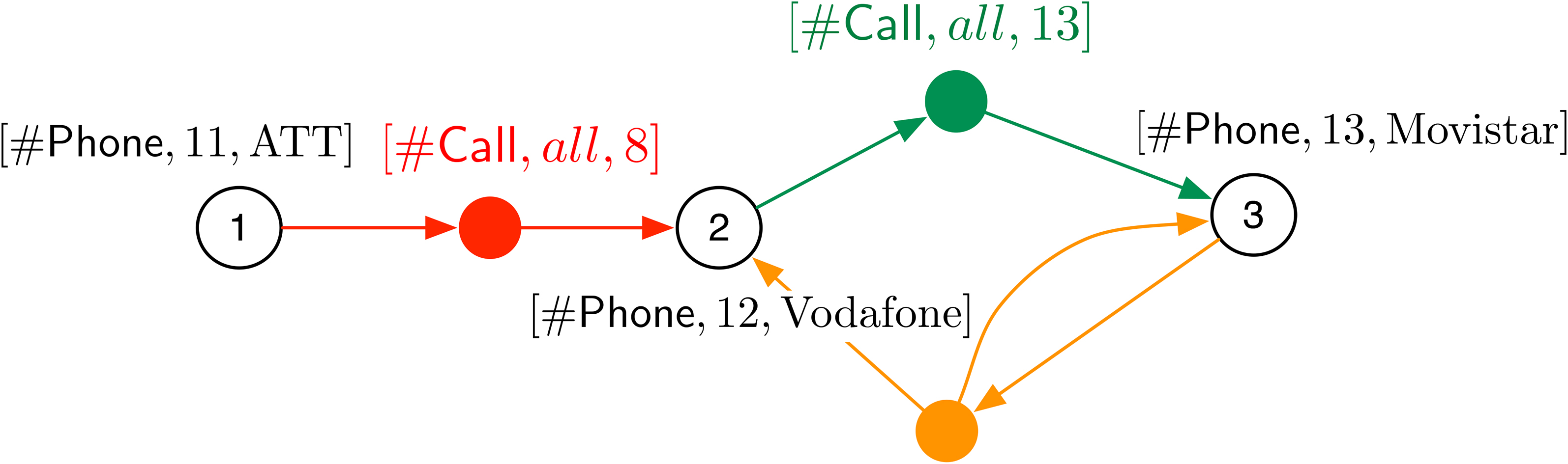
The n-Delete-operation over a graphoid, deletes all nodes of a certain type and delete, in the source and target set of all edges, the nodes of this type. Again, although this operation is not present in classic OLAP, it is needed to simulate the classic OLAP slice operation, as will become clear in Section 5.2.
(Node-delete).
Assume a
.
When a graphoid contains only nodes of one type, as in Fig. 3, the result of the deletion of a node is, obviously, the empty graph. In the graphoid of Fig. 11 (explained later), the result of
Classical OLAP cubes as a special case of OLAP graphs
This section explains how the classical cube-based OLAP model can be represented in the graphoid OLAP model. It is also shown that the classical OLAP-operations Roll-Up, Drill-Down, Slice and Dice can be simulated by the graphoid OLAP-operations defined in Section 4.
A discussion on modelling cubes as graphoids
Figure 10 illustrates a typical example of an OLAP cube with dimensions
An example of a Sales data cube with one measure: 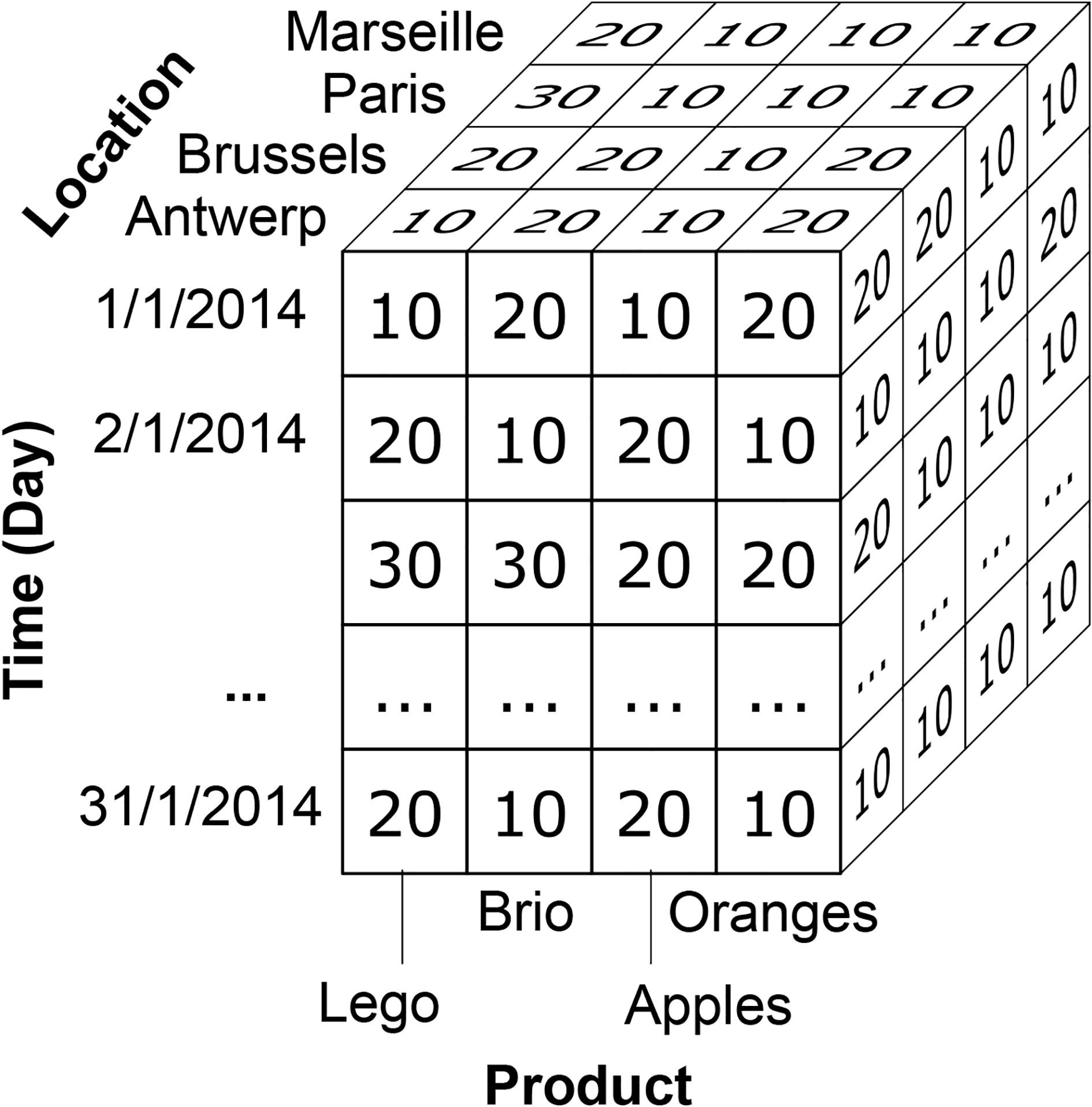
Star-representation of the fact 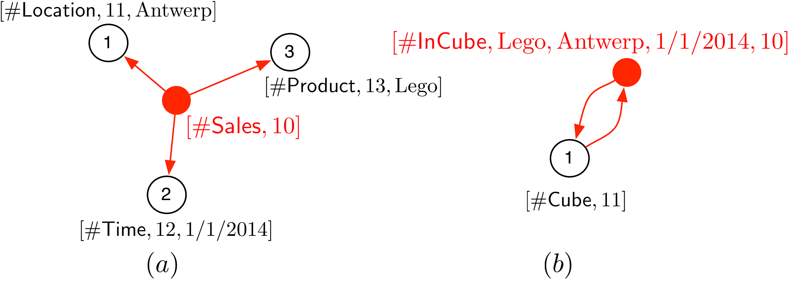
Figure 11a shows nodes 1, 2 and 3, of types
A more compact representation is shown in Fig. 11b. Here, there is only one node, of type
In between the two alternatives above, there are, obviously, more modelling possibilities. The next section will show that the graphoid OLAP-operations presented in Section 4, are at least as powerful as the classical OLAP-operations of the classical cube model. The proof will assume the star-representation of data cubes in the graphoid model (Fig. 11a).
A classical data cube is based on dimensions
(Star-graphoid).
Let
For For each cell
Now, the main theorem of this section is stated.
.
The cube OLAP-operations Roll-Up, Drill-Down, Slice and Dice can be expressed (or simulated) by OLAP-operations on graphoids.
Proof..
Let
Let
To see the correctness of this claim, the substeps in the above graphoid roll-up are analysed. First,
with
Let
If
If
By a similar reasoning, it can be shown that when
This shows that exactly the edges (labelled
The running example followed so far in this paper will also be used as a case study, in order to evaluate the hypergraph model against the traditional relational OLAP alternative. The example case has many interesting characteristics, such as: (a) Normally it involves huge volumes of data facts (i.e., calls); (b) The number of dimensions involved in facts is variable, since calls may differ from one another in the number of participants; (c) It allows performing not only the typical OLAP operations described in Section 4, over the fact measures, but also to aggregate the graph elements using graph measures like shortest paths, centrality, and so on. Therefore, the case study is appropriate for illustrating and discussing the graphoid model usefulness in two situations: (a) The classic OLAP scenario, where the relational model is normally used; and (b) A Graph OLAP scenario, where graph metrics are aggregated. The hypothesis to be tested here is that, although the relational OLAP alternative works better in scenario (a), when facts have a fixed dimensionality (e.g., when all calls in the database involve the same number of participants), the graphoid model is competitive when the number of dimensions is variable, and definitely better for scenario (b), where queries compute aggregations over graph metrics.
The dataset to analyse consists of group calls between phone lines, where a line cannot call itself, and the analyst also needs to identify the line who started the call. The schemas of the background dimensions are the ones in Fig. 1, with small changes that will be explained below. Facts are similar to the ones in Fig. 3.
Although performing an exhaustive experimental study is beyond the scope of this paper, and will be part of future work, this section aims at analysing the plausibility of the graph model to become a better solution that the relational model for the kinds of problems where factual data are naturally represented as graphs. For this, the graphoid model are compared against the relational alternative containing exactly the same data. First, two alternative relational OLAP representations are implemented on a PostgreSQL database, and three synthetic datasets of different sizes are produced and loaded into both representations. Then, the same datasets are loaded into a graph database. Neo4j is used for this purpose, and queries are written in Cypher, Neo4j’s high level query language.12
Since the relational design may impact in query performance, two alternative designs for the fact table are implemented in order to provide a fair comparison. In both cases, the fact table schema is the following:
The meaning of the attributes is:
CallId: Call identifier; CallerId: The identifier of the line which initiated the call; StartTime, EndTime: Initial and final instants of the call; Duration: Attribute precomputed as (StartTime – EndTime).
Although the schemas are the same in both cases, the instances differ from each other. In one case, a call between phone
As expressed above, the background dimensions are the same of Fig. 1. There are two slight differences, however, for practical reasons. First, for the Time dimension, the bottom level has granularity Timestamp, since the StartTime and EndTime attributes in the fact tables have that granularity. That means, a new level is added to the dimension. Second, in the Phone dimension the bottom level is the phone identifier, denoted Id, which rolls up to the line number, denoted Number. This is because the caller and the callee are represented as integers, as usual in real world data warehouses. The Phone dimension is represented in a single table, keeping the constraints indicated by the hierarchies. This representation (i.e., Star) was chosen to provide a fair comparison. In summary, the dimension table schema is
The logical model for the graphoid representing the calls (i.e., the base graphoid), is similar to the one depicted in Fig. 3. There are two main entity nodes, namely
Portion of the call-graph.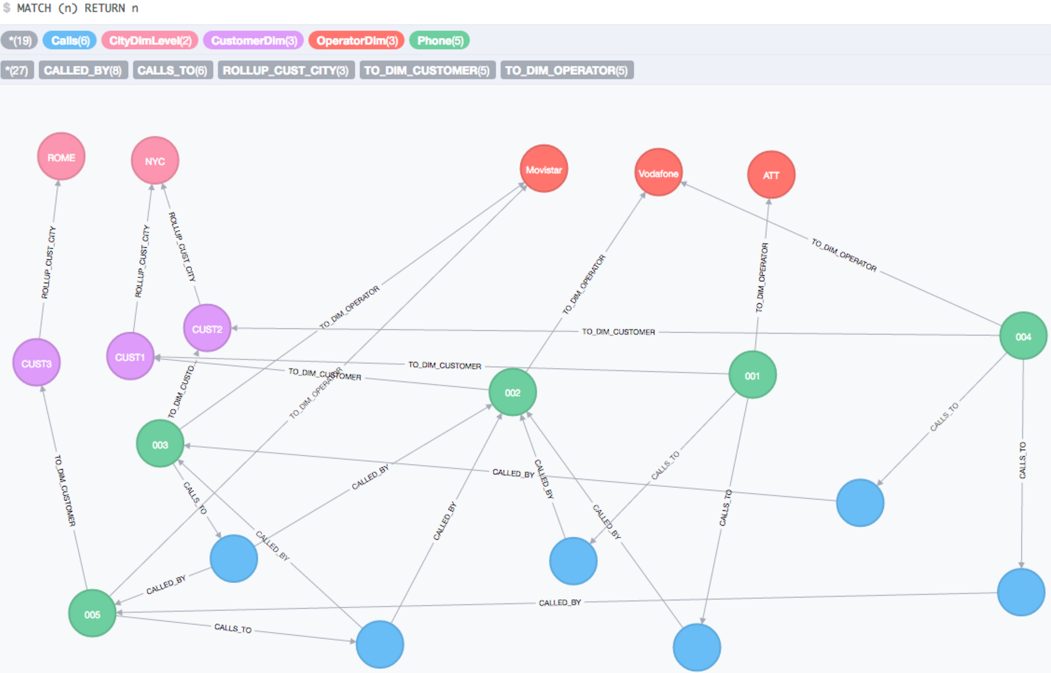
For the relational representation, synthetic datasets of two different sizes are generated and loaded into a PostgreSQL database. Table 1 depicts the sizes of the datasets. The first column shows the number of tuples in the Calls fact table. The second column shows the number of tuples in the Calls-alt fact table. The third column indicates the number of calls (only one column, since the number of calls is the same in both versions), and the fourth column tells the number of tuples in the Phone dimension table.
Dataset sizes for the relational representation
Dataset sizes for the relational representation
For the graph representation, Table 2 depicts the main numbers of elements in the Neo4j graph.
Dataset sizes for the graph representation
Query 1 – Calls representation.
This section shows how different kinds of complex analytical queries can be expressed and executed over the three representations described above. Four kinds of OLAP queries are discussed: (a) Queries where the aggregations are performed for pairs of objects (e.g., phone lines, persons, etc.); (b) Queries where aggregations are performed in groups of N objects, where
.
Average duration of the calls between groups of N phone lines.
This query computes all the
Query 1 – Cypher query for 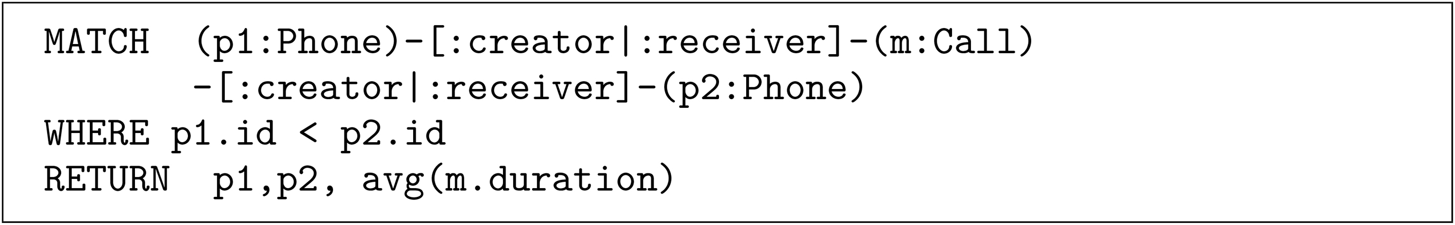
Query 1 – Cypher query for 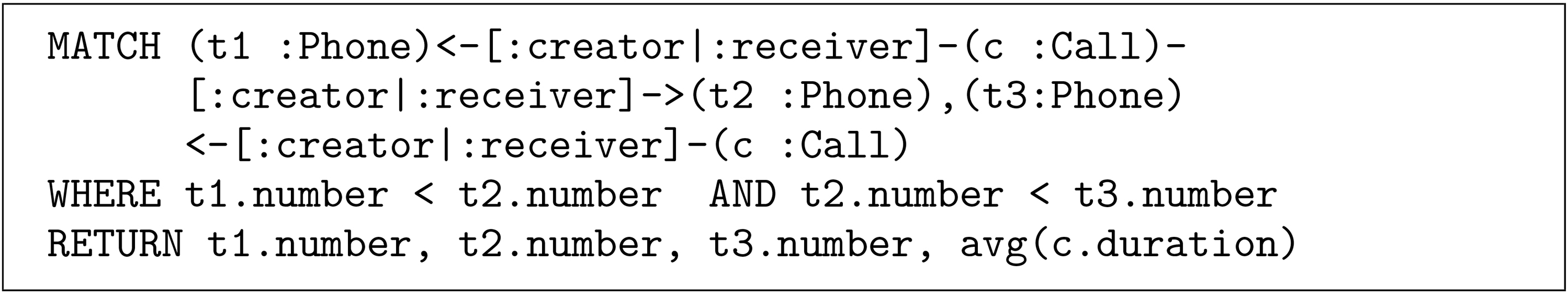
.
Average duration of the calls between groups of N users.
Figure 16 shows the Cypher query for
Query 2 – Cypher for 
.
Average duration of the calls between groups of N operators.
This analyses a roll-up to the level Operator, which has less instance members than the level User addressed in Query 2.
.
For each pair of Phones in the Calls graph, compute the shortest path between them.
This query aims at analysing the connections between phone line users, and has many real-world applications (for example, to investigate calls made between two persons who use a third one as an intermediary). From a technical point of view, this is an aggregation over the whole graph, using as a metric the shortest path between every pair of nodes. Figure 17 shows the corresponding Cypher query.
Finally, the following queries combine the computation of graph metrics together with roll-up and dice operations.
.
Compute the shortest path between pairs
.
Compute the shortest path between pairs
.
Compute the shortest path between pairs
Table 3 shows the results of the experiments. The tests were ran on machine with a i7-6700 processor and 12 GB of RAM, and 250 GB disk (actually, a virtual node in a cluster). The execution times are depicted, and are the averages of five runs of each experiment, expressed in seconds. The winning alternatives are marked in boldface, for clarity.
Experimental results (running times in seconds)
Experimental results (running times in seconds)
Query 3 – Cypher expression.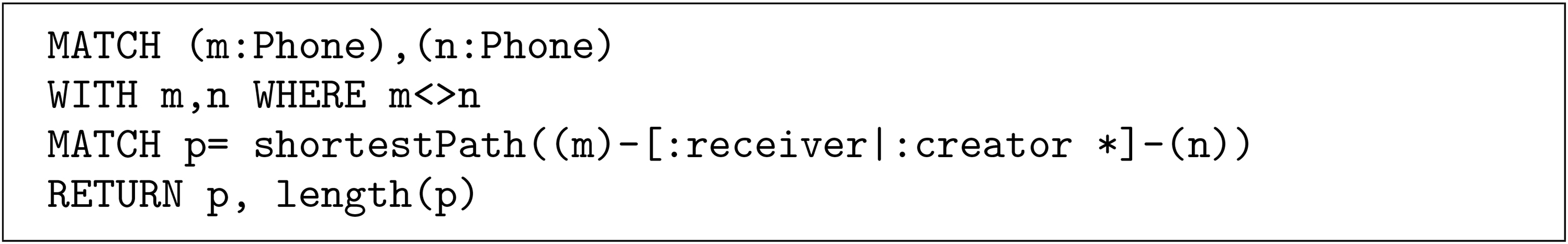
In Table 3 it can be seen that running traditional OLAP queries, like Query 1, Query 2 and Query 3, takes approximately the same time in the relational and graphoid models, with a slight advantage for the former. Further, it can be seen that for Queries 2 and 3, which include a roll-up, results are very similar, and even Neo4j wins here in some cases. In Query 1, which is an aggregation over the fact graph, the relational alternatives work better.13
It is worth noting that Neo4j (and graph databases in general) is a novel database, whose query optimization strategy is still very basic. On the contrary, relational databases are mature technologies, and query optimization is very efficient indeed. Further, for the experiments presented here, the PostgreSQL databases have been tuned to perform in the best possible way. In this sense, Neo4j’s performance for typical OLAP queries is, in some sense, penalized.
This paper presented a data model for graph analysis based on node- and edge-labelled directed multi-hypergraphs, called graphoids. A collection of OLAP operations, analogous to the ones that apply to data cubes, was formally defined over graphoids. It was also formally proved that the classic data cube model is a particular case of the graphoid data model. As far as the authors are aware of, this is the first proposal that formally addresses the problem of defining OLAP operations over hypergraphs. Supported by this proof, it was shown that the graphoid model can be competitive with the relational implementation of OLAP, but clearly much better when graph operations are used to aggregate graphs. This feature allows devising a general OLAP framework that may cope with the flexible needs of modern data analysis, where data may arrive in different forms. It is worth to remark, once more, that the experiments presented do not pretend to be exhaustive, but a good general indication of the plausibility of the approach, and it is clear that the graph data model provides OLAP with a machinery of more powerful tools than the classic cube data model, which is already good news for the OLAP practitioners.
Building on the results in this paper, future work includes looking for further graph metrics that can be applied to the graphoid model, new case studies, and the study of query optimization strategies. Moreover, the approach can also benefit from tools supporting parallel computation with columnar databases as backends. This can further improve the relational OLAP computation, while keeping the properties of the graphoid model for Graph OLAP queries.
Footnotes
Acknowledgments
Alejandro Vaisman was supported by a travel grant from Hasselt University (Korte verblijven-inkomende mobiliteit, BOF16KV09). He was also partially supported by PICT-2014 Project 0787 and PICT-2017 Project 1054. The authors also thank T. Colloca, S. Ocamica, J. Perez Bodean, and N. Castaño, for their collaboration in the data preparation for the experiments.