Distributed frequent subgraph mining on evolving graph using SPARK

Abstract

Within the graph mining context, frequent subgraph identification plays a key role in retrieving required information or patterns from the huge amount of data in a short period. The problem of finding frequent items in traditional mining changed to the innovation of subgraphs that recurrently occurs in graph datasets containing a single huge graph. Majority of the existing methods target static graphs, and the distributed solution for dynamic graphs has not been explored. But, in modern applications like Facebook, robotics utilizes large evolving graphs. The goal is to design a method to find recurrent subgraphs from a single large evolving graph. In this research paper, a novel approach is proposed called DFSME, which uses SPARK to discover frequent subgraphs from an evolving graph in a distributed environment. DFSME maintains a set of subgraphs between frequent and infrequent subgraphs, which is used to decrease the search space. Our experiments with synthetic and real-world datasets authorize the effectiveness of DFSME for mining of recurrent subgraphs from huge evolving graph datasets.

Keywords

Frequent subgraph graph mining big data evolving graph SPARK social network

1. Introduction

Data mining is the method of acquiring information from a vast amount of data. Mining is common in many applications, such as transportation, medicine, social networks, bioinformatics, communication networks, robotics, and link analysis. Multi-relational data mining is a recent research topic, regarding the finding of a pattern from a composite dataset [48]. Extracting knowledge or information from a composite dataset is a difficult task because of its exponent growth. An effective methodology is required to handle such massive data. The graph data structure is the best way to represent complex datasets, and it is incorporated in most applications. In the traditional method, finding frequent items in an evolving database is a hectic task. Similarly, finding recurrent subgraphs from graph dataset is difficult. Frequent subgraph mining (FSM) is the method of identifying entire subgraphs that are recurrent in a graph dataset. To discover recurrent subgraphs, many methodologies have been proposed over the past two decades. Many applications use this frequent subgraph mining technique and achieve maximum utilization. For instance, nuclear smuggling is a hazardous threat in the modern world. Mining the patterns from nuclear smuggling data prevents the threat, and the information garnered can be used for further investigations. Since this data is dynamic, a novel approach is required to handle the data efficiently and effectively. Most professional organizations use configuration management databases to illustrate the IT infrastructure entities and their relationships.

Mining a configuration management database graph for recurrent subgraphs can disclose infrastructure patterns. IT policies can be framed using these patterns. So, FSM is useful and utilized in many fields. To quickly discover subgraphs, a distributed solution is needed. FSM-H and MRFSM were proposed, which uses a MapReduce based framework [7, 35]. But this problem will work for static graphs. Yan and Han investigated recurrent graph-based pattern mining in a graph dataset and used a method called gSpan that discovers frequent items without candidate generation. The Depth-First Search (DFS) lexicographic approach is applied to efficiently mine recurrent subgraphs and map to a unique DFS code. The determined gSpan performs better than FSG and can extract large recurrent subgraphs in a larger graph dataset with fewer minimum supports than prior studies [50]. A sample for frequent subgraph is shown in Fig. 1.

Figure 1.

Example for frequent subgraph.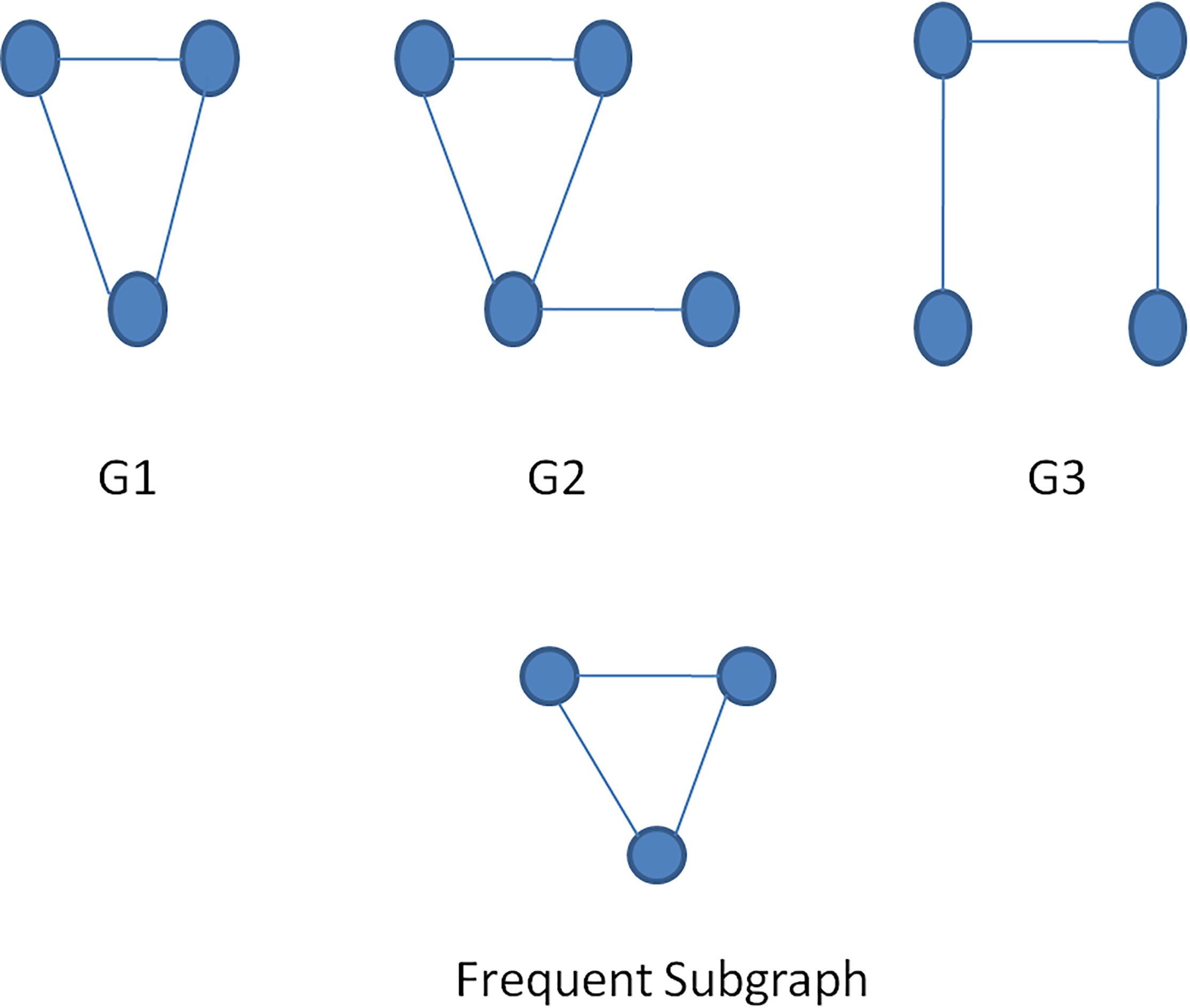

In the above figure, three different graphs represented by G1, G2, and G3 and a recurrent subgraph is shown. This subgraph occurred twice in the given set and also crossed the threshold value to prune the search space. Practically, frequent subgraphs can be easily extended to a very large graph database containing suitably variant labels for edges and vertices [32]. In a distributed environment, input graphs are divided and assigned to diverse worker nodes. Local support count of the subgraph in a portion of the node is not much helpful for determining whether or not the subgraph is recurrent. Aggregation of the count among various nodes is not possible in MapReduce because it doesn’t have any inbuilt system to convey with a global state. Apache Spark with pregel API is more suitable for graph applications.

Contributions to this research article:

•

We proposed a novel approach called Distributed Frequent Subgraph mining on an evolving graph (DFSME) that finds recurrent subgraphs in a distributed manner in less time than the traditional method.

•

We designed an optimized data structure to record and subsequently disseminate the information of the mining process for the recurring iterations.

•

We conducted experiments on big real-world datasets as well as synthetic datasets. DFSME is faster and more accurate than other competitors and scales to much bigger graphs.

This article aims to identify all recurrent subgraphs from a huge evolving graph in a distributed approach. The article is structured as follows: Section 2 discusses existing works in recurrent subgraph mining. Section 3 describes the basic information about the graph and ApacheSpark. Section 4 explains the proposed system, and Section 5 examines the proposed approach’s experiment results. Section 6 deduces the paper with the summary and future work directives.

2. Related works

Extracting the recurrent subgraphs that exist in a graph dataset has been a trend in research on big data. Fast Frequent Subgraph Mining (FFSM) is a technique used to generate candidate graphs (all possible combination with existing entities for example a, b, c, d 4 entities – a, ab, ac, abc…etc.) without duplicates while also avoiding subgraph isomorphism by preserving an embedding set for each recurrent subgraph [26]. But, it is used for small graphs and maintaining a complete set of embeddings leads to memory overhead. Another method, called GREW, is a heuristic algorithm intended to operate on a big graph; it finds patterns related to linked subgraphs that have a huge number of vertex-disjoint embeddings [33]. In some situations, the candidate set is huge, and not all patterns are valuable. So, a new technique has been proposed with approximate algorithms to discover recurrent subgraphs [40]. Dhiman and Jain proposed a filtration method that minimizes the number of candidate subgraphs and dropping the overall time complexity [13]. Nijssen and Kok figured out frequent subgraph mining algorithm called GASTON. It searches frequent paths, frequent trees, and lastly cyclic graphs, which provides results for large molecular databases [37, 38]. The drawback is to navigate the chain of embeddings to get complete information about a particular embedding. The FD-CDS algorithm captures the frequent itemsets and uses the storage composition, called FP-CDS tree, which reflects the frequent itemsets over time. The FP-CDS tree is used to dynamically record the change of the recurrent closed itemsets in a landmark window [36].

Frequent subgraph mining is widely used, but it is difficult to extend to data streams as more information has to be tracked and greater complexity has to be addressed. An effective pattern-tree based structure was developed for mining recurrent patterns from data streams [18]. An efficient bit-sequence representation of items is used to minimize time and memory for sliding windows, making the algorithm significantly faster while consuming less memory than the existing algorithms [34, 47]. Washio and Motoda proposed the AGM algorithm, which uses an adjacency matrix for efficiently mining the association rules amongst the frequently appearing substructure in a given graph dataset [29]. Current techniques address static graphs and not dynamic graphs. So, evolving graphs with edge insertions and deletions need to be considered. Frequent subgraph mining algorithms have been extended to graphs’ time series [8]. Bringmann and Nijssen discussed what is frequent in a single graph. Most of the relational data or hyper-graphs are mapped into multiple-sets, normally called transactional setting. But, some graph databases are found to be difficult to represent, such as web or social media, since it is a single large graph that one may not wish to split it into small parts, which is called a single-graph setting [9]. Kuramochi and Karypis addressed the difficulty of finding every subgraph having many edge-disjoint sets in a big, sparse graph. The proposed algorithm is based on vertical and horizontal paradigms. Results depict that these paradigms show better performance in finding frequent subsets in a real dataset. The vertical paradigm proved to be two to five times faster [31].

The extended Apriori algorithm derives all recurrent induced subgraphs from both directed and undirected graph-structured data [30]. AprioriTid algorithm outperforms AIS and STEM on real-time and synthetic data. The execution time decreased a little with an increase in the number of items in the database. The performance gap increased with an increase in problem size [3]. Graph clustering mostly partitions the objects in a graph database into dissimilar clusters based on vertex-connectivity and neighborhood similarity. To overcome this partition, Seeland et al. proposed a Structural Graph Clustering. This method uses the frequent subgraph miner gSpan, which reduces the time complexity and gives more accurate results by providing overlapping (non-disjoint) and non-exhaustive searches [43]. Finding the threshold of a subgraph from a huge graph is a tough job. The support of a subgraph is the highest independent node set of the overlap graph of the embeddings of the subgraph. This description may become too restrictive; hence, this paper proves that the threshold defined in this way is anti-monotone [17]. Subgraph indexing is a process of finding the entire occurrences of a query graph in a very big connected graph database, but this method is static. Jiong Yang and Wei Jin proposed dynamic indexing of a graph using the BR-indexing algorithm. This is done by constructing a Feature lattice, which maintains and searches the relevant features. Using the overlapping relationship, the index regions are pruned [52]. GraphSig technique converts the given graph into feature vectors where each vector represents an area within the graph. Domain information is used to choose a meaningful feature set. This technique accesses only a little part of the search space and groups all candidate subgraphs into sets based on their similarity. Hence, recurrent subgraph mining can be performed on every set with a high-frequency threshold [41].

Forecasting protein function from protein interaction networks is difficult due to the complex relationship between proteins but can be accomplished by identifying recurrent patterns of useful relations in a protein interaction network [11]. The TSP algorithm mines the patterns which have temporal data and forms a connective subgraph. TSP recursively grows the patterns in the dfs manner. Since TSP works to examine the database once and doesn’t produce needless candidates, the results illustrate that TSP outperforms the modified Apriori on time-efficiency [21]. Graph-based anomaly detection (GBAD) uses a subdue method in all of the three anomaly detections: insertion, deletion, and modification. When implemented in frequent subgraph miners, GBAD algorithms produce a significant increase in performance. GBAD algorithm is applied in emails for identifying insider threats [14]. A closed frequent itemset mining technique can be used instead of a general graph mining algorithm. This assures each discovered graph pattern is connected. The paper concludes that algorithms used on the single relational graph can be re-examined for multiple relational graphs as well [51]. A closed graph mining algorithm is developed by using pruning methods that substantially reduce needless subgraphs and also increases the efficiency of mining. But, to detect one failure condition, half of the performance is sacrificed [49].

The SPIN algorithm mines maximal frequent subgraphs from the graph dataset and decreases the size of the output set and also reduces the mined patterns by many orders of magnitude [25]. An incremental pattern matching algorithm was designed to minimize unnecessary computation. Incremental matching problems are unbounded, but there are some special cases wherein the incremental algorithm gives bounded as well as optimal solutions. The complexity of the solution is independent of the size of the data graph, but this algorithm produces better results than batch algorithms [16]. SSIGRAM, WFSM-MR, and DistGraph are distributed methods which were proposed to find the recurrent subgraphs from a large graph [39, 4, 44, 23, 46, 27, 42, 28]. Moment method is used to find frequent subgraph from a single large graph [10]. Danai Koutra has proposed many techniques for graph processing [22]. The existing methods are consuming too much memory space for pattern mining, and it’s rectified in the proposed system by introducing maximal frequent subgraph set. The time is taken to discover frequent subgraph in the existing system is very high. To overcome the existing limitations, we have proposed a parallel processing method using apache spark. The existing methods are used for a static graph, and parallel computation has been not considered for dynamic graph, so it takes more time. The proposed system identifies frequent patterns from the static graph as well as from dynamic graph and also work is done parallelly to reduce time.

3. Preliminaries

Static graphs are singular, large graphs in which there is no inclusion or exclusion of nodes or edges during the evaluation process.

Definition 1: Static graph

A static graph contains set of nodes, $N$ , set of relations, $R\subseteq N\times N$ , and a function, $F$ , that assign labels to nodes and relations, where $N$ , $R$ , and $F$ are static and $G=(N,R,F)$ .

Recently, most of the applications are dynamic. For example, consider a social network in which many operations are dynamic: new friends are added, some followers are removed, or a profile is modified [1]. So, static is no longer feasible and a dynamic or evolving model suits recent applications and problems.

Definition 2: Evolving graph

An evolving graph or dynamic graph contains set of nodes, $N_{a}$ , set of relations, $R_{a}\subseteq N_{a}\times N_{a}$ , and a function, $L_{a}$ , that assigns labels to nodes and relations, where $N_{a}$ , $R_{a}$ , and $L_{a}$ are dynamic and $G_{a}=(N_{a},R_{a},L_{a})$ . Because of its dynamic property, nodes are added or deleted, edges are added or deleted, and the labeling function, $L_{a}$ , is modified [1].

Definition 3: Candidate graph

Candidate graph is the generation of all possible graph combinations with the existing nodes.

Definition 4: Subgraph

A graph $G^{\prime}=(N^{\prime},R^{\prime})$ is a subgraph of another graph $G=(N,R)$ if and only if

•
$N^{\prime}\subseteq N$ , and
•
$R^{\prime}\subseteq R\wedge((n_{1},n_{2})\in R^{\prime}\to n_{1},n_{2}\in N^{% \prime})$ .

Definition 5: Isomorphism

Two different graphs, A and B, are isomorphic if there is a one-to-one association between the nodes of A and those of B such that the number of relations joining any two nodes of A is equal to the number of relations joining the subsequent nodes of B [6], as revealed in Fig. 2.

Figure 2.
Isomorphic Graphs A and B.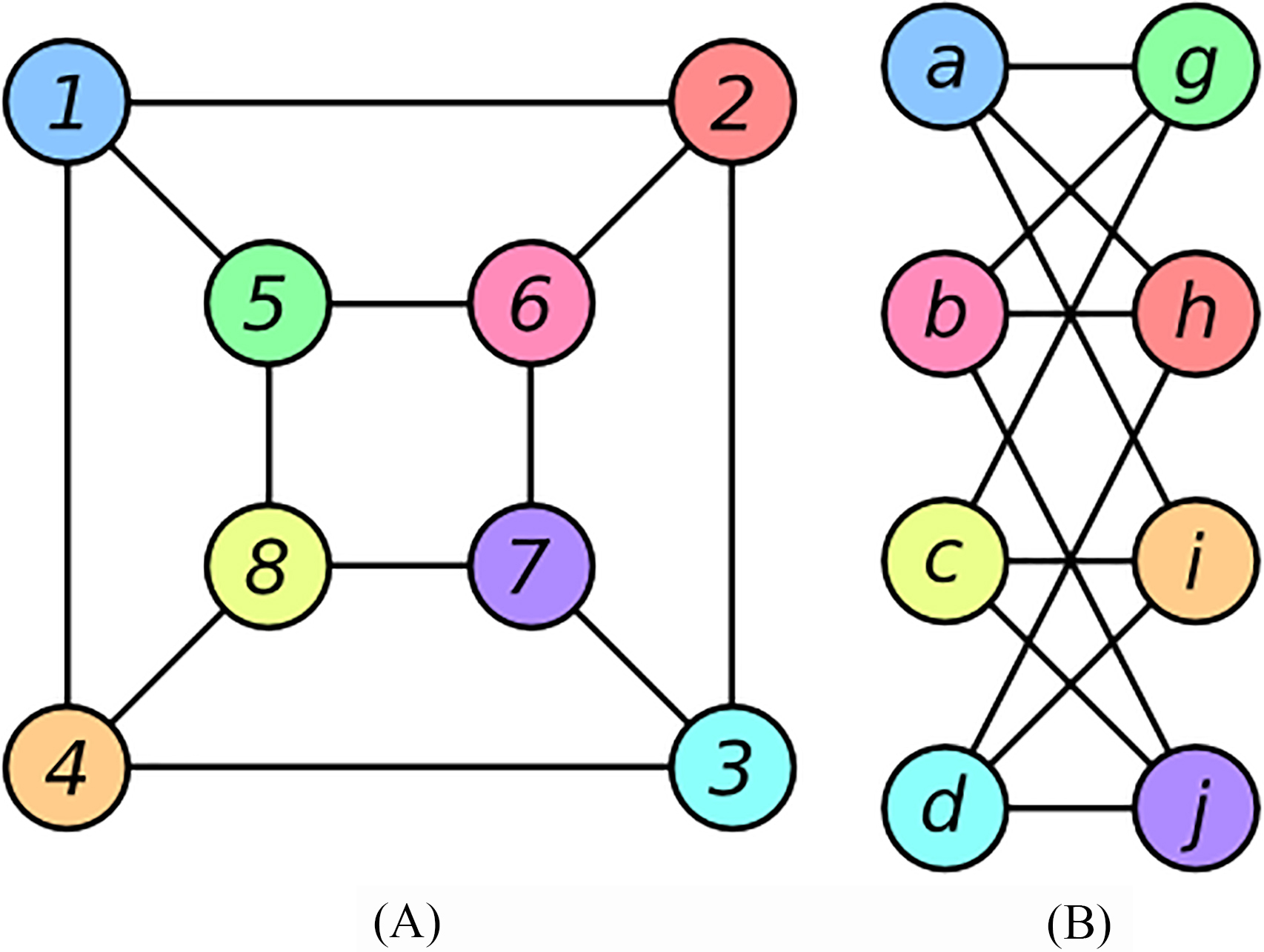

Definition 6: Minimal infrequent and Maximal frequent subgraph

Minimal infrequent subgraph (MIS) is a set of all MIS such that for every $S_{j}$ belonging to MIS, $S_{j}$ is infrequent, and there is no other $S_{k}$ not belonging to frequent subgraphs, where $S_{k}$ is a subgraph of $S_{j}$ . Maximal frequent subgraph (MFS) is a set of all MFS such that $S_{j}$ belongs to MFS, if and only if $S_{j}$ is frequent and there doesn’t exist other $S_{k}$ belonging to frequent subgraphs, where $S_{j}$ is a subgraph of $S_{k}$ . Where ever frequent pattern is applicable use MFS and MIS to minimize search space.

Definition 7: Frequent subgraph or pattern

Frequent subgraph or pattern mining is the problem of identifying all the patterns or subgraphs from the given big dataset, whose support value is equal or more than a certain user-specified level. For a given graph database $DB={\{}B1,\ldots,BK{\}}$ with $K$ graphs and a minimum support threshold $q\in[0,1]$ , $B^{\prime}$ is a frequent subgraph if Support $(B^{\prime}.DB)\geqslant q$ . Pattern mining is useful in many domains, such as sensor networks and medical diagnosis.
3.1 MapReduce and Apache Spark (Pregel API)

MapReduce has to turn out to be an admired platform for analyzing large data. The MapReduce algorithm contains two significant tasks: Map and Reduce.

•
The Mapper accepts a set of data as input and converts it to another form of data, where individual elements are split into tuples.
•
The Reducer takes data from the Mapper and combines those data tuples into a smaller set of tuples.

The reducer job is always performed after the mapper task. Frequent subgraph mining was done using MapReduce, but it doesn’t have any inbuilt system to convey with a global state. So, it takes more time to compute. Apache Spark is a technology designed for rapid computation [45, 20, 2, 5, 12, 19]. It is based on Hadoop MapReduce platform and extends the model to other types of powerful computations. It is well suited for graph applications. So, this model is utilized for the current graph problem. GraphX with Pregel API is used for graph computations. A spark cluster has a Master and numerous Workers. The driver and the executors run their Java processes and users can run them on a horizontal spark cluster or a vertical spark cluster.
4. Distributed frequent subgraph mining

In this research work, a new approach is presented for extracting the subgraphs, which are recurrently occurring in a large evolving single graph or a set of small graphs in a distributed fashion. The DFSME algorithm is proposed to identify the recurrent pattern in a distributed environment called apache spark. Before starting the actual process, it is mandatory to do preparatory tasks. This includes candidate generation, isomorphism checking, and support counting.

4.1 Basic processing in FSM

Usually, recurrent tasks start with a frequent pattern of size one (one edge pattern); later it will be extended until ‘K’. Once a pattern of a different size is identified, for example, size three frequent patterns, the recurrent patterns of size three will merge to provide a new pattern. Check whether the new pattern is frequent or not and avoid duplicate generation because duplication removal will consume the computation time. To avoid it, use rightmost path generation [50] that permits edge is adjoining only with vertices on the rightmost path. The graph isomorphism problem is common in graph processing. Two edges are believed to be of the same class if they are isomorphic to each other in having similar node labels and edge label. This will increase the computation time, to avoid isomorphism use the minimal DFS-code technique [50]. Embedding scheme is used to find frequent subgraphs having support count more than the user specified one. In graph processing, node labels and edge labels are allocated. Then, the embedding list will be created for every candidate graph. For example, three-node or edge subgraph is there, for that embedding is ${\{}u_{11},u_{12},u_{13}{\}}$ , ${\{}u_{11},u_{13},u_{12}{\}}$ , ${\{}u_{12},u_{13},u_{11}{\}}$ . The different combination set contains ${\{}u_{11},u_{12},u_{13}{\}}$ , and remaining combinations are deleted. This allows for the avoidance of duplicate generations. To check the support count, a table will be maintained called MNI anti-monotonic support metrics [9] containing each node count for the particular frequent graph embeddings. A sample frequent subgraph is shown in Fig. 3 for an explanation.

The input graph S in Fig. 4 contains twenty-three nodes and twenty-seven edges unto which labels will be allocated. In this sample, the frequently occurred pattern is { $v_{1},v_{2},v_{3},v_{4}$ , and $v_{5}$ } shown in Fig. 5. One will need to maintain the support count table for every pattern. Once a query is raised, it will check this MNI table and return the pattern that crossed the threshold given by the user. This paper deals with a dynamic graph. So, the count will vary from time t1 to t2. The support count is to be updated based on the embedding scheme. The support count for the subgraph X is 4 for each node. Since it is dynamic, the deletion or the insertion will happen at any time. So, it will check the individual node count and the entire pattern count. Table 1 shows subgraph X embeddings in input graph S when support is equal to 3.

Table 1
MNI table support count

Node	$v_{1}$	$v_{2}$	$v_{3}$	$v_{4}$	$v_{5}$
Label	$u_{1}$	$u_{2}$	$u_{4}$	$u_{3}$	$u_{5}$
Label	$u_{6}$	$u_{9}$	$u_{7}$	$u_{10}$	$u_{8}$
Label	$u_{14}$	$u_{15}$	$u_{16}$	$u_{17}$	$u_{18}$
Label	$u_{19}$	$u_{20}$	$u_{21}$	$u_{22}$	$u_{23}$

Figure 3.

Subgraph X.

Embeddings for $(v_{1})={\{}u_{1},u_{6},u_{14},u_{19}{\}}$ , $(v_{2})={\{}u_{2},u_{9},u_{15},u_{20}{\}}$ , $(v_{3})={\{}u_{4},u_{7},u_{16},u_{21}{\}}$ , $(v_{4})={\{}u_{3},u_{10},u_{17},u_{22}{\}}$ and $(v_{5})={\{}u_{5},u_{8},u_{18},u_{23}{\}}$ . Embeddings and support table is used to find the set of frequent subgraphs for the user given threshold. Maintaining the embedding list is helpful to deal with dynamic graph. For each frequent subgraph, embeddings are maintained in the list format showed above.

Figure 4.

Input raph S.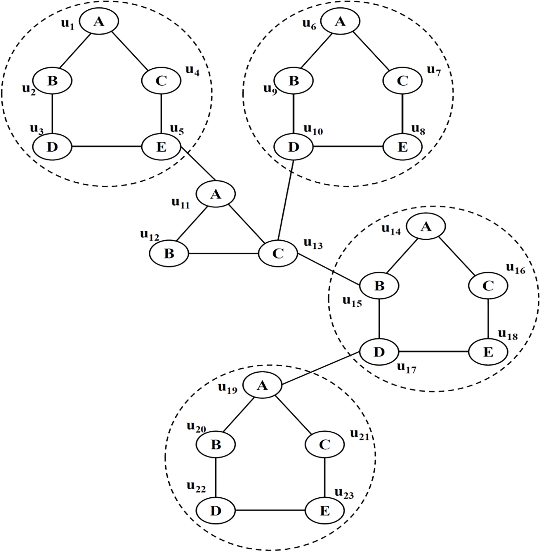

Figure 5.

Architecture of distributed frequent subgraph mining on evolving graph.

4.2 Distributed frequent subgraph mining on evolving graph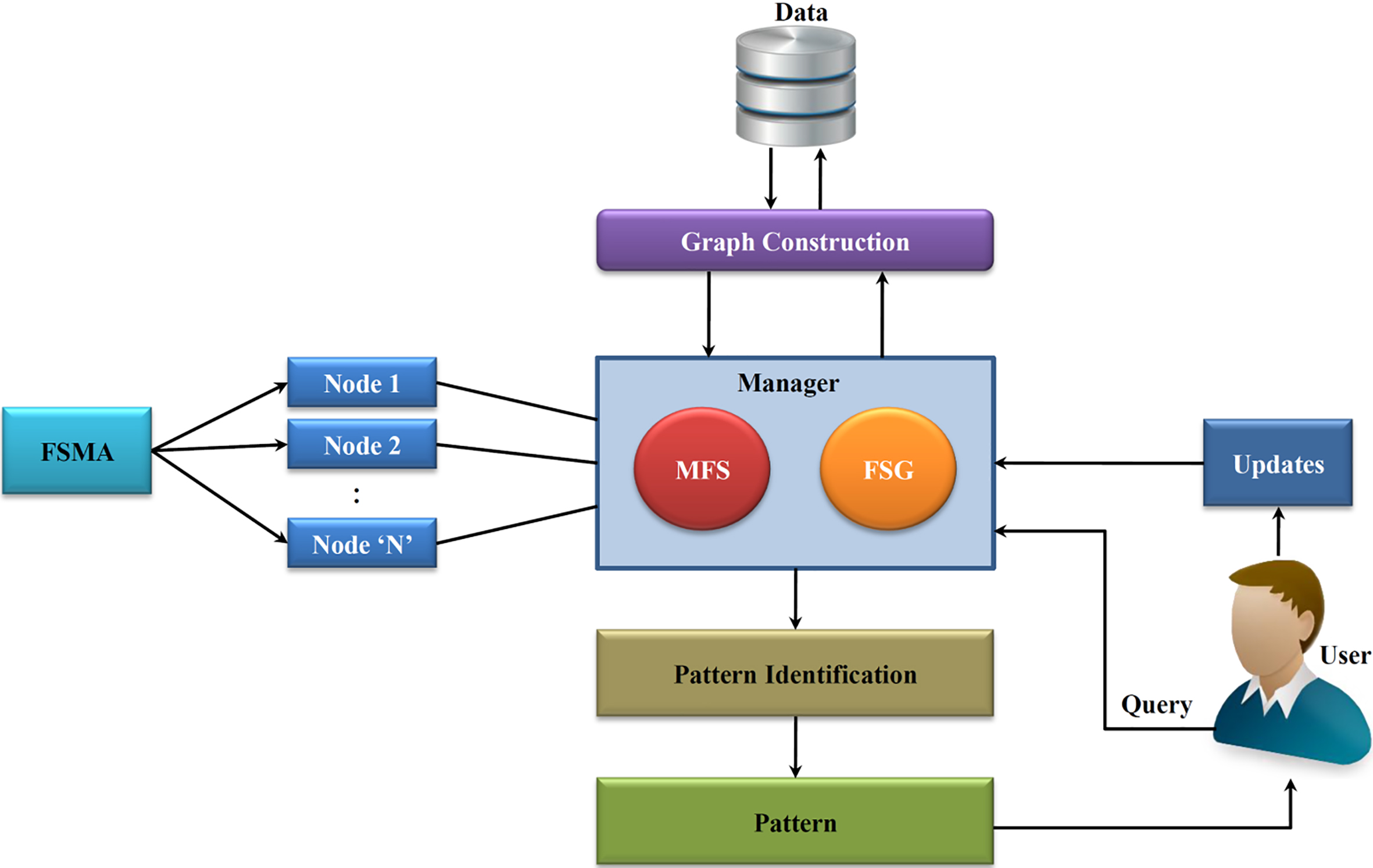

Frequent subgraph mining usually is done for static graphs, but nowadays many applications utilize dynamic data. So, subgraph identification for a dynamic graph is made in a distributed fashion to reduce computation time. The Apache Spark platform is used in this research to accomplish this task. The proposed system was shown in Fig. 5. The components of the proposed method are data collection, graph construction, manager (maintain FSG and MFS), the user (query, updates), distributed FSMA, and pattern recognition. The first step in this process is data collection. Dynamic data can be collected from Twitter, Facebook, Yahoo, and betterenvi datasets. After collecting the dataset, we use the apache spark tool called GraphX to construct the graph with nodes and edges. Nodes will represent a thing or human or machine, and edges will represent its relationships. Since it is dynamic in nature, nodes and edges will be added or deleted at any moment.

The user gives a query to the system (Manager), asking for information or patterns, and the manager will respond to that query. Frequently, data is updated and the graph structure is subsequently modified. The heart of the system is the manager component which identifies the frequent pattern. The manager’s first task is to partition the data in which the total quantity of edges accumulated over the graphs in a partition is close to each other. Apache kMetis library is available and is used for partitioning the given graph [24]. Once the partition task is completed, the graph dataset is allocated to worker nodes. The number of worker nodes required is based on the size of the given data. Each worker node now imposes the FSMA algorithm to find all the possible patterns starting from node one or edge one till ‘K’ node or edge for its own given graph dataset. It will maintain a MNI table for count based on the embedding scheme.

Accordingly, every other worker node maintains a counter table submitted to the manager. Once the manager determines all possible patterns received from all worker nodes, it will eliminate duplicates and consolidate the results. The results are examined with the user threshold value, and finally, the frequent patterns are identified. Since it is dynamic, the graph will change every moment. So, considering the entirety of the data is time-consuming and useless. Re-computation is not required because subgraphs are maintained properly in embeddings format. Therefore, we concentrate only on two sets, frequent subgraphs (FSG) and maximal frequent subgraphs (MFS). A frequent one is above or equal to the threshold set by the user, and the maximal frequent is on the border.

For example, support count is 80 and above, as set by the user. Some subgraphs are present whose count is 78 or 79; in such case, any changes (updates in the graph) will affect only MFS sets, yet any deletions can change the frequent set (FSG). To reduce the search space, this logic of considering only FSG or MFS is imposed. Figure 6 illustrates an example of a dynamic graph at a particular time, t1, where subgraph y is frequent, and z is maximal frequent for a graph G where the support count is 2. At time t2, graph G is updated and now z becomes frequent. Hence, in order to prune search space, considering only MFS without addressing infrequent subgraphs is logical. If new updates arrive, then forward them to the manager; the manager submits the updates to all worker nodes. Then each worker node updates the table with the new data if applicable.

Otherwise, the worker will send back the previous support table. Now, the manager collects the support count from all the workers and check for changes, if any, in the set MFS and FSG. Some subgraphs from the MFS set moves to FSG after the update, and some will move from FSG to MFS. Repeatedly, the process will continue for an evolving graph. Computation time is reduced because of the Apache Spark environment, GraphX, Pregel API and pruning the search space. This approach outperformed other existing approaches, as discussed in the next section. The manager component does two tasks. First, it distributes the task to worker nodes and then receives the count. Next, the manager consolidates the count and checks and maintains frequent and maximal frequent lists. The manager will respond to the user query, giving the pattern or information required for the user to make a further decision. The pseudo code represented below Algorithm 1 will give a detailed description of the proposed approach.

Figure 6.

(a) Dynamic graph at different time. (b) Subgraph Y. (c) Subgraph Z.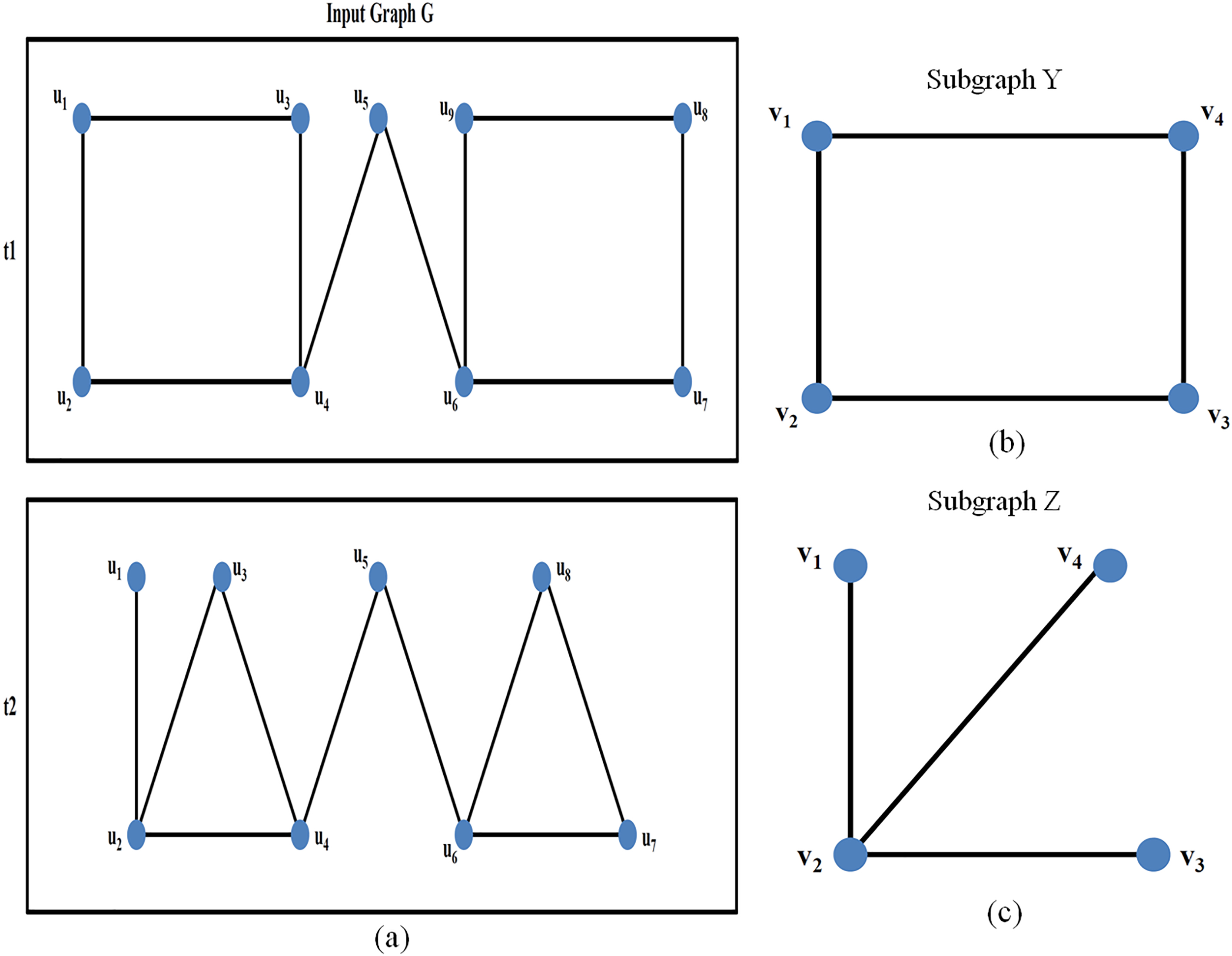

Algorithm 1: Frequent Subgraph Mining on Evolving Graph
1. MFS $\leftarrow\Phi$
2. Graphs $\leftarrow\Phi$
3. For all edges edge in input Graph G do:
4. New_graph $\leftarrow$ createGraph (edge)
5. Add New_graph to Graphs
6. While Graphs has more elements:
7. G $=$ getNextElement (Graphs)
8. If isFrequent (G, r) then:
9. extendedGraph $=$ extend (G)
10. Add extendedGraph to Graphs
11. Add G to MFS
12. For U in updates:
13. If U is vertex addition:
14. changedVertex $=$ U.vertex
15. changedLabel $=$ changedVertex.Label
16. For G in Graphs:
17. If G is the graph with max edges and contains changedLabel:
18. addVertex (changedVertex, G)
19. If isFrequent (G, r) then:
20. extendedGraph $=$ extend (G)
21. Add extendedGraph to Graphs
22. Add G to MFS
23. If U is edge addition:
24. changedFromLabel $=$ U.edge.from.Label
25. changedToLabel $=$ U.edge.to.Label
26. changedEdge $=$ U.edge
27. For g in Graphs:
28. If G is the graph with max edges and contains changedFromLabel and ChangedToLabel:
29. addEdge (changedEdge, G)
30. If isFrequent (G, r) then:
31. extendedGraph $=$ extend (G)
32. Add extendedGraph to Graphs
33. Add G to MFS
34. If U is vertex deletion:
35. deletedVertex $=$ U.vertex
36. For G in MFS:
37. If G.contains (deletedVertex):
38. G.removeVertex (deletedVertex)
39. If isFrequent (G, r) then:
40. extendedGraph $=$ extend (G)
41. Add extendedGraph to Graphs
42. Add G to MFS
43. Else:
44. removeGraph (MFS, G)
45. If U is edge deletion:
46. deletedEdge $=$ U.edge
47. deletedFromVertex $=$ U.edge.from
48. deletedToVertex $=$ U.edge.To
49. For G in MFS:
50. If G contains both deletedFromVertex and deletedToVertex:
51. G.removeEdge (deletedEdge)
52. If isFrequent (G, r) then:
53. extendedGraph $=$ extend (G)
54. Add extendedGraph to Graphs
55. Add G to MFS
56. Else:
57. removeGraph (MFS, G)
58. Return MFS

The algorithm uses the MNI Table to determine whether the subgraph is frequent or not. Every individual edge is taken, and a subgraph is formed that has only one edge and two vertices (lines 3–5). Then the occurrences of the similar graph (graph isomorphism with two different vertex labels and an edge connecting them) within the input graph is searched and the number of satisfying vertices is obtained. If the quantity of satisfying vertices is larger than the given threshold, then the subgraph is considered to be frequent (line8-isFrequentGraph). createGraph (edge) returns a graph with two vertices connected and the edge involved. All such one edge graphs are stored in an array, and every graph is check for the number of satisfying vertices that decides whether the involved subgraph is frequent or not (line 8). If the graph is frequent, the graph is extended by one more vertex and then added back to the graph (line 9). All frequent subgraphs are immediately stored into an array named MFS (line 11). This algorithm can handle updations on the input graph as it is keeping track of all the possible MFS.

4.2.1 Four cases of updation namely

•
Edge addition

The graph with a maximum number of edges and that contains labels from and to vertices of the added edge is obtained, and the edge added to the graph also obtained (lines 24–29). If the graph is to be frequent, it added to the MFS set and the extended graph is added to the list of graphs (lines 30–33).
•
Vertex addition

The graph with a maximum number of edges and that contains a label of the added vertex is obtained, and that vertex is added to that graph (line 18). If the graph is found to be frequent (line 19), it added to the MFS set and the extended graph is added to the list of graphs (lines 20–22).
•
Edge deletion

The graph with a maximum number of edges and that contains labels from and to vertices of the deleted edge are obtained, and the edge is added to the graph obtained (lines 46–51). If the graph is found to be frequent, it added to the MFS set and the extended graph is added to the list of graphs (lines 52–55). If the graph is not frequent, then the graph is deleted from the MFS list (line 57).
•
Vertex deletion

The graph with a maximum number of edges and that contains a label of the deleted vertex is obtained, and the vertex is deleted from that graph (line 35–38). If the graph is found to be frequent (line 19), it added to the MFS set and the extended graph is added to the list of graphs (lines 39–42). If the graph is not frequent, then the graph is deleted from the MFS list (line 44).

Algorithm 2: Distributed FSM

Clustermanager (KVPair (x.hash, x.objs)):
1.
Ck $+$ 1 $=$ GetNextCandidate (KVPair) 2.
For all c e Ck $+$ 1
3.
If isIsomorph (c) $=$ true:
4.
If adjacencyList (c).length $>$ 0:
5.
output (c.hash, c.obj)
6.
End if
7.
End if
8.
End loop

Worker (c.hash, $<$ c.objs $>$ ):
1.
For all obj e c.objs:
2.
Supp $+=$ length (obj.OL)
3.
End loop
4.
If supp $>=$ minsup
5.
For all obj e $<$ c.objs $>$
6.
Write (c.hash, obj) to Clustermanager

Cluster-master

Given:

Key: minimum-dfs code

Value: byte stream of pattern object for iteration i-1
1.
pattern $=$ GetNewPattern (value)
2.
GetNewDataStructures (value)
3.
Candidate $=$ GetNewCandidate (pattern)
4.
For all Pi in P:
5.
If ifIsomorphism (Pi):
6.
If length (Pi, OL) $>$ 0:
7.
i_key $=$ generateCode (Pi)
8.
i_value $=$ GetSerialized (Pi)
9.
emit (i_key,i_value)

Cluster-worker

Given:

Key: minimum-dfs code

Values: List of byte stream of a pattern object in all partitions
1.
For value in values:
2.
Support $+=$ getSupport (value)
3.
If supp $>=$ threshold
4.
For value in values:
5.
write (key, value)

The explanation for the above-represented Algorithm 2 is discussed here; the task is done in a distributed environment using SPARK. The manager component contains DFSME that assigns the task to the Cluster-manager. The Cluster-manager distributes the task to every worker. In the Cluster-manager, a key-value pair is a dictionary of elements with the hash value of the graph as its key and object as the value. Every candidate of length k-1 is iterated and checked for isomorphism. If their corresponding adjacency list has elements, then the hash and the object are passed to the worker. The worker calculates the count of each generated subgraphs and the key-value pair containing the hash and object is passed to the Cluster Manager. Hash is calculated for every candidate subgraph so that while comparing them, it is not necessary to go through every element in the subgraph.

The worker returns all possible subgraphs to the cluster-manager, which in turn forwards the information to the manager. DFSME, which is running in the manager, uses the support table MNI to determine whether the subgraph is frequent or not. The occurrences of similar subgraph within the input graph are searched, and the number of satisfying vertices is obtained. If the quantity of satisfying vertices is larger than the given threshold, then the subgraph is considered to be frequent. All frequent subgraphs are immediately stored into an array named FSG and some subgraphs near to threshold stored in graphs, i.e. MFS. This algorithm can handle updates in the input graph as it is keeping track of all possible FSG. If any addition occurs as an update, the MFS sets that are affected by the update, if it has the particular edge and vertices, are accordingly updated and checked again using the isFrequent (graph, r) and added to FSG if it is frequent.

The deletion updates can cause some changes to the existing FSG graphs that can make the individual subgraph no longer frequent or potentially moved to MFS. Hence, after performing the updates, the graph needs to be checked using isFrequent (graph, r) method and removed if found infrequent. This process will continue indefinitely because it is evolving every moment. Finally, frequent patterns identified based on the requirement of the user will be delivered. Most of the existing algorithms are not scalable, it works only for sparse graph, and it won’t find the complete set of subgraphs and takes too much time for computation. Only minimal patterns are identified by the existing methods, but DFSME identifies all important patterns for the user given threshold, and the proposed work is more scalable. DFSME identifies patterns if the given input graph is larger and dynamic.
5. Experimental evaluation

Algorithm 2: Distributed FSM
Clustermanager (KVPair (x.hash, x.objs)): 1. Ck $+$ 1 $=$ GetNextCandidate (KVPair) 2. For all c e Ck $+$ 1 3. If isIsomorph (c) $=$ true: 4. If adjacencyList (c).length $>$ 0: 5. output (c.hash, c.obj) 6. End if 7. End if 8. End loop
Worker (c.hash, $<$ c.objs $>$ ): 1. For all obj e c.objs: 2. Supp $+=$ length (obj.OL) 3. End loop 4. If supp $>=$ minsup 5. For all obj e $<$ c.objs $>$ 6. Write (c.hash, obj) to Clustermanager
Cluster-master
Given:
Key: minimum-dfs code
Value: byte stream of pattern object for iteration i-1 1. pattern $=$ GetNewPattern (value) 2. GetNewDataStructures (value) 3. Candidate $=$ GetNewCandidate (pattern) 4. For all Pi in P: 5. If ifIsomorphism (Pi): 6. If length (Pi, OL) $>$ 0: 7. i_key $=$ generateCode (Pi) 8. i_value $=$ GetSerialized (Pi) 9. emit (i_key,i_value)
Cluster-worker
Given:
Key: minimum-dfs code
Values: List of byte stream of a pattern object in all partitions 1. For value in values: 2. Support $+=$ getSupport (value) 3. If supp $>=$ threshold 4. For value in values: 5. write (key, value)

This section compares the performance of the proposed work with existing methodologies. The performance is evaluated using real graphs collected from Stanford University datasets (https://snap.stanford. edu/data/). These datasets are used to evaluate the effectiveness of the proposed method for identifying frequent patterns. The experiments were conducted on 3 GB RAM and 2.13 GHz Pentium (R) CPU. Apache Spark is used to accomplish the task in a distributed environment. Ten systems (cluster) were used for analysis; the user can create virtual machines for computation. If the volume of data has been increased, parallelly number of machines also increased automatically for computation. Algorithm implementation was done in Python 3.6.5 and the operating system used was Windows 7. Real-world data was used for the experimental purpose, and its characteristics are shown in Table 2. Orkut, twitter, web-google, Friendster, citation data, and road network of California datasets are taken from the Stanford database for the experimental purpose. The experiment compares the efficiency of traditional FSM [15], FSM-H [7], MRFSM [35], with the proposed method DFSME. The Twitter dataset is used here for testing and runtimes of these methods for the user given threshold are computed to prove which is best.

Table 2
Datasets used

Dataset	Graph density	Nodes	Edges	Distinct node labels
Com-Orkut	Dense	3072441	117185083	613
Web-Google	Dense	3774768	16518948	676
Cit-patents	Dense	875713	5105039	408
Roadnet-CA	Dense	1965206	2766607	576
Ego-Twitter	Medium	81306	1768149	325
Com-Friendster	Dense	65608366	1806067135	8385

Figure 7.

Frequent subgraphs of twitter dataset for support count 20%.

5.1 Results and discussion

DFSME was experimented with by changing the support value. When support was set to 10%; 321 frequent one edge subgraphs, 233 frequent two edge subgraphs, and 127 frequent three edge subgraphs were found. When the threshold value is very low, more frequent subgraphs are obtained. The support value was then changed to 20%; 157 frequent one edge subgraphs, 88 frequent two edge subgraphs, and 39 frequent three edge subgraphs were found. For the 60% threshold value, only 15 frequent subgraphs were found. From this observation, it is concluded that an increased minimum support value resulted in a decrease in the number of recurrent subgraphs. Twitter data compose medium density graphs, whereas other datasets are densely populated. Even in other datasets, if the threshold value is low, more frequent subgraphs are obtained and increasing the threshold value results in very few frequent subgraphs. Figure 8 shows some of the frequent subgraphs identified by DFSME for the user given 20% support count of the twitter graph dataset. Figure 7a–d frequent subgraphs indicate that likes for a tweet about a domain.

GraphGen is a tool used to generate synthetic graph datasets. Using GraphGen, some 50000 graphs were generated and 5000 graphs were used for experimentation. Each utilized graph has some 50 nodes and 120 edges. DFSME was applied on this synthetic graph; here too, when the support count was minimum, more frequent subgraphs were obtained. Once the support count was increased, much less frequent subgraphs were obtained. Then, existing methods like FSM, FSM-H, and MRFSM were applied to the Twitter dataset. These methods identifying recurrent subgraphs of different support values but took more time for computation compared to the proposed DFSME algorithm. Figure 8 shows the relationship between minimum support count and time taken by different methods to identify frequent subgraphs for the Twitter dataset. Computation in the proposed methodology was done in a distributed manner using apache spark with pregel API. The task is assigned to worker nodes by cluster-manager, which will send the data back to the manager. The manager consolidates and maintains frequent patterns. The ultimate use of finding frequent patterns is to make decisions or to set policies that depend on the applications.

The distributed frequent subgraph mining on an evolving graph (DFSME) proposed algorithm execution time for twitter dataset is 55.03 minutes. Threshold varied from 10% to 70% for the same dataset; it is observed that time taken gradually decreased. Similarly, the execution time of MRFSM for twitter dataset is 65.06 minutes, for A-FSM its 59.22 minutes and for FSM-H 61.23 minutes. Time taken was gradually decreased according to the varying support count value. For traditional FSM, execution time is 90.56 minutes, as shown in Table 3.

Table 3
Time taken by various algorithms for different support value to identify frequent subgraph on Twitter data

Algorithm	Support value
	10%	20%	30%	40%	50%	60%	70%
	Processing time in minutes
DFSME	55.03	51.11	46.22	40.01	35.89	30.78	24.65
A-FSM	59.22	54.09	49.89	41.64	37.51	33.34	27.58
FSM-H	61.23	57.08	51.96	44.77	40.21	36.9	30.12
MRFSM	65.06	61.22	56.32	50.21	45.03	40.33	34.21
Traditional-FSM	90.56	81.22	70.25	66.025	58.99	48.97	41.22

Figure 8.

Line plot shows the association between the minimum support count and the runtime of DFSME, FSM-H, MRFSM, and Traditional-FSM for the Twitter dataset.

Table 4 shows the runtime taken by each algorithm and DFSME outperforms other existing methods. Twitter is a medium density graph with 81306 nodes, 1768149 edges, and 325 distinct node labels. Consider the comparatively dense graph dataset, web-google, with 3774768 nodes, 16518948 edges, with 676 distinct node labels for the experiment. In this case, DFSME still takes less computation time when compared to Approximate-FSM, FSM-H, MRFSM, and FSM when identifying frequent patterns. DFSME runtime is 77.11 minutes, A-FSM takes 81.03 minutes, FSM-H takes 84.09 minutes, MRFSM takes 91.36 minutes, and traditional FSM takes 115.89 minutes.

Table 4

Comparison of DFSME, FSM-H, A-FSM, MRFSM, and FSM

Dataset	Density	Nodes	Edges	Distinct node labels	Run-time (minutes)
					DFSME	A-FSM	FSM-H	MRFSM	FSM
Ego-Twitter	Medium	81306	1768149	325	55.03	59.22	61.23	65.06	90.56
Web-Google	Dense	3774768	16518948	676	77.11	81.03	84.09	91.36	115.89

Figure 9.

Comparison of DFSME and fullrecompute for updates in Twitter and Web-Google.

The computation completed for the particular twitter dataset will change, as nodes or edges are added to the graph, or some nodes or edges are deleted from the graph because it is evolving. Any new member can be added to twitter at any time, and any relationship (edge) can be deleted at any moment. DFSME handles this dynamic situation efficiently by focusing on only frequent subgraph (FSG) and maximal frequent subgraph (MFS). FSG is above or equal to the threshold set by the user, and maximal frequent is on the border. For example, the support count is 80 and above set by the user. Some subgraphs whose count is 78 or 79 exist; in such case, any new updates in the graph will affect only the MFS set, but any deletions can change the frequent set (FSG). To reduce the search space, logic of considering only FSG or MFS is imposed. Other methods, like traditional FSM, will recompute everything from scratch with every change. Therefore, it will take more time to identify recurrent patterns. Consider the same evolving twitter dataset for comparison between FSM and the proposed DFSME algorithm. When the update is 250 addition of nodes or edges, the fullrecompute method takes 80 ms, but DFSME takes only 9.5 ms. When the update is 500, fullrecompute takes 170 ms, but DFSME takes only 18.9 ms. When the update is 750, fullrecompute takes 255 ms, but DFSME takes only 28.1 ms.

For twitter dataset in deletion, when the update is 250, fullrecompute takes 120 ms. But DFSME takes only 8.78 ms. When the update is 500, fullrecompute takes 252 ms, but DFSME takes only 19.01 ms. When the update is 750, fullrecompute takes 355 ms, but DFSME takes only 29.33 ms. For dense graph web-google, these methods are also applied and execution time was computed. For addition, when the update is 200 fullrecompute takes 225 ms, but DFSME takes only 10.45 ms. When the update is 500, fullrecompute takes 431.09 ms, but DFSME takes only 40.5 ms. When the update is 700, fullrecompute takes 551.33 ms, but DFSME takes only 67.7 ms. For deletion, when the update is 200 fullrecompute takes 221.4 ms, but DFSME takes only 12.5 ms. When the update is 500, fullrecompute takes 445.6 ms, but DFSME takes only 41.88 ms. When the update is 700, fullrecompute takes 578.32 ms, but DFSME takes only 69.12 ms.

The computational time varies depends on the density of the graph. Still, DFSME execution time is less compared to other methods. Figure 9 shows the update histograms for the different datasets, representing the time taken per edge update. DFSME outperforms other methods in computation time, as clearly visible in the Fig. 9. Finally, it is concluded that DFSME is the best algorithm in identifying frequent patterns from a large evolving graph. Identifying frequent patterns is very useful in fields such as the nuclear industry to avoid nuclear proliferation.

6. Conclusions

In this research article, we considered the difficulty of recurrent subgraph mining on dynamic graphs. Existing methods give a solution suited to static graphs. Since data is big and dynamic, finding frequent patterns using existing methodology takes more time for identification. So, a novel approach is proposed called DFSME that discovers frequent subgraphs from an evolving graph in a distributed manner using apache spark with pregel API. We showed the efficiency of DFSME over real and synthetic datasets for diverse input configurations. We compared the execution time of DFSME and other existing methods, which shows DFSME is superior than existing algorithms. In future, as the data size exponentially increases, we planned to use Cloud Computing to handle the problem of finding the frequent subgraph. We planned to apply DFSME on different real-life applications like nuclear industry and network security monitoring system to acquire potential interesting patterns. Usually, the user will set the minimum support value, for that algorithm gives you frequent patterns. But, in the future based on the size of data and the number of partitions the algorithm sets the threshold value automatically.

Footnotes

Acknowledgments

The authors are grateful to Science and Engineering Research Board (SERB), Department of Science and Technology, New Delhi, for the financial support (No. MTR/2019/000542). Authors express their gratitude to SASTRA Deemed University, Thanjavur, for providing the infrastructural facilities to carry out this research work.

References

Abdelhamid

Canim

Sadoghi

Bhattacharjee

Chang

Y.C.

and Kalnis

, Incremental frequent subgraph mining on large evolving graphs, IEEE Transactions on Knowledge and Data Engineering 29(12) (2017), 2710–2723.

Acosta-Mendoza

Gago-Alonso

Carrasco-Ochoa

J.A.

Martínez-Trinidad

J.F.

and Medina-Pagola

J.E.

, A new algorithm for approximate pattern mining in multi-graph collections, Knowledge-Based Systems 109 (2016), 198–207.

Rakesh

and Srikant

, Fast algorithms for mining association rules, in: Proc. 20th Int. Conf. Very Large Data Bases, VLDB, 1994.

Nisha

and John

, A distributed approach to weighted frequent Subgraph mining, Emerging Technological Trends (ICETT), in: International Conference on IEEE, 2016.

Bhatia

and Rani

, Ap-FSM: A parallel algorithm for approximate frequent subgraph mining using Pregel, Expert Systems with Applications 106 (2018), 217–232.

Bhuiyan

M.A.

and Al Hasan

, An iterative MapReduce based frequent subgraph mining algorithm, IEEE Transactions on Knowledge and Data Engineering 27(3) (2015), 608–620.

Bhuiyan Mansurul

and Al Hasan

, An iterative MapReduce based frequent subgraph mining algorithm, IEEE Transactions on Knowledge and Data Engineering, 2015.

Borgwardt Karsten

Kriegel

H.P.

and Wackersreuther

, Pattern mining in frequent dynamic subgraphs, in: Data Mining ICDM’06 Sixth International Conference on IEEE, 2006.

Björn

and Nijssen

, What is frequent in a single graph? in: Pacific-Asia Conference on Knowledge Discovery and Data Mining, Springer, Berlin, Heidelberg, 2008.

10.

Chi

Wang

P.S.

and Muntz

R.R.

, Moment: Maintaining closed frequent itemsets over a stream sliding window, in: Data Mining ICDM’04 Fourth IEEE International Conference, 2004, pp. 59–66.

11.

Rae

C.Y.

and Zhang

, Predicting protein function by frequent functional association pattern mining in protein interaction networks, IEEE Transactions on Information Technology in Biomedicine 14(1) (2010), 30–36.

12.

Dhifli

Aridhi

and Nguifo

E.M.

, MR-SimLab: Scalable subgraph selection with label similarity for big data, Information Systems 69 (2017), 155–163.

13.

Aarzoo

and Jain

S.K.

, Optimizing frequent subgraph mining for single large graph, Procedia Computer Science 89 (2016), 378–385.

14.

William

and Holder

, Detecting Insider Threats Using a Graph-Based Approach, 2010.

15.

Elseidy

Abdelhamid

Skiadopoulos

and Kalnis

, Grami: Frequent subgraph and pattern mining in a single large graph, Proceedings of the VLDB Endowment 7(7) (2014), 517–528.

16.

Wenfei

Wang

and Wu

, Incremental graph pattern matching, ACM Transactions on Database Systems 38(3) (2013), 1–18.

17.

Mathias

and Borgelt

, Subgraph support in a single large graph,in: Data Mining Workshops, Seventh IEEE International Conference, 2007.

18.

Chris

et al., Mining frequent patterns in data streams at multiple time granularities, Next Generation Data Mining 212 (2003), 191–212.

19.

Halder

Samiullah

and Lee

Y.K.

, Supergraph based periodic pattern mining in dynamic social networks, Expert Systems with Applications 72 (2017), 430–442.

20.

Hellal

and Romdhane

, Minimal contrast frequent pattern mining for malware detection, Computers and Security 62 (2016), 19–32.

21.

Hsun-Ping

and Li

, Mining temporal subgraph patterns in heterogeneous information networks, in: Social Computing IEEE Second International Conference, 2010.

22.

http://web.eecs.umich.edu/∼dkoutra/.

23.

https://blog.tidalscale.com/author/michael-berman.

24.

https://people.sc.fsu.edu/∼jburkardt/c_src/kmetis/kmetis.html.

25.

Jun

et al., Spin: mining maximal frequent subgraphs from graph databases, in: Proceedings of the Tenth ACM SIGKDD International Conference on Knowledge Discovery and Data Mining, 2004.

26.

Jun

Wang

and Prins

, Efficient mining of frequent subgraphs in the presence of isomorphism, in: Data Mining Third IEEE International Conference, 2003.

27.

Huang

Y.F.

and Lai

C.J.

, Integrating frequent pattern clustering and branch-and-bound approaches for data partitioning, Information Sciences 328 (2016), 288–301.

28.

Ingalalli

Ienco

and Poncelet

, Mining frequent subgraphs in multigraphs, Information Sciences 451 (2018), 50–66.

29.

Akihiro

Washio

and Motoda

, An apriori-based algorithm for mining frequent substructures from graph data, in: European Conference on Principles of Data Mining and Knowledge Discovery, 2000.

30.

Akihiro

Washio

and Motoda

, Complete mining of frequent patterns from graphs: Mining graph data, Machine Learning 50(3) (2003), 321–354.

31.

Michihiro

and Karypis

, Finding frequent patterns in a large sparse graph, Data Mining and Knowledge Discovery 11(3) (2005), 243–271.

32.

Michihiro

and Karypis

, Frequent subgraph discovery, in: Data Mining Proceedings IEEE International Conference, 2001.

33.

Michihiro

and Karypis

, Grew – A scalable frequent subgraph discovery algorithm, in: Data Mining Fourth IEEE International Conference, 2004.

34.

Hua-Fu

Chuan Ho

and Lee

S.Y.

, Incremental updates of closed frequent itemsets over continuous data streams, Expert Systems with Applications 36(2) (2009), 2451–2458.

35.

Lin

Xiao

and Ghinita

, Large-scale frequent subgraph mining in MapReduce, in: IEEE 30th International Conference on Data Engineering, 2014, pp. 844–855.

36.

Xuejun

Guan

and Hu

, Mining frequent closed itemsets from a landmark window over online data streams, Computers and Mathematics with Applications 57(6) (2009), 927–936.

37.

Siegfried

and Joost Kok

, A quickstart in frequent structure mining can make a difference, in: Proceedings of the Tenth ACM SIGKDD International Conference on Knowledge Discovery and Data Mining ACM, 2004.

38.

Siegfried

and Joost Kok

, The gaston tool for frequent subgraph mining, Electronic Notes in Theoretical Computer Science 127(1) (2005), 77–87.

39.

Fengcai

et al., A Parallel Approach for Frequent Subgraph Mining in a Single Large Graph Using Spark, Applied Sciences, 2018.

40.

Ramraj

and Prabhakar

, Frequent subgraph mining algorithms – A Survey, Procedia Computer Science 47 (2015), 197–204.

41.

Sayan

and Singh

, Graphsig: A scalable approach to mining significant subgraphs in large graph databases, in: Data Engineering IEEE 25th International Conference, 2009.

42.

Rashid

M.M.

Gondal

and Kamruzzaman

, Dependable large scale behavioral patterns mining from sensor data using Hadoop platform, Information Sciences 379 (2017), 128–145.

43.

Madeleine

et al., Online structural graph clustering using frequent subgraph mining, in: Joint European Conference on Machine Learning and Knowledge Discovery in Databases Springer, Berlin, Heidelberg, 2010.

44.

Nilothpal

and Mohammed Zaki

, A distributed approach for graph mining in massive networks, Data Mining and Knowledge Discovery 30(5) (2016), 1024–1052.

45.

Technical report on the usability of MapReduce, Apache Spark and Apache Flink for data science, 2018.

46.

Theodorou

Abelló

Thiele

and Lehner

, Frequent patterns in ETL workflows: An empirical approach, Data & Knowledge Engineering 112 (2017), 1–16.

47.

Tsai Pauray

S.M.

, Mining top-k frequent closed itemsets over data streams using the sliding window model, Expert Systems with Applications 37(10) (2010), 6968–6973.

48.

Takashi

and Motoda

, State of the art of graph-based data mining, Acm Sigkdd Explorations Newsletter 5(1) (2003), 59–68.

49.

Xifeng

and Han

, CloseGraph: mining closed frequent graph patterns, in: Proceedings of the Ninth ACM SIGKDD International Conference on Knowledge Discovery and Data Mining, ACM, 2003.

50.

Xifeng

and Han

, gspan: Graph-based substructure pattern mining, in: Proceedings IEEE International Conference, 2002.

51.

Xifeng

Zhou

and Han

, Mining closed relational graphs with connectivity constraints, in: Proceedings of the Eleventh ACM SIGKDD International Conference on Knowledge Discovery in Data Mining ACM, 2005.

52.

Jiong

and Jin

, Br-index: An indexing structure for subgraph matching in very large dynamic graphs, in: International Conference on Scientific and Statistical Database Management, Springer, Berlin, Heidelberg, 2011.

Distributed frequent subgraph mining on evolving graph using SPARK

Abstract

Keywords

1. Introduction

3. Preliminaries

4.1 Basic processing in FSM

Table 1 MNI table support count

Table 2 Datasets used

Table 3 Time taken by various algorithms for different support value to identify frequent subgraph on Twitter data

Footnotes

Acknowledgments

References

Table 1
MNI table support count

Table 2
Datasets used

Table 3
Time taken by various algorithms for different support value to identify frequent subgraph on Twitter data