RobustRepStream: Robust stream clustering using self-controlled connectivity graph

Abstract

A major challenge in stream clustering is the evolution in the statistical properties of the underlying data. As clustering is inherently unsupervised, selecting suitable parameter values is often difficult. Clustering algorithms with sensitive parameters are often not robust to such changes, leading to poor clustering outputs. Algorithms using $K$ -NN graphs face this problem, as they have a sensitive $K$ -connectivity parameter which prohibits them from adapting to stream concept evolution. We address this by controlling the excess of the skewness of edge length distributions in the underlying $K$ -NN graph by introducing novel skewness excess concept. We demonstrate the asymptotic linear dependency of skewness excess against the graph connectivity and propose the novel RobustRepStream algorithm, which extends the RepStream algorithm, and provides improved robustness against stream evolution. By automatically controlling the skewness excess, the user no longer needs to specify the $K$ -connectivity parameter, and RobustRepStream can adjust the graph connectivity locally in order to achieve performance close to when the optimal $K$ value is known. We demonstrate that RobustRepStream’s skewness threshold parameter is insensitive and universal across all data sets. We comprehensively evaluate RobustRepStream on real-world benchmark data sets against previous stream clustering algorithms, and demonstrate that it provides better clustering performance.

Keywords

Clustering data streams data clustering data mining stream clustering

1. Introduction

Data stream clustering, for example the STREAM [17] and CluStream [3] algorithms, are some of the earliest examples, have unique and hard-to-address challenges as compared to clustering static batch data sets. The aim of clustering is to take a data stream represented by a series of $d$ -dimensional data points $x_{1},x_{2},\ldots,x_{i}\ldots$ and to map each data point to a cluster $C_{1},C_{2},\dots C_{j}\dots$ , with the aim of data points which are similar according to some distance metric being grouped into the same cluster. The challenges associated with stream clustering include:

•
The stream contains a potentially unlimited number of data points.
•
It is practically impossible to store all previous data points, thus analyses must be made on windows of recent data depending on available memory.
•
The distribution of data points may change arbitrarily over time.

The final point is a significant challenge as clustering data points in an arbitrarily changing stream context is not a trivial task. Clustering static batch data is a challenging and open problem, in which algorithms arrive at solutions according to user entered parameters. Additionally there is typically no easy method for verifying that appropriate parameters have been selected, given that clustering is an unsupervised process. Data streams, which have distributions that can change over time, only makes this a more complicated process [27].

A specific and major challenge in data clustering is setting appropriate input parameters. Many algorithms require the user to set initial hyper-parameters which affect the performance of the algorithm. Poorly selected values for these parameters can lead to poor clustering performance, with the clustering algorithms not discriminating between groups in the data well enough (over-clustering) or fracturing groups of data into smaller clusters than is desirable (under-clustering).

Having a robust algorithm, i.e. being able to perform well with unpredictable changes in data distribution, is critical in stream clustering since data distributions may change significantly over time. For example, data samples may shift their typical values, data density becomes denser or sparser, clusters may split into smaller clusters or join with other clusters, etc. As such, an algorithm that relies on data-dependent input parameters usually faces the problem of the selected values being inappropriate later during a stream. Even if a user hypothetically could optimally parametrise an algorithm at the beginning, it could still produce poor quality clustering at later points in the stream, due to concept drift [37].

Cluster analysis on streams is a difficult unsupervised problem as data distributions in the stream can behave in unexpected and unforeseen ways over time. Setting the input parameters of a stream clustering algorithm is typically non-trivial. The values chosen for hyper-parameters can have a huge influence on the output of a clustering algorithm, this is called parameter sensitivity. For a stream clustering algorithm, the input parameters which produce the most desirable clustering results can change drastically from data set to data set, or even, in a streaming context, at different times during the same data set.

It is therefore desirable to have a robust clustering method which is less sensitive to input parameters and perform well on an evolving data stream. Unfortunately, most algorithms typically require careful selection of the input parameters based on knowledge of the data set and do not have such a built-in mechanism to vary these parameters at run time when significant changes in the data stream occur. For example, the $k$ -means based clustering approach [40] requires the exact number of clusters $k$ , grid-based approaches [35, 11, 22] require a density threshold for cells and grid granularity values, and micro-cluster density-based approaches [10, 18] require either density thresholds or micro-cluster radii to be user specified. When optimal selection of these parameters cannot be made due to lack of knowledge about the data distributions, which is typically the case with stream clustering, these methods often perform poorly.

To address this problem, we look at a common class of data stream clustering algorithm using a $K$ -nearest neighbour ( $K$ -NN) graph. In particular, we examine RepStream, which is a combination of density and graph-based clustering [23]. As with many other graph-based clustering algorithms, it is sensitive to the $K$ parameter which determines the level of connectivity. Once specified at the beginning, the $K$ parameter in the original RepStream algorithm remains fixed through the entire runtime of the algorithm and therefore it does not adapt to changes which may occur later. To address this problem, we examine the edge length distribution and our preliminary results [9] suggests that its tail can provide useful information as to whether or not the connectivity is too high or low for the current data stream statistics. In this work, we further explore the idea and propose a novel algorithm, called RobustRepStream, that extends RepStream and automatically determines a suitable value for the $K$ -connectivity of the internal graph in a robust manner in order to adapt to changes in stream data statistics. To extend on our previous work we provide an in-depth analysis of the edge length variance in the nearest-neighbour graph configuration, and provide an analysis of the improvements in algorithm robustness as the result of our methods. To do so, we first introduce novel skewness excess scores describing the abnormality level in the distribution of edge lengths at each vertex. Our intuition is that optimal clustering is the right balance between the graph complexity for this class of algorithms, which is described by its connectivity, and the skewness excess: one should aim at a high graph connectivity value whilst maintaining the edge distribution skewness excess under an acceptable level, which is universal across data streams. We achieve this dynamic connectivity $K$ by finding a maximum value at which the graph skewness excess is still within a pre-defined universal abnormality threshold. This method improves on our previous DRepStream algorithm by being more robust at lower connectivity levels by computing edge variance using median absolute deviation, and also by simplifying the input parameters, removing the separate $\theta$ parameter in DRepStream. By using this method, the new algorithm can determine a suitable level of connectivity for each vertex at any point in time. Experimentally, we demonstrate over benchmark data sets for data stream clustering that RobustRepStream is robust as it produces more consistent clustering results using the same input parameters between different data sets. This paper contains the following contributions:

•
A novel concept, termed skewness excess, which is useful for adapting $K$ -NN graphs to changes in data streams statistics, together with theoretical insights and a method based on the median absolute deviation (MAD) to compute them which is robust at smaller connectivity values.
•
Our RobustRepStream algorithm which automatically adapts the internal graph to the changes in data streams statistics by balancing its graph connectivity and graph skewness excess. This results in a nearest-neighbour graph whose connectivity is optimised locally to adapt to the changes in the data streams. Consequently, our proposed method removes the need for the user to specify the connectivity parameter $K$ .
•
Comprehensive evaluations against recent stream clustering algorithms using benchmark data sets specifically for data streams.
•
An expanded and more thorough literature review of published works in the stream-clustering field.

This paper is organised as follows. Section 2 reviews related works on static and stream clustering algorithms. It details the parameters used by these algorithms, which often require a level of knowledge or assumptions about the data set. Section 3 describes how the base algorithm, RepStream, that we are extending works. It details the $K$ -NN approach used by the algorithm, and how clusters are extracted from the graph structure. Section 4 introduces a new concept, the skewness excess, which is a feature that can be extracted from directed sparse graphs for each vertex in the graph, and we also describe our proposed RobustRepStream algorithm, which extends RepStream by using the skewness excess to dynamically select outgoing neighbours in its directed sparse graph structures. Our experiments evaluating RobustRepStream are detailed in Section 5 against well-known stream clustering algorithms. Our results are discussed in more detail in Section 6, and finally we present our concluding remarks in Section 7.
2. Related work

There are a number of various clustering approaches. Common amongst them is a reliance on user input, to set hyper-parameters and to define their clustering. This section will briefly demonstrate a few clustering methods and the user input required by these algorithms.

2.1 Stream clustering algorithms

Data stream clustering approaches have been presented well in the literature [31, 4, 25, 27, 21]. They include grid-based, density-based, micro-clustering and distance-based, as well as graph-based algorithms.

2.1.1 Micro-cluster clustering

DenStream defines three types of micro-cluster – the Core Micro-Cluster (CMC), the Potential Core Micro-Cluster (potential-CMC), and the Outlier Micro-Cluster. A newly added data point from a stream becomes part of an existing micro-cluster if it is within a distance defined by a parameter $\epsilon$ , or becomes a new outlier micro-cluster if it can’t be added to an existing one. A micro-cluster becomes a CMC if its weight is greater than or equal to an input parameter $\mu$ , or otherwise is a potential-CMC if its weight is greater than $\beta\mu$ where $\beta$ is an input parameter $0\leqslant\beta\leqslant 1$ . Micro-clusters which have weight less than $\beta\mu$ are considered outliers. Micro-clusters are clustered together using a variant of DBSCAN.

2.1.2 Graph clustering

Another approach is graph-based clustering, in which data points, or micro-clusters, are connected into a tree or graph structure. Minimum spanning trees (MSTs), are a popular structure for clustering algorithms. The HASTREAM algorithm [19] uses a hierarchical model for the MST to provide multi-resolution clustering. In the online phase HASTREAM maintains a series of micro-clusters, in which the radius is defined as $\sqrt{\frac{|\overline{CF_{2}}|}{w}-\left(\frac{|\overline{CF_{1}}|}{w}\right)% ^{2}}$ and the centre is $\overline{CF_{1}}$ , where $w$ is the weight of the points $\overline{CF_{1}}$ is the linear weighted sum of the data points and $\overline{CF_{2}}$ is the weighted sum of the squared data points. The clusters decay if no new data points are added however, with a fading function controlled with a parameter $\lambda$ . The offline phase of HASTREAM requires an input parameter minPts, which acts as a density threshold. During the offline phase, micro-clusters are considered as vertices in a graph, with a core distance defined as the Euclidean distance to that vertex’s minPts’th nearest neighbour.

The FastAP algorithm [32] is another algorithm which uses graph-based approaches in its clustering method. FastAP uses a two-stage algorithm which consists of a compression and sparseness phase. The compression stage reduces the similarity matrix that affinity propagations use from a $N^{2}$ matrix to being a $N g$ matrix, where $N$ is the number of data points in total, and $g$ is the number of exemplars selected during the compression phase. The compression is done by treating each point as a potential exemplar, and then iteratively merging each point with its nearest neighbour, creating a micro-cluster, until the given compression ratio is reached. The second phase is the sparseness phase which uses a $K$ -nearest neighbour graph-based approach at further reducing the similarity matrix. This occurs by reducing the matrix based on the $K$ -nearest neighbour connectivity of the potential exemplars chosen in the previous stage. This reduces the size of the similarity matrix to $N k$ , where $k$ is the level of connectivity in the $K$ -nearest neighbour sparse graph.

2.1.3 Grid based clustering

The PatchWork algorithm [16] is an example of such a grid-based clustering algorithm designed to be easy to deploy in a distributed way. PatchWork works by inserting data points into a grid, in which the grid’s granularity is controlled by a parameter $\epsilon$ . Grid cells that contain data points are sorted by density, and the cell with the highest density is selected for processing. Cells nearby that cell are clustered together if their density is greater than a fraction ratio of the original cell’s density. This process is repeated, with the next highest cell being selected for clustering, until all cells containing data points have been processed. Optional minPoints and minCells parameters are available to filter out clusters which are too small.

2.1.4 Other approaches

Micro-cluster density-based, grid-based, and graph-based are the most common classes of stream clustering algorithms. Some algorithms, however, extend these approaches like PASCAL [8], which uses an evolutionary convergence algorithm to assist its clustering. The approach is parameterless in the clustering, except in the evolutionary estimation of density algorithm used to converge towards the solution, which requires several hyper-parameters.

Affinity propagation is used in multiple clustering algorithms, and the ADStream algorithm [12] combines this with a micro-cluster approach which extends DenStream. ADStream is split into an online and offline component, performing micro-cluster creation and maintenance in the online component, and data clustering in the offline component. The online component uses affinity propagation to turn data points into micro-clusters for later reclustering. When the similarity of points – the sum of the responsibility and availability in the affinity propagation component – exceeds a threshold parameter $\xi$ then it becomes a candidate density micro-cluster, or a full density micro-cluster when the weight exceeds a threshold $\epsilon$ . These density micro-clusters are used in an offline phase, as in DenStream, to build clusters.

Table 1 shows the input parameters used by the previously mentioned algorithms, as well as other recent algorithms which use similar approaches.

Table 1
Table showing the input parameters used for each algorithm.

Algorithm	Params	Algorithm	Params
CluStream [3]	$t$ – Distance Param $\delta$ – Decay Param $\alpha,l$ – Snapshot ParamsK-Means reclustering	SWClustering [40]	$\beta$ – Density Param $\epsilon,N$ – Window ParamsK-Means reclustering
DenStream [10]	$\mu$ , $\beta$ – Density Params $\epsilon$ – Distance Param	HPStream [2]	$\lambda$ – Decay Param $r$ – Distance Param $l$ – Projected Dimensions
DBStream [18]	$\alpha,w\_\textit{min}$ – Density Params $\lambda,t\_\textit{gap}$ – Decay Params $r$ – Distance Param	BEStream [36]	$\Delta,\tau$ – Density Params $\lambda$ – Decay Param $\xi$ – Distance Param $\theta$ – Direction Param
HASTREAM [19]	minPts – Density Param $\lambda$ – Decay ParamHierarchical Clustering	PASCAL [8]	Evolutionary EDA hyper-Params
SNCStream [5]	$\psi,\beta$ – Density Params $\lambda$ – Decay Param $\epsilon$ – Distance Param $K$ – Graph Connectivity	FastAP [33]	$k$ – Graph Connectivity $C r, S r$ Graph Compression Params
PatchWork [16]	$\textit{ratio},\textit{minPoints},\textit{minCells}$ – Density Params $\epsilon$ – Grid Granularity	MR-Stream [35]	$C_{H},C_{L},\beta,\mu$ – Density Params $\lambda$ – Decay Param $\epsilon$ – Distance Param $H$ – Hierarchical Limit
DUCStream [15]	Grid GranularityData Chunk Size $\gamma$ – Density Threshold	ExCC [6]	Grid Granularity in all dimensions
D-Stream [11]	$C_{m},C_{l},\beta$ – Density Paramslen – Grid Granularity $\lambda$ – Decay Param	RepStream [23]	$\alpha$ – Distance Param $k$ – Graph Connectivity $\lambda$ – Decay Param
ADStream [12]	$\xi,\epsilon$ – Density Params $\lambda$ – Decay Param	DeBaRa [30]	dPts – Density Param $f$ – Distance Param

2.2 Parameters in algorithms

We note that the majority of data stream clustering algorithms surveyed above take as input a fixed set of parameters. For example, ExCC [6] uses a fixed grid granularity parameter as its primary input, much like the PatchWork algorithm [16] which uses $\epsilon$ as its grid granularity parameter as well as a density threshold tuning parameter. DUCstream [15] is a density-based method which requires a density threshold $\gamma$ as its primary parameter. FlockStream [13], which clusters based on biologically inspired methods, requires a distance threshold $\epsilon$ , as well as $\mu$ micro-cluster and $\beta$ distance thresholds. There are also some algorithms such as [1] which use an implementation of $k$ -means that require the number of clusters, $K$ , as an input parameter. Additionally, the STRAP (Streaming AP) algorithm [39] applies the affinity propagation technique in a streaming context. STRAP uses message passing to find a number of $K$ -centres, using an energy minimisation approach. While this method does use a number of parameters, it is not necessary to specify the number of $K$ -centres or clusters that are to be found by the algorithm. RepStream [23], the base algorithm we have chosen for our work, is also an example of this, as its primary input parameter is the $K$ value, representing the number of outgoing edges from each vertex in its sparse-graph data representation. Some of the earliest stream clustering algorithms, including STREAM [28] and CluStream [3] also rely on a good set of input parameters. The reliance of clustering algorithms on initial parameters means that it’s preferable to have algorithms with fewer parameters, or parameters which don’t require knowledge of the data set for clustering [4].

The main challenge is that many of the input parameters among those algorithms mentioned above are sensitive to the data distributions. It is entirely up to the user to heuristically specify input values that are suitable for a given problem. However, given that data streams are potentially very dynamic, little is known about how to specify optimal input values. It is therefore desirable to have a clustering scheme that is insensitive to the exact distribution of the data, which is what we address in this work. Instead of relying on user input to set the $K$ parameter our RobustRepStream adjusts it automatically by controlling the internal $K$ -NN graph skewness excess. We note that whilst RobustRepStream is not entirely parameter-free, the remaining parameters are not dependent on the stream data statistics but rather on the operational constraints and an intuitive level of acceptable skewness excess which is invariant across data sets.

Whilst there are no stream clustering algorithms that automatically updates its hyperparameters, we are aware that there are few batch clustering algorithms that do not require input parameters. For example, TURN ${}^{*}$ [14], a two-part clustering algorithm in which TURN-RES produces clustering output and statistics, while TurnCut attempts to adjust the resolution of TURN-RES using these statistics. Tseng and Kao also propose a method for domain-specific parameter selection of a clustering method used in gene expression analysis [34], while the inductive modelling principle is used to determine an optimal number of clusters for clustering in [41]. This method uses on-the-fly validation techniques, namely Hubert’s $\gamma$ statistic to optimise the clustering. Recently, ensemble methods have also been proposed to increase the accuracy of clustering by building a consensus between multiple algorithms [38]. The DeBaRa algorithm [30] is another parameter-free algorithm. It was proposed alongside a variation of the OPTICS density-based algorithm and clusters based on the relative density of points, allowing more dense points to merge clusters together, while low density points (points that have lower densities than their surrounding data points) may only join existing clusters. While this approach uses no data-dependent input parameters the algorithm operates by incrementally adjusting an internal distance parameter to produce different granularity of clustering results. There are also previous works which have attempted to automatically select parameters, for example Maier et al. [24] who attempt to prove bounds for symmetric and mutual $K$ -NN graphs using probabilities based on probability of between-cluster connectivity. Mohd et al. propose a method for automatically determining the number and initial position of $k$ -means centroids by measuring the maximum distance between data points [26]. However, these methods are not applicable to an evolving stream clustering context.

3. Preliminaries

Our method is an extension of the RepStream algorithm. In this section we go over how the RepStream algorithm organises and represents data for clustering by using two levels of nearest-neighbour sparse graphs and a combination density approach.

3.1 RepStream graph structures

We select RepStream [23] as the base algorithm as it is a powerful stream clustering method that has been shown to outperform many popular alternatives. As with every $K$ -NN graph-based algorithm, it requires the user to specify a number of fixed input values, one most important is the $K$ value that determines the graph structure. We first start with a brief description of this base algorithm before proposing a novel way to alleviate the fixed input parameters issue.

The original RepStream [23] is a stream clustering algorithm that employs two core sparse $K$ -NN graphs: point-level and representative-level graphs. Incoming real-valued $n$ -dimensional data points are added to and existing data points are removed from these two graphs as follows:

3.1.1 The point-level graph

The point-level sparse graph is a $K$ -NN graph whose each node or vertex is a selected data pointed from the data stream that is currently kept in memory. This graph describes the basic relationship between data points themselves. The number of vertices is limited by the memory capacity. An edge between two vertices represent the distance between two corresponding data points. Each vertex in the graph has $K$ outgoing edges to nearby vertices, creating a one-way connection between the vertex and its $K$ closest neighbours with respect to the distance metric used. These outgoing edges correspond to the $K$ minimum distances from this vertex to other vertices. While a vertex has a number of outgoing edges equal to the $K$ parameter, the number of edges pointing to a vertex can be as few as zero, or greater than $K$ . If two vertices $v_{1}$ and $v_{2}$ have outgoing edges such that $v_{1}$ has an outgoing edge connecting to $v_{2}$ and $v_{2}$ has an outgoing edge connecting to $v_{1}$ then they are said to be reciprocally connected. An example of a reciprocal connection is shown in Fig. 4 in which vertices $R_{1}$ and $R_{2}$ each have an outgoing edge connecting to the other. These distance metrics used in RepStream to determine outgoing edges include Manhattan distance, Euclidean distance, Euclidean-squared, and Mahalanobis distance.

3.1.2 The representative-level graph

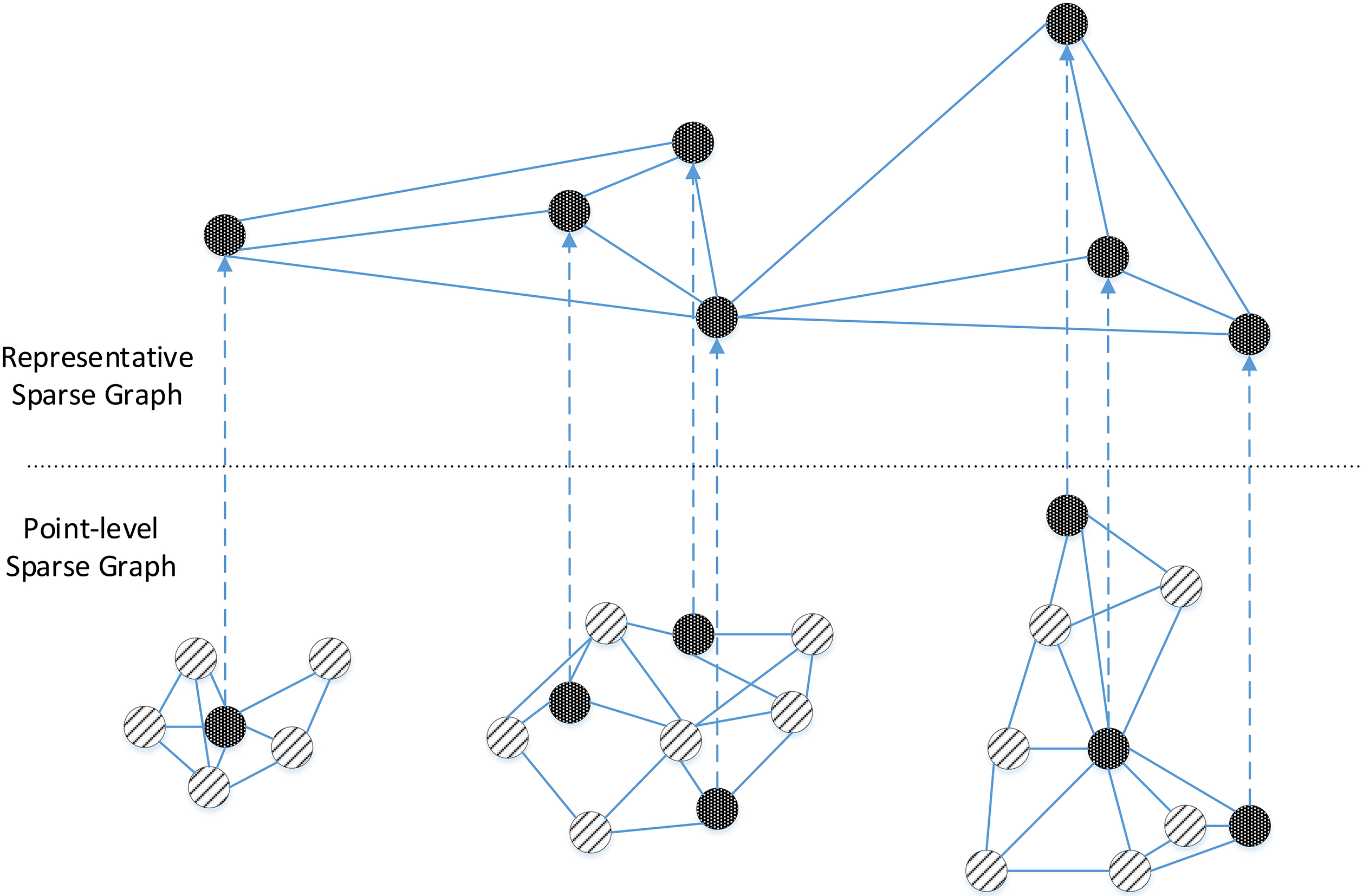
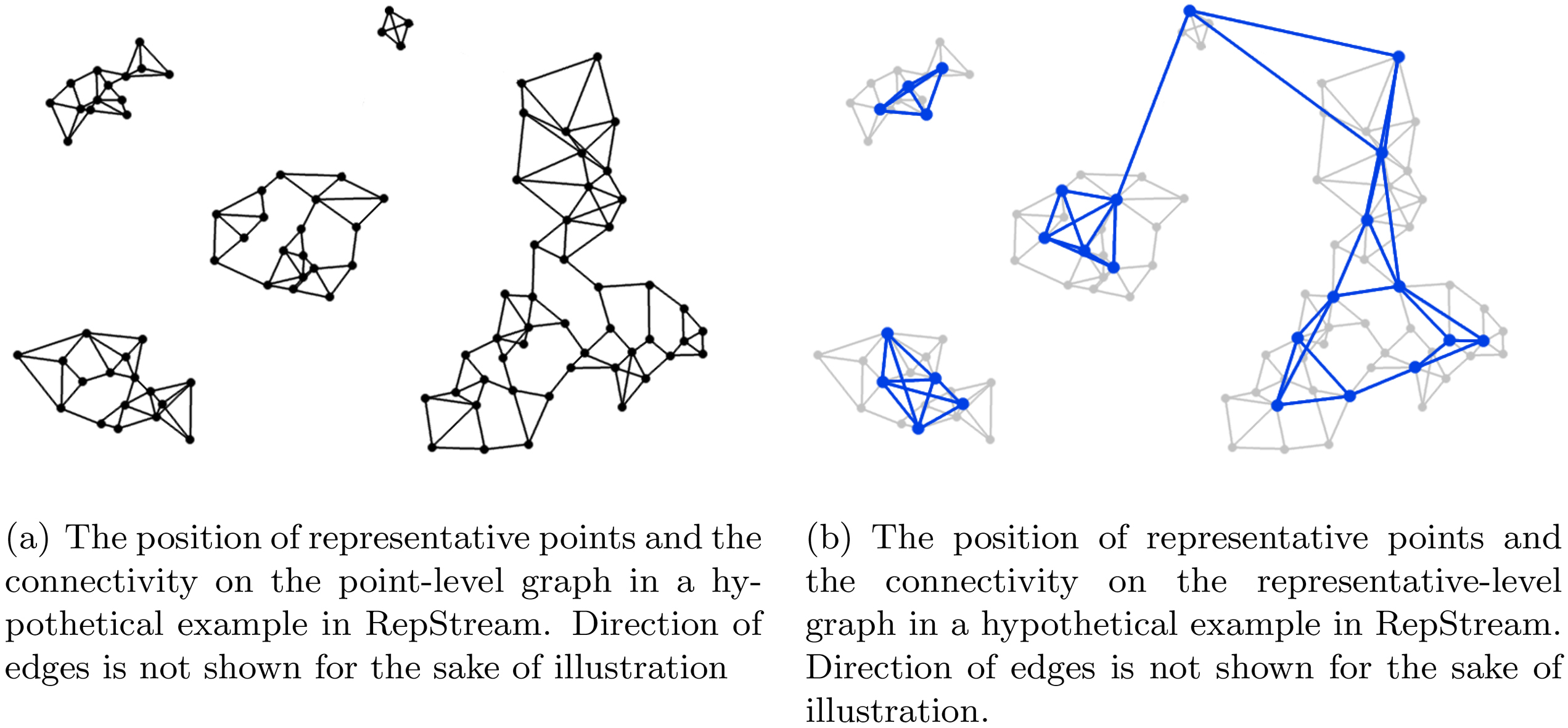
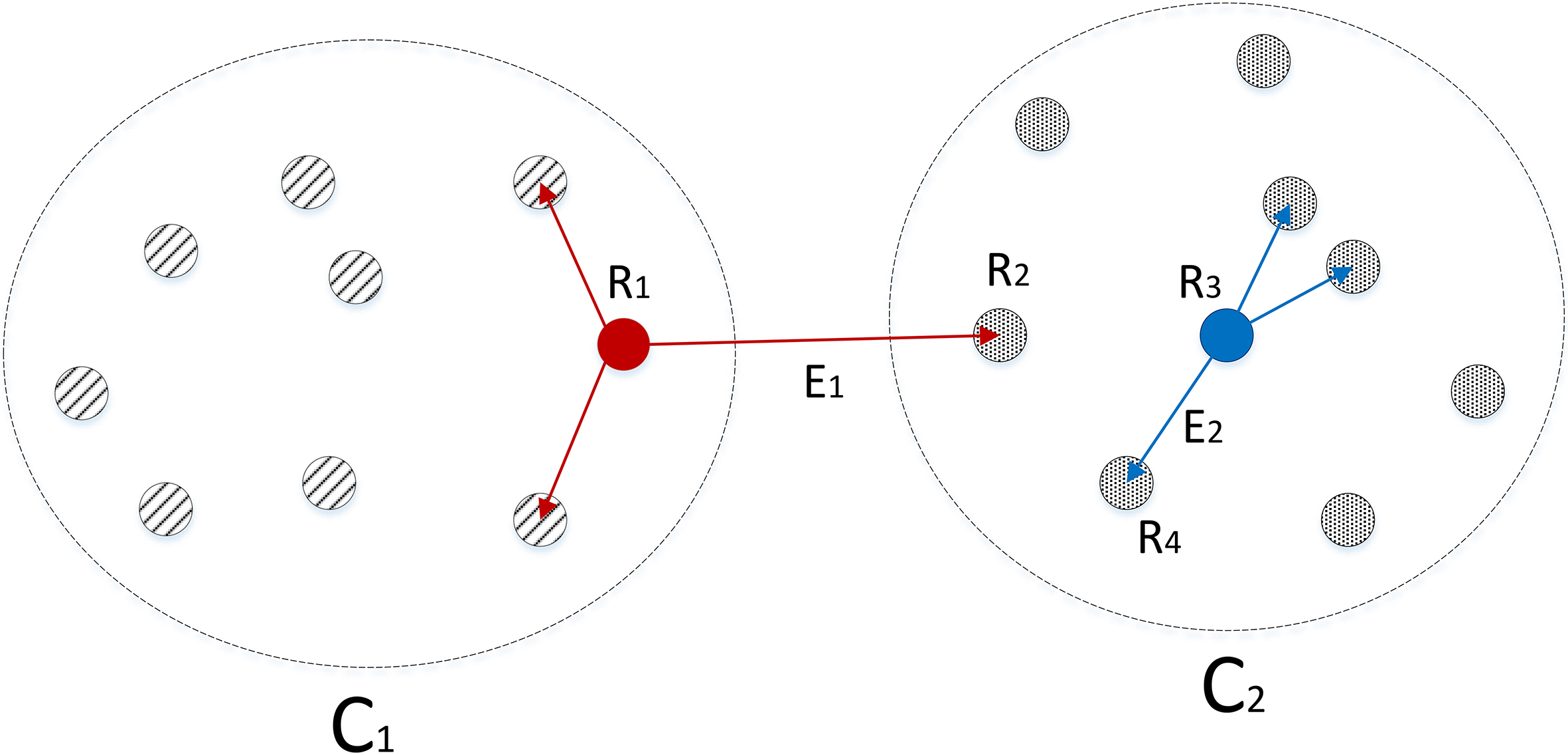
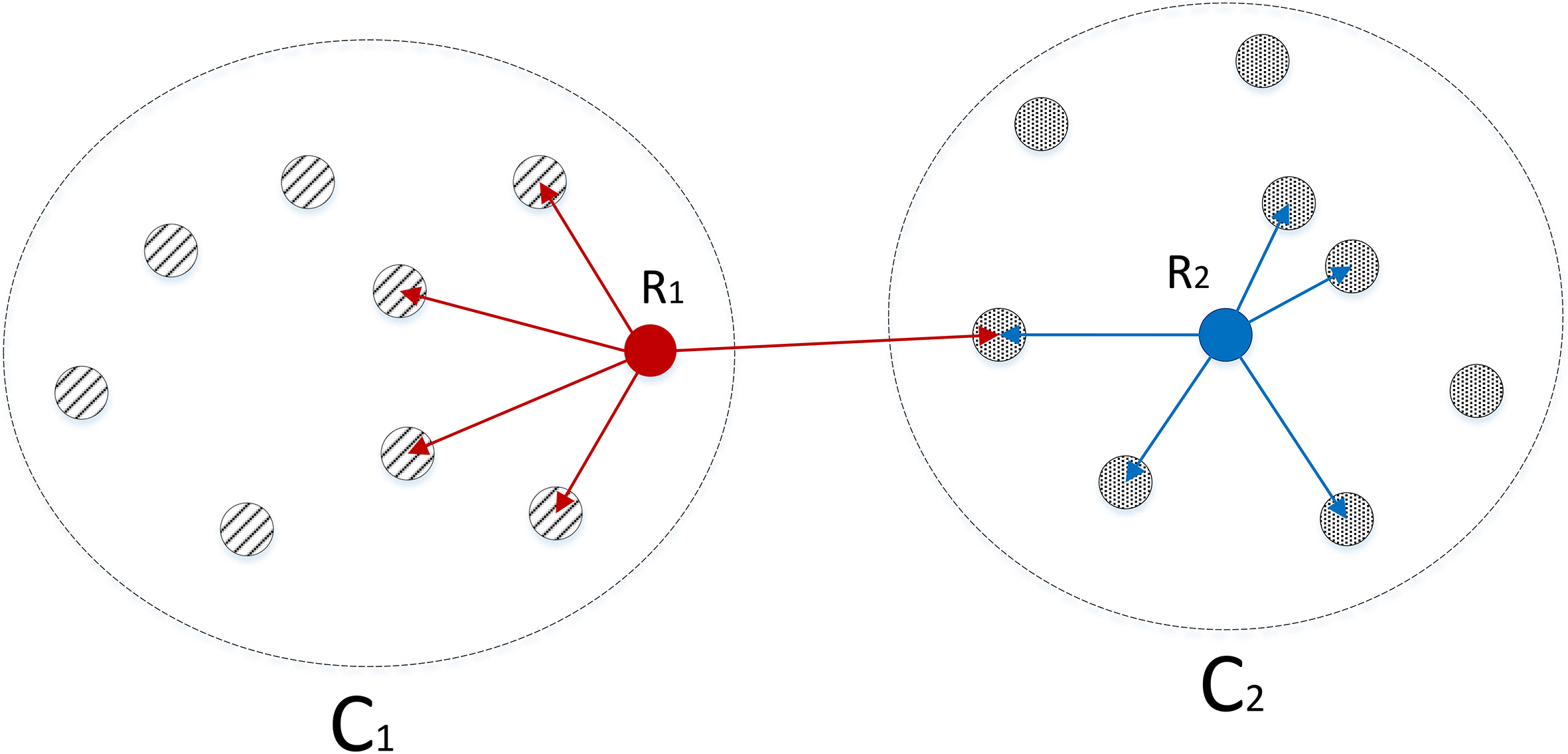
The representative level graph is also a $K$ -NN graph but its vertices consist of only representative points, which are a subset of data points currently kept in memory. A vertex which is newly inserted into the point-level $K$ -NN graph will become a representative point if it has no outgoing edge connecting it to another representative point. This allows representative points to be spread more or less evenly through the data distribution. In this manner representative points are added incrementally as vertices are added to the point-level nearest neighbour graph when no neighbour representative is available. This representative-level graph is where clustering decisions are made. Figure 1 shows the relation between the point-level sparse graph and the representative-level sparse graph, in which a subset of data points are used to construct a second sparse graph on which clustering is performed. Figure 2b shows an example of the representative points and the representative-level $K$ -NN graph in a hypothetical with the corresponding point level graph in lighter grey. Representative points are added incrementally as the stream progresses, this means that as vertices are added to the point-level graph new representative points may be created, and so the representative level graph must be updated incrementally as well.

Figure 1.

An illustration of the representative and point-level sparse graphs in the RepStream algorithm.

Figure 2.

The point and representative level sparse graphs of RepStream.

Figure 3.

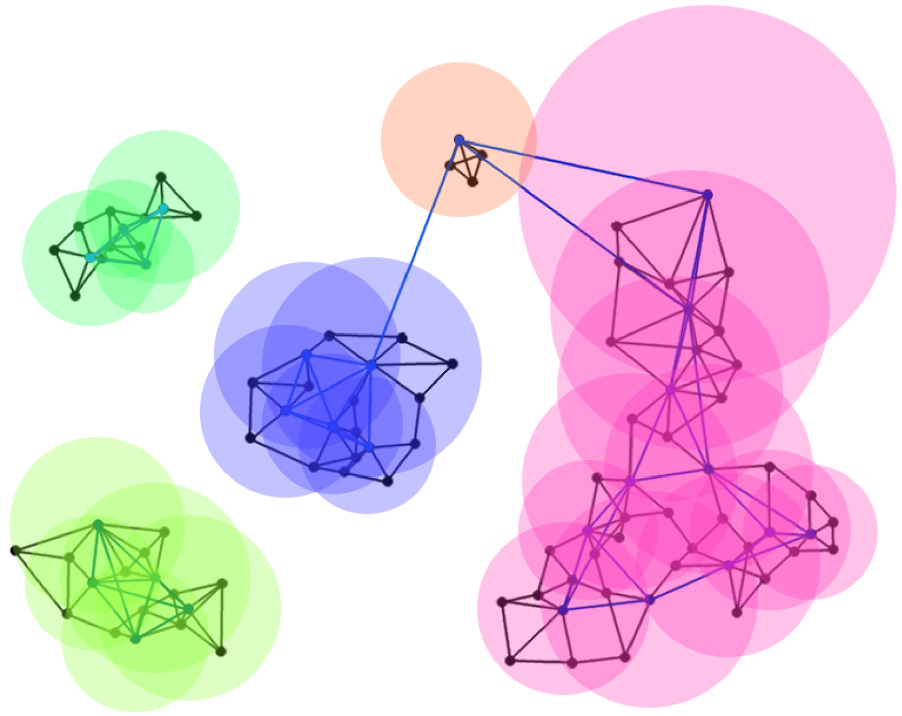
Density relation radii for the representative points in the hypothetical example in RepStream. The distance to the neighbours at the point level determines the density relation radius for the representative level clustering.

3.1.3 The connectivity parameter

K

Repstream’s primary parameter is the graph connectivity parameter $K$ which determines the number of outgoing edges each vertex in the $K$ -NN directed sparse graph structures. This affects the connectivity of data points in memory, and is the primary parameter in determining the final clustering output. A higher $K$ value causes the data points to be more connected, resulting in fewer but larger clusters, while a lower $K$ value causes clusters to be more fragmented due to lower graph connectivity. Because of this, using a value of $K$ appropriate for the data set is important for achieving high quality clustering results, and selecting $K$ appropriately is vital for achieving satisfactory clustering results. There are other parameter values used by RepStream as well, specifically the $\lambda$ decay factor, the $\alpha$ scaling factor. The $\lambda$ decay factor determines how quickly representative points in RepStream are removed over time. The $\alpha$ scaling factor is used in determining when nearby representative points will be placed into the same cluster. The higher the $\alpha$ value, the farther away two mutually connected vertices may be from each other before they are merged, as we explain later in this section. The $\lambda$ and $\alpha$ values are important to RepStream’s operation, however the algorithm is less sensitive to their values, and thus they are easier to set.

3.2 Clustering with density relation

Because of its combination graph and density based approach, users do not need to specify a number of clusters to be found, or assume that clusters must be hyper-spherical. RepStream is able to determine the number of clusters based on its internal graph model, and can find arbitrarily shaped clusters. Clusters in RepStream are made between representative points which are reciprocally connected at the representative level and also density related. Two representative points, and the points that they represent, will be assigned to the same cluster if both these criteria are met.

Reciprocal connections occur when a vertex $v_{i}$ has an outgoing edge to another vertex $v_{j}$ , and the vertex $v_{j}$ has its own outgoing edge to $v_{i}$ . In this case the vertices $v_{i}$ and $v_{j}$ are said to be reciprocally connected. In RepStream reciprocal connections are most important at the representative layer, with reciprocal connectivity between representative points being one of the two criteria to be merged into the same cluster. The other criteria is density relation, as shown in Fig. 3.

Density relation is a concept in RepStream which is determined by the relative distance of nearby points. Two representative points are said to be density related if they are within each other’s density radius. The density radius for a vertex is calculated by taking the mean distance of the vertex’s outgoing edges at the point level, multiplied by the $\alpha$ scaling factor. Two vertices must be within each other’s density radius for them to be density related.

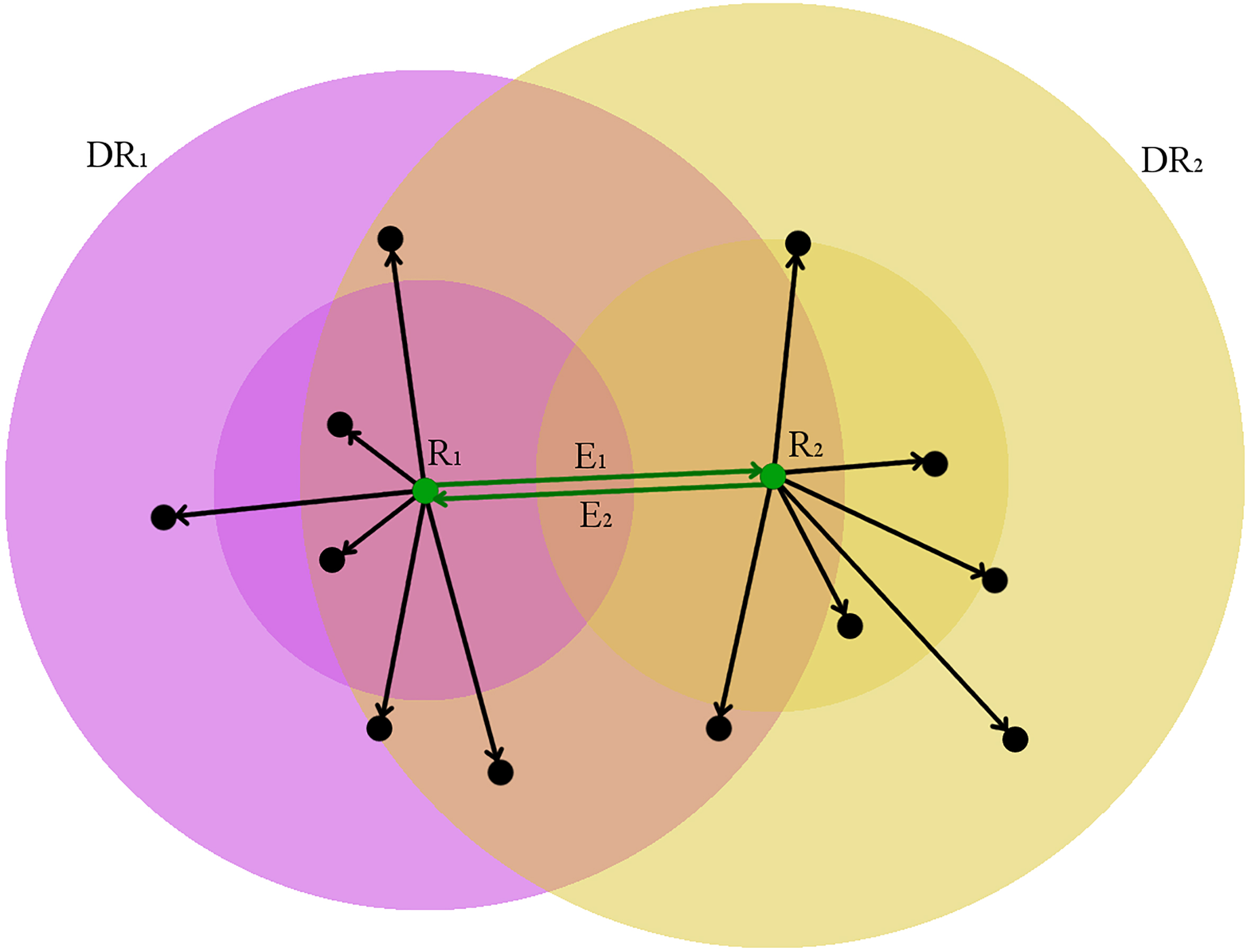
When two representative vertices are reciprocally connected and density related they are merged into the same cluster. Figure 4 shows an example of two representative vertices $R_{1}$ and $R_{2}$ which are reciprocally connected, and are also density related. The vertex $R_{1}$ is within the density radius of $R_{2}$ , and $R_{2}$ is inside the density radius of $R_{1}$ . In this case they would belong to the same cluster, and all nearby point-level vertices they represent would belong to the cluster as well. If a representative point is not reciprocally connected and density related to any other representative points then it will belong to its own cluster. All vertices which are not representative points will belong to the same cluster as their nearest representative vertex, thus all points in the data set will belong to an existing cluster at all times.

A chain of reciprocally connected and density related vertices can cause large clusters to form. This state can change as new data points are added and older data points are discarded. When representative points which were previously in the same cluster lose their reciprocal connection, or lose their mutual density relation then RepStream checks whether the cluster needs to be split. Similarly, existing representative points which belong to different clusters can merge together if newly added points cause them to meet the reciprocal connection and density relation criteria with a representative point belonging to another cluster.

Figure 4.

The representative vertex $R_{1}$ and $R_{2}$ share a reciprocal connection at the representative level, and are also density related. The density radius of the vertices is shown as $DR_{1}$ and $DR_{2}$ respectively, which is the average distance to neighbours at the point level, multiplied by the alpha scaling factor.

4. Proposed method

As can be seen, the performance of RepStream depends largely on how well the connectivity parameter $K$ is specified by the input. The value of this input parameter is significantly influenced by the statistics of the underlying data: it will over-cluster data points if $K$ is too small, and under-cluster data points if $K$ is too large. Unfortunately, RepStream does not have the ability to tell which $K$ value is appropriate and hence relies totally on the user’s input, much like many other $K$ -NN-based clustering algorithms.

To address the limitation of RepStream, we study the distribution of edge lengths over the $K$ -NN graphs and how it depends on the connectivity parameter $K$ . We follow the fundamental principle in machine learning, which is to select the simplest model that explains the data well. Here, the model complexity is inversely proportional to $K$ as described above, and the explain-ability of the model is, according to our definition, how well the distribution of the normalised edge lengths still looks ‘normal’. By searching for the simplest model that still controls the deviation of the normalised edge length distribution under a pre-defined level, we can automatically adjust clustering outputs when the underlying data statistics changes. Based on the RepStream algorithm, our proposed RobustRepstream consists of two main parts:

•
The computation of the skewness excess score of the distribution of normalised edge lengths at each vertex.
•
Automatic model selection based on the computed skewness excess score.

4.1 Skewness excess

To motivate our approach, we start with an intuition shown in Fig. 6. Typically, in a volume of even distribution of data points the edges will be more likely to be spread evenly in all directions. A data point in the middle of a class has other vertices belonging to that class all around it, and so the variation in edge length of its neighbours will be relatively small. In the middle of a cluster there are data points in all directions, so there are likely to be more available neighbours at relatively even distances. In this example, the vertex $R_{2}$ is near the centre of the class $C_{2}$ and so many intra-class edges can be made, even if the connectivity of $R_{2}$ is increased. On the other hand the vertex $R_{1}$ is near the edge of the class, and so the potential intra-class neighbours is fewer. There are limited directions in which nearby intra-class edges can be made, and the other directions border the areas of low density which, as we discussed before, separates clusters. Any inter-class edge must traverse this distance, as in Fig. 5, which means the edge length will likely be longer than inter-class edges. Vertices on the edge of a cluster are therefore more likely to have longer, less consistent edge lengths for neighbours.

Suppose that desirable clusters are regions of contiguous (but not necessarily convex) space which are populated by data points in a more or less similar distribution. These regions we assume are separated either by significant regions of empty space, or by data points at a significantly lower density than inside the clusters. From this assumption, it follows that data points near the edges (but still inside) a cluster are very likely to have the first few of their nearest neighbours belonging to the same cluster, and that the chance of the next nearest neighbour belonging to a different class (an inter-class neighbour) increases as the number of nearest neighbours being considered increases. This means the connectivity needs to be adjusted to reflect the desirable clustering outcome.

Figure 5.

Intra and Inter-class edges. The Edge $E_{1}$ is considered an inter-class edge as it connects two vertices $R_{1}$ and $R_{2}$ that belong to different ground-truth classes. Edge $E_{2}$ connects two vertices belonging to the same class and thus is considered an intra-class edge.

Figure 6.

An illustration of relative edge lengths of nearest neighbours in the middle of a cluster versus near the edge of a cluster.

As can be seen, once all the nearby vertices within a multi-dimensional sphere have been connected to, additional neighbours will have a greater and greater likelihood of being significantly further away than existing neighbours. It is these longer than average edges which the score is intended to reflect, and high numbers of large edges suggest that the number of edges has grown too large. They are more likely to be on the long tail of the distribution of edge lengths. Note that as the edge lengths are non-negative, the more extreme values of edge lengths associated with a vertex, the more skew to the right the distribution of the edge lengths. Therefore, the excess at the right tail of the distribution of the edge lengths captures the presence of these large values. Based on this intuition, we introduce a novel concept of skewness excess.

In what follows, we denote as $v_{i}$ the vertex $i$ of interest, $e_{i,j}$ as an outgoing edge from vertex $v_{i}$ to another vertex in its neighbourhood $\mathcal{N}_{K_{i}}({v_{i}})$ . We also denote as $X_{e_{i,j}}$ the normalised length of the edge $e_{i,j}$ . Here, normalisation is performed with respect to the distribution of original outgoing edges from vertex $v_{j}$

$\displaystyle X_{e_{i,j}}=\frac{l_{e_{i,j}}}{1.4826\nu_{i}},$ (1)

where $l_{e_{i,j}}$ is the original length of the edge $e_{i,j}$ and $\nu_{j}$ is the median of the absolute deviation (MAD) of the $K$ values of $l_{e_{i,j}}$ . The reason we use $1.4826\nu_{i}$ is because it is a robust measure of the deviation of the edge lengths [29]. Given that a vertex may have a relatively small number of outgoing edges – fewer than 10 – the standard deviation is not a reliable measure.

To capture the tail behaviour of the edge length distribution, we define the thresholding function

.

The thresholding function $\rho_{\tau}(x)$ with a threshold $\tau$ is defined as

$\displaystyle\rho_{\tau}=\left\{\begin{array}[]{ll}x&\mbox{if }x>\tau,\\ 0&\mbox{if }x\leqslant\tau.\end{array}\right.$ (2)

Denote as $\bar{X}_{v_{i}}$ the median of all normalised edge lengths associated with $v_{i}$ . We formally introduce the following concept

.

The skewness excess score (SE) of $K_{i}$ normalised edge lengths associated with a vertex $v_{i}$ is

$\displaystyle SE(v_{i})=\sum_{e_{ij}\in\mathcal{N}_{K_{i}}({v_{i}})}\rho_{1}(X% _{e_{i,j}}-\bar{X}_{v_{i}})$ (3)

Note that the subscript $i$ in $K_{i}$ indicates that $K_{i}$ is locally specific to each vertex, as opposed to a single global $K$ in RepStream and most $K$ -NN data stream clustering algorithms. Here, the skewness comes from the older notion of nonparametric skew, and the excess is due to our choice of considering only edges with normalised length greater than the median by 1. Edges that exceed this length will be considered in the overall skewness score. Consequently, additional neighbours must be within a relatively limited distance of existing neighbours, otherwise the edge will be considered anomalous. As the number of outgoing edges, and neighbours therefore get farther and farther away, the total skewness excess tends to increase as shown in Fig. 9.

Figure 7.

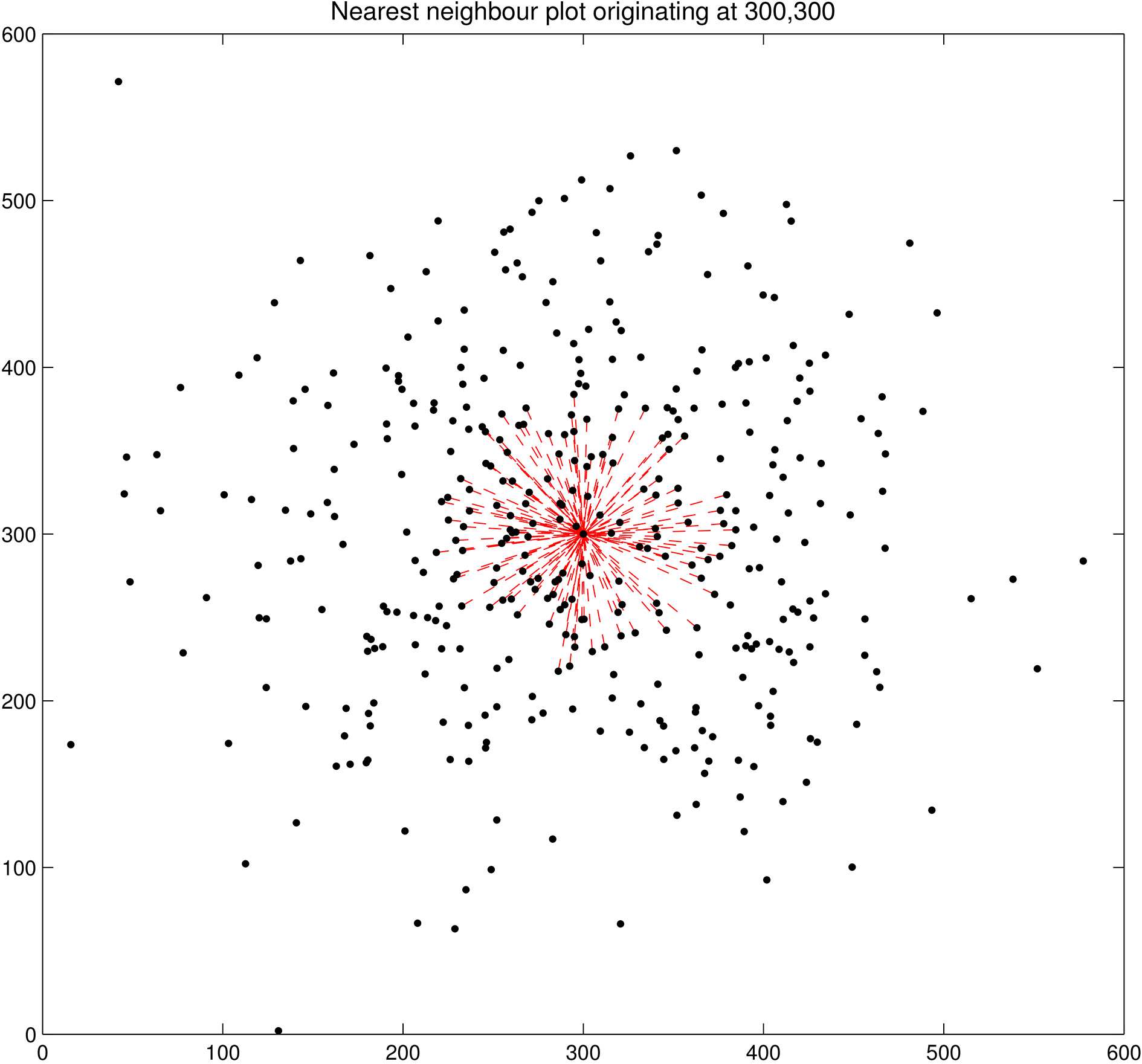
Nearest neighbour plot of a 400 point 2 dimensional normal distribution with a standard deviation of 100. Plot shows the 200 nearest neighbours from the centre of the distribution.

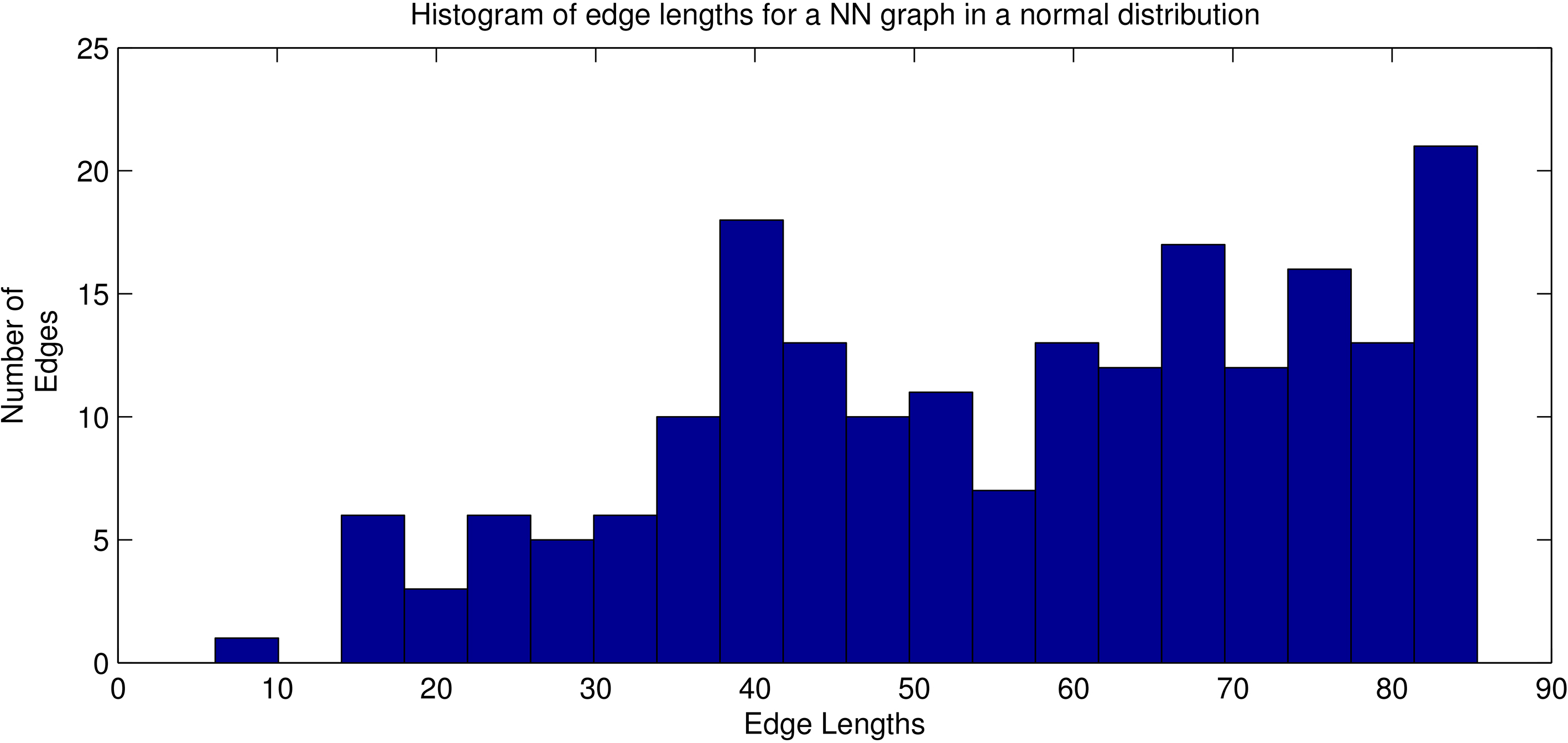
Given that the area of a hyper-sphere increases exponentially as the radius is increased, the variance in edge length of additional neighbours should decrease. Figure 7 shows an example of the 200 nearest neighbours of a vertex in a 2 dimensional normal random distribution consisting of 400 vertices in total in which the standard deviation is 100. Figure 10 shows a histogram of the length of the edges to these nearest neighbours.

This example follows our expected trend, in which the distribution of edge length is weighted towards the far end. With this knowledge we expect a vertex in the middle of a cluster will have a more concentrated distribution, whereas a vertex near the edge of a cluster will have a more right-tailed distribution. This is the key principle of our proposed RobustRepStream.

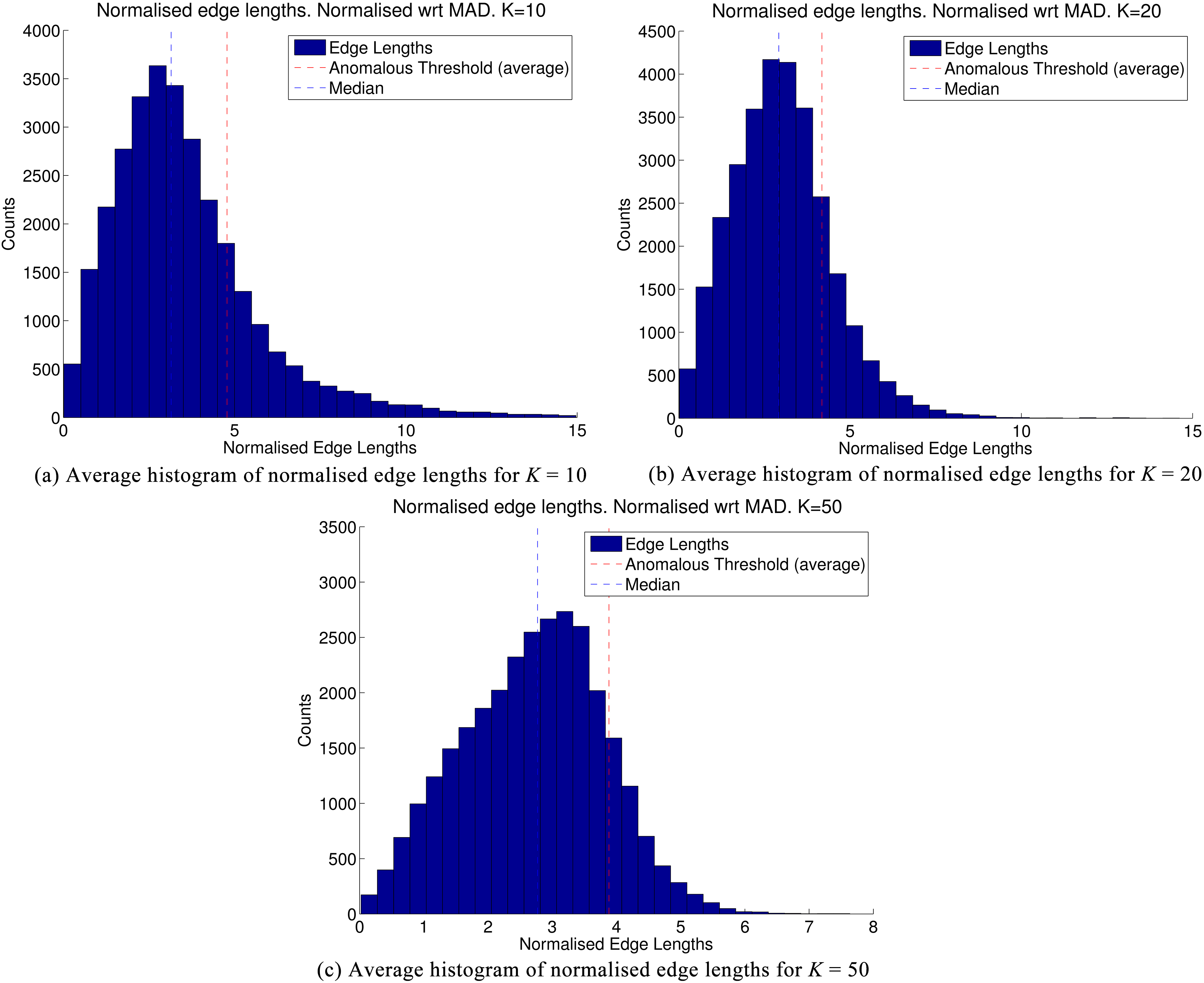
Next, we briefly study the asymptotic behaviour of the skewness excess score through a real example when both $K$ and the number of vertices are sufficiently large. We sample 2-dimensional data from a uniformly random distribution, and define a point directly in the centre of this distribution as our evaluation point, and run our proposed method. At a point in the middle of the stream, we examine the average of the distributions of the normalised edge lengths for two different values of $K$ (Fig. 8a–c) as well as the average skewness excess score calculated over all vertices (Fig. 9). Here, we make two interesting observations. The first observation is that the average distribution exhibits a linear behaviour for edge length below the median, and exponential decay beyond the median for both $K=20$ and $K=50$ . The tail behaviour is also consistent with our intuition: when $K=10$ (small), there are relatively more large values at the tail as the model is more ‘complex’ and tends to produce smaller clusters with less data points. Consequently, a large edge length will be more likely to be anomalous compared to the rest. When $K=50$ , it is less likely for an edge to be relatively large compared to the rest, and therefore the distribution is more concentrated around the median.

Figure 8.

Normalised edge lengths for various $K$ values.

Figure 9.

Average SE vs $K$ , normalised with respect to MAD.

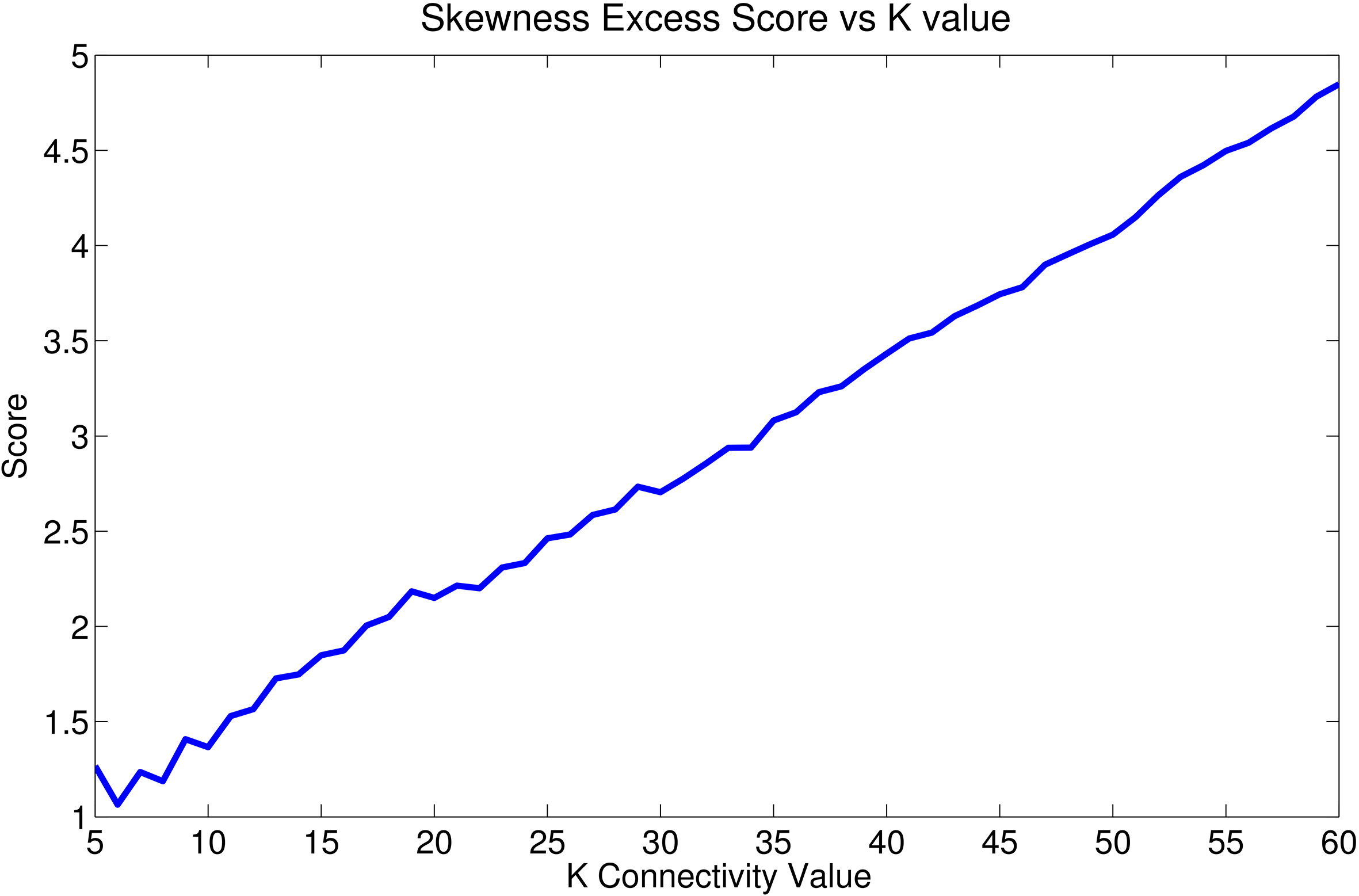
The second observation is that the average skewness excess score exhibits an approximately linear relationship with respect to $K$ over the practically meaningful range of values for $K$ . This is also consistent with our intuition, because on average the term in the sum converges to the first-order moment of the distribution of the normalised edge lengths partially over the support beyond $1+\nu_{i}$ , and the fact that there are $K$ terms in the sum. This linear asymptotic behaviour is important because it allows us to provide a trade-off between model complexity and data explain-ability more easily: the larger the $K$ , the less complex the model (less clusters), but the more discrepancy with data statistics (more inter-class pairs in a cluster). Due to the linear relationship, a one-dimensional search for the optimal value of $K$ will be feasible without a risk of facing multiple local optimum values, at least in the asymptotic sense. This is what we propose do exploit next.

Figure 10.

Histogram showing the distance to the nearest 200 vertices in a 400 point 2 dimensional normal distribution, with the origin at the centre of the distribution. Standard deviation is 100 in both the x and y direction.

4.2 RobustRepStream

The RobustRepStream algorithm is an extension of the RepStream algorithm detailed in the previous section. RobustRepStream, uses a completely distinct method for selecting outgoing edges for each vertex, at both the point and representative levels. The skewness excess score as described previously is used to determine how many edges each vertex should have when it is inserted into the graph. In the original RepStream algorithm, every vertex will always have the same number of edges connecting to other vertices, regardless of the relative distance to the farther neighbours compared to closer neighbours. Not only must a user correctly select a single $K$ value for use during an entire stream’s length, but the inflexibility in neighbour counts means one must make the trade-off between over-clustering and under-clustering. To address this limitation, we aim to achieve two goals with the proposed algorithm:

Goal 1: Remove the need for the user to set the sensitive $K$ parameter at runtime. As we have mentioned in previous sections, initial parameter selection is a challenge, and our method aims to converge towards a desirable clustering solution. Goal 2: Allow vertices in the two NN graphs to have dynamic and different levels of connectivity as is appropriate for their local region. Setting outgoing edges in a dynamic manner allows the construction of a nearest neighbour graph which takes the context and distances of the nearest neighbours into account. Allowing vertices in the nearest neighbour graph to have different numbers of outgoing edges will give us the potential to allow different levels of connectivity in denser regions of data, compared to uneven or sparse regions.

The RobustRepStream works on the principle of balancing between model complexity and data explain-ability and it proceeds as follows. For any newly inserted vertex $v_{i}$ we aim to find an optimal value of the $K_{i}$ connectivity parameter locally specific to the vertex. To so do, we do a one-dimensional search, which starts from a pre-defined value $K_{i}=K_{i}^{\min}$ and gradually increases it. At every possible value of $K_{i}$ , we examine the skewness excess score of the distribution of the $K_{i}$ normalised edge lengths associated with $v_{i}$ . The selected $K_{i}$ is then the maximum value at which the skewness excess score is still below a universal threshold $\alpha$ describing the maximum discrepancy between what the model assumes and the actual data

$\displaystyle K_{i}=\arg\max_{K>K_{i}^{\min}}SE(v_{i})\leqslant\alpha.$ (4)

The result of this is that each vertex will have the maximum number of neighbours possible, whilst still remaining under the skewness excess score threshold. When a vertex is added or removed, nearby vertices must also be adjusted by either adding or removing outgoing edges until the number of edges is the highest possible while remaining below the maximum allowable threshold.

Compared to the original RepStream algorithm and many other $K$ -NN-based clustering methods, RobustRepstream has removed the global connectivity parameter $K$ . Whilst our proposed algorithm has introduced the new threshold $\alpha$ , it is much less sensitive to the data unlike the connectivity parameter, which is clearly demonstrated in the sensitivity analysis we show later. Because it is based on the distribution of the normalised edge lenghths, it is invariant to the scale of the data. It is purely a subjective definition of what an acceptable level of excess skewness by the user. In fact, a universal value $\alpha=2$ is recommended for all data sets. The proposed RobustRepstream method consists of two algorithms:

•

The first algorithm determines the number of outgoing edges for a newly added vertex as shown in Algorithm 4.2. In this algorithm, the inputs are vertex, the new vertex, minEdges the minimum number of edges a vertex must have, and $\alpha$ is the density existing scaling factor parameter used by RepStream. The function $\textit{GetNextNeighbour}(\textit{vertex})$ gets the closest neighbour that the vertex does not already have an edge to, and the function $\textit{CreateEdge}(\textit{vertex},\textit{newNeighbour})$ creates an outgoing edge from vertex to newNeighbour.

[h] f Algorithm for determining the outgoing edges for a newly added vertex. $\textit{FUNCTION}:\textit{AddEdges}$ $\textit{INPUT}:\textit{vertex},\textit{minEdges},\alpha$ $\textit{vertex.neighbours.count}<\textit{minEdges}$ $\textit{newNeighbour}\leftarrow\textit{GetNextNeighbour}(\textit{vertex})$ $\textit{CreateEdge}(\textit{vertex},\textit{newNeighbour})$

$\textit{newNeighbour}\leftarrow\textit{getNextNeighbour}$ $\textit{SkewnessExcessScore}(\textit{vertex},\textit{newNeighbour})<\alpha$ $\textit{CreateEdge}(\textit{vertex},\textit{newNeighbour})$ $\textit{newNeighbour}\leftarrow\textit{getNextNeighbour}$

•

The second algorithm calculates the skewness excess score if the vertex newNeighbour were to hypothetically become a neighbour, and is shown in Algorithm 4.2. In this algorithm, the average and median absolute deviation values are calculate as avg and dev respectively with the potential new edge, then the edge anomaly score for the potential edge is computed and returned. The function $\textit{SumDistances}(\textit{vertex.neighbours})$ finds the sum of the distances to all existing neighbours, while the function $\textit{Distance}(\textit{vertex},\textit{neighbour})$ finds the distance between two vertices.

[h] Algorithm for calculating the skewness excess score of a vertex if a potential new neighbour were to be added. $\textit{FUNCTION}:\textit{SkewnessExcessScore}$ $\textit{INPUT}:\textit{vertex},\textit{newNeighbour}$ $\textit{score}\leftarrow 0$ $\textit{dev}\leftarrow 0$ $\textit{PotentialNeighbours}\leftarrow\{\}$ $\textit{PotentialNeighbours}\leftarrow\textit{vertex.neighbours}+\textit{newNeighbour}$ $\textit{avg}\leftarrow\textit{Median}(\textit{PotentialNeighbours.distances})$

$\textit{AbsDevs}\leftarrow\{\}$ neighbour in PotentialNeighbours $\textit{AbsDevs.add}(|\textit{Distance}(\textit{vertex},\textit{neighbour})-% \textit{avg}|)$

$\textit{dev}\leftarrow 1.4826\times\textit{Median}(\textit{AbsDevs})$

neighbour in vertex.neighbours $s\leftarrow 0$ $\textit{Distance}(\textit{vertex},\textit{neighbour})-\textit{avg}>\textit{dev}$ $s\leftarrow(\textit{Distance}(\textit{vertex},\textit{neighbour})-\textit{avg}% )\div\textit{dev}$ $\textit{score}\leftarrow\textit{score}+s$

$\textit{Distance}(\textit{vertex},\textit{newNeighbour})-\textit{avg}>\textit{dev}$ $s\leftarrow(\textit{Distance}(\textit{vertex},\textit{newNeighbour})-\textit{% avg})\div\textit{dev}$ $\textit{score}\leftarrow\textit{score}+s$

score

Once a suitable number of outgoing edges is found so that the skewness excess is below the threshold $\alpha$ , RobustRepStream assigns clusters using the same mechanism as the original RepStream algorithm.

The existing $\alpha$ parameter is used due to its existing usage in RepStream for determining density relation, as described in the previous section. The density relation radius is equal to the average length of the vertex’s nearest neighbours multiplied by the $\alpha$ parameter, and defines an upper limit to the distance between representative points for them to be merged into the same cluster. Our skewness excess threshold follows a similar concept, being an upper-limit to the relative length of edges to nearest neighbours.

As is similar to its original usage in RepStream, $\alpha$ is a relatively insensitive parameter which is much easier to set than the $K$ value. Intuitively, an alpha value of $\alpha\leqslant 1$ makes little sense since representative vertices are only created when a vertex has no reciprocal link to an existing representative, and so representative vertices are most likely to be spread out. Skewness excess threshold values less than 1 also make little sense because the edge score cannot have a value between 0 and 1.

We found empirically that the universal choice $\alpha=2$ works well across many types of data streams. We also define a lower bound to the number of edges as being $\textit{minEdges}=6$ , as fewer edges than this makes the computation of median absolute deviation less meaningful. This is what we use in our experiments in Section 5, regardless of data set. An $\alpha$ value of 2 allows vertices to have no more than 1 anomalous edge, as the minimum excess score of an anomalous edge is 1.

5. Experiments

To evaluate RobustRepStream we perform experiments on a number of real-world and synthetic data sets. These datasets are specifically selected to be examples of streaming data which evolves over time, exhibiting concept drift with which we can evaluate our RobustRepStream method.

5.1 Real world data sets: KDD and Tree Cover

5.1.1 The KDD Cup 1999 data set

The KDD’99 data set [20] is a well-known benchmark data set. It is extracted from logs taken from a smart firewall in a network being subjected to simulated and controlled network attacks. It contains high dimensional data, of which we use the 34 numerical features with each data point presented as a 34-dimensional vector. We use a subsampled version of the data set containing 494 020 datapoints, which is about 10% of the original KDD Cup 1999 data set. Most of the data in the subsampled data set we used for evaluation falls into either the normal traffic class, or one of two major denial-of-service attack classes. A relatively small percentage of the data – less than 2% – are from 20 other network attack types. Each data point is labelled with the type of traffic (normal, or the type of attack) for evaluation purposes.

This KDD Cup 1999 data set has been used previously in evaluating stream clustering algorithms [1, 2, 6, 23] due to the high variability between classes in the data set. The various network attacks interrupting the normal traffic represent changes in the distribution of subsequent data points, known as concept drift. This is a significant challenge for clustering algorithms to deal with, making it an excellent data set for testing how an algorithm deals with dynamic, unpredictable data point distributions over time.

5.1.2 The Tree Cover Type data set

The CoverType data set [7] is a real-world data stream of a set of features extracted from satellite photos and geological surveys from forested areas of northern Colorado. It contains over 580,000 entries with ground truth labels corresponding to which type of trees grow in each area, and has been previously used as a benchmark data set for stream clustering [23, 6, 13]. This data represents a naturally evolving stream of data which changes with the environment and climate of each region. As such, this data set, as well as the previous KDD data set, both contain real-world examples of concept drift in a streaming context. The dataset has 10 dimensions which include quantitative measures of elevation, aspect, slope, distance from water source, distance from roadway, and level of incident sunlight. Whilst this stream evolves over physical location rather than over time, it is still effective for use as a benchmark dataset exhibiting concept drift. Both this data set and the KDD dataset contain a level of natural noise due to their respective collection methods

5.2 Synthetic data sets

The synthetic data sets we present here are designed to evaluate our algorithm on controlled levels of concept drift, which present specific challenges to the algorithm and demonstrate its ability to handle change over time. As such, these data sets include data sets which require variable levels of connectivity in order to achieve the highest quality clustering results.

5.2.1 Closer data set

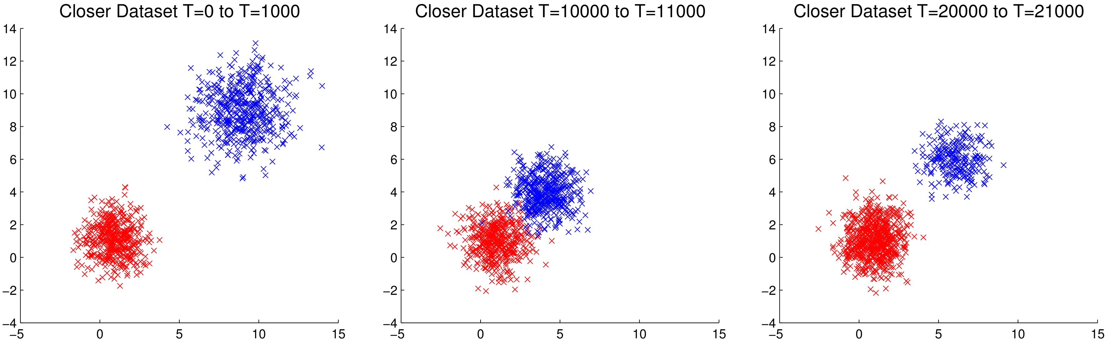
The Closer data set is an evolving data set which has three distinct stages. The first 10,000 data points alternate between two classes, all data points are on a two-dimensional plane and each class is normally distributed with a large level of separation between the two classes. In the second 10,000 data points, the two classes suddenly become much closer together, such that the two classes borders are overlapping. The final 10,000 points have a greater degree of separation once again, however one class becomes more dense, while the other becomes less dense. Figure 11 shows these three stages. The changes in this data set are sudden, being taken from only three different distributions.

Figure 11.

The evolution of the Closer data set, showing slices of its 3 sections.

The three stages of the data set were sampled like so:

•

Between $T=0$ to $T=10,000$ class A was centred at 1,1 and normally distributed with a $\sigma$ of 1 in both the x and y axes. Class B was centred at 8,8 with a $\sigma$ of 1.5 on both axes. Points were sampled from these distributions alternately between classes.

•

Between $T=10,000$ to $T=20,000$ class A remained the same, while class B was moved to 4,4. Points were sampled from these distributions alternately between classes.

•

Between $T=20,000$ to $T=30,000$ class A remained the same, while class B was moved to 6,6 with a $\sigma$ of 1.5 on both axes. Points were sampled from these distributions randomly by alternately selecting 3 points from class A, followed by 1 point from class B.

Figure 12.

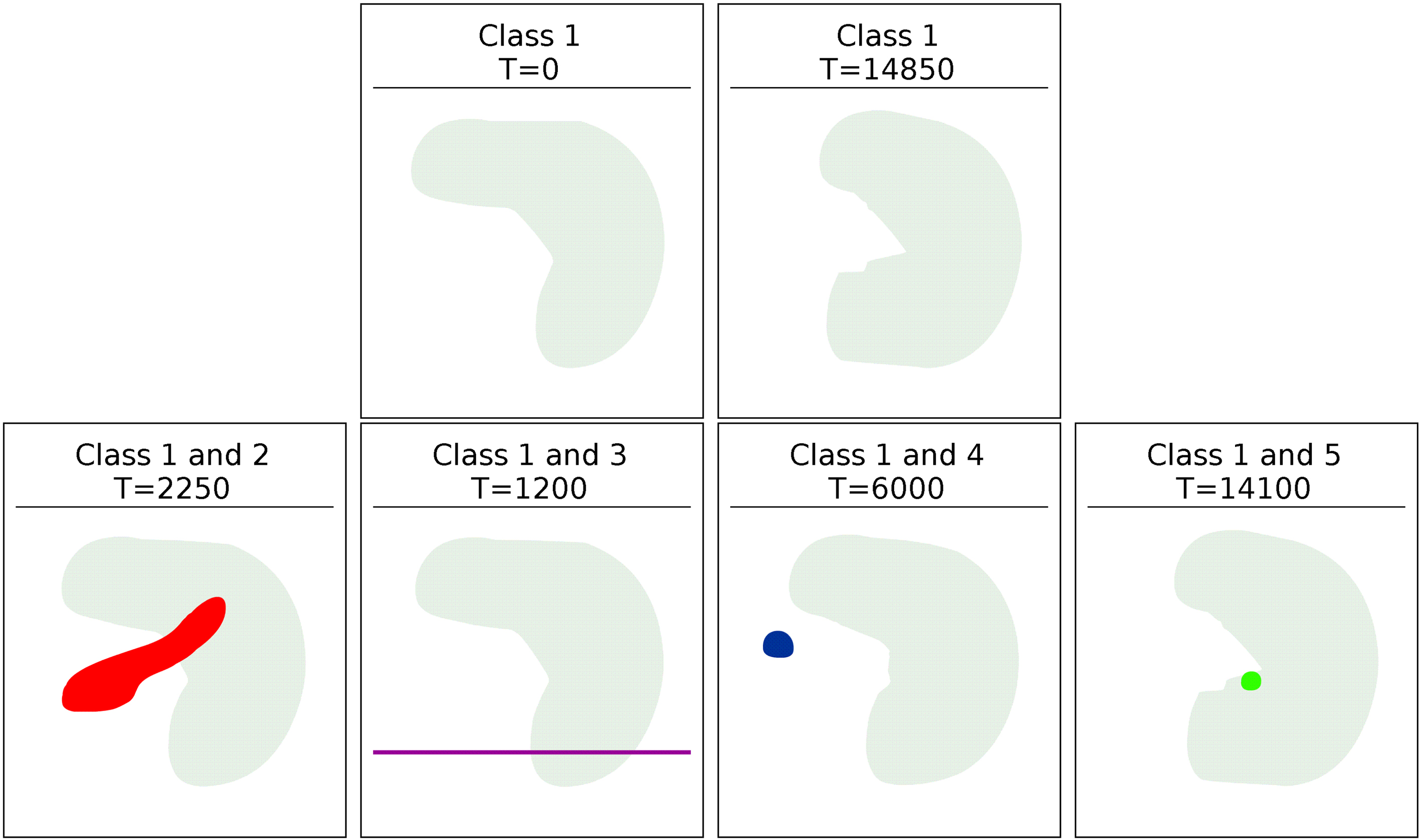
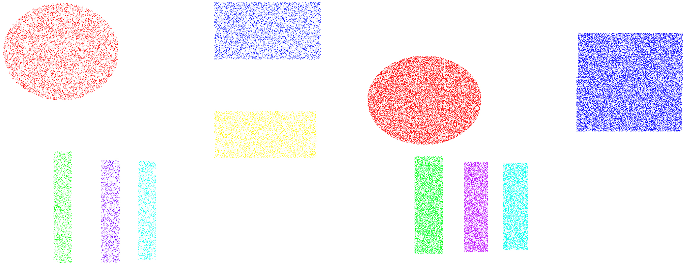
Two dimensional representations of the 5 different classes. The main class is always present and steadily changes shape, the smaller classes appear at various points through the data set, as shown in Fig. 13.

5.2.2 SynTest data set

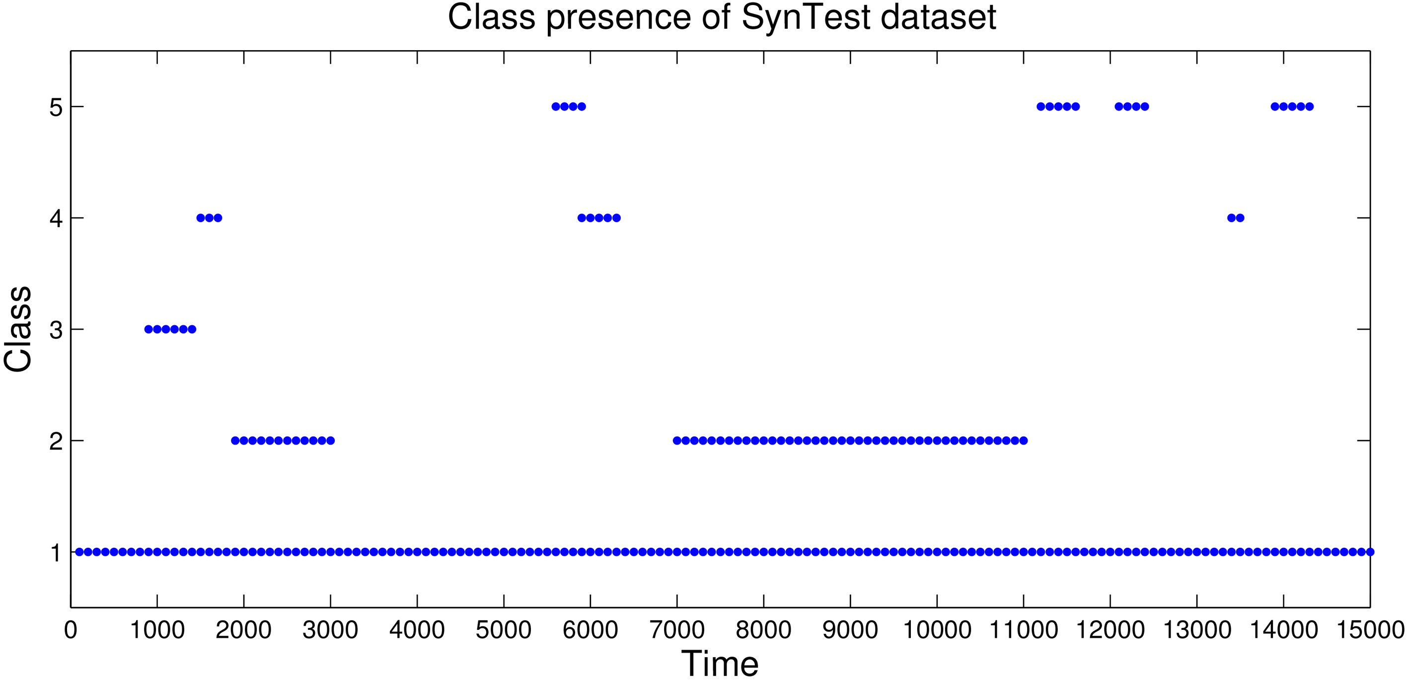
The SynTest data set is also an evolving data set that consists of one large class which slowly shifts its shape and position over time, as well as several other smaller, more dense classes which appear and disappear at various points. The larger class is present throughout the whole data set, and makes up a majority of the data points, the smaller classes exist for a relatively shorter amount of time. Each of these smaller classes are more dense than the main class, but are present for only a few hundred, to a few thousand time-steps at a time.

Figure 13.

The class presence of the classes in the SynTest data set. A marker indicates the class is present in the data set during the given time window.

Figure 13 shows the presence of the classes in the SynTest data set. Marks indicate when the given class is present in the given time window. The shape, size, and position of the classes is shown in Fig. 12. Class 1 is always present through the data set, while the other classes are present for shorter time periods.

5.2.3 Shapes data set

The Shapes data set is an evolving data set split into two distinct stages made from two distributions. In the first stage, shown in Fig. 14, the data set shared amongst 6 classes which are largely separated. In the second stage, the classes are moved closer together, and the two classes on the right of the data set merge to become one larger data set. The transition between these two stages presents a significant challenge to clustering algorithms, as a lower degree of separation between classes makes those classes harder to distinguish. Additionally, the two classes that are merged together means that the algorithm will have to adapt and merge clusters that were previously separated.

Figure 14.

The first and second stage of the Shapes data set.

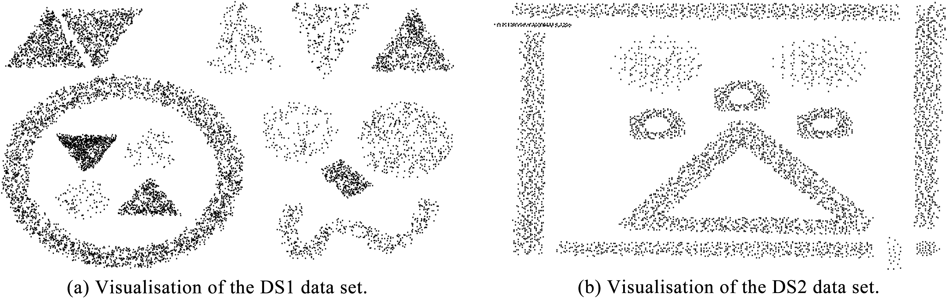
5.2.4 DS1 and DS2

The DS1 and DS2 data sets are data sets made from a static distribution which were used to evaluate the original RepStream algorithm. They are shown in Fig. 15a and b and have no intentional stream evolution over time.

Figure 15.

The DS1 and DS2 datasets.

The DS1 and DS2 data sets are included as static data sets to demonstrate our method’s ability to adapt to a static distribution, and to converge towards a stable clustering solution. The Closer, SynTest, and Shapes synthetic data sets all have specific and very controlled instances of concept drift over the length of the stream. These synthetic evolving data sets are used to demonstrate how our method can adapt to changing data distributions over time.

5.3 Evaluation metrics

Since we have access to the ground truth class labels for the data set we are able to use external validation metrics as a way to determine the accuracy of our clustering methods. External validation metrics are more accurate in measuring the absolute quality of clustering results because they use a comparison to a ground truth. While internal validation metrics can be useful, they make assumptions about the data set which may be inaccurate, for example the sum of squared errors (SSQ) evaluates the compactness of clusters, with a lower score being more desirable. This measure assumes ideal clusters are hyper-spherical in shape, which is not a safe assumption, since clusters can be arbitrarily shaped.

We use the average $F$ measure score of clusters compared to the ground truth over the length of the data set as a method of measuring the performance of our RobustRepStream method against the base RepStream algorithm. We choose the external validation metric, $F$ measure since it can be used to compare clustering results, while penalising both different ground-truth classes being mixed into the same cluster, and also single classes being fractured into multiple clusters. The commonly used purity measure is more popular for evaluation, but has a problem in that it does not penalise classes being fractured into sub-clusters [21]. For this reason we find $F$ measure to be a more accurate representation of cluster accuracy than the more popular purity measure for evaluating RobustRepStream against the performance of RepStream in terms of both precision and recall. For comparisons against other algorithms we use the purity measure because of its ubiquitousness in the literature.

5.4 Comparison to other algorithms

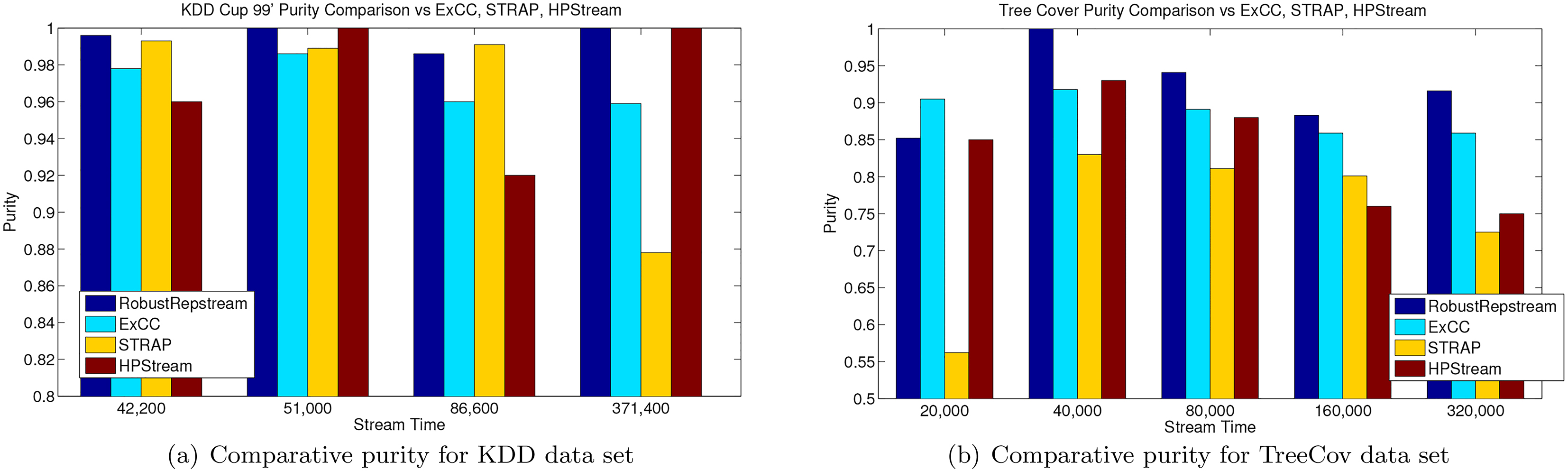
To evaluate the comparative performance of our method we compare against the published results of other stream clustering algorithms. Namely, we compare against the base RepStream algorithm, as well as published results for ExCC [6], STRAP [39], HPStream [2], stream specific algorithms that have shown high quality performance in stream clustering context. The published results favour the purity evaluation metric, which is commonly used for external validation when ground truth class labels are available, as is the case with the KDD Cup and Tree Cover data sets. For our experiments we use a purity horizon of 200 data points, which is a common horizon for the evaluation of clustering algorithms when using purity [3, 2].

Figure 16a shows the comparative purity of the different methods on the KDD data set. RobustRepStream can be seen to perform favourably to the other clustering algorithms in all cases. HPStream results in equal purity at the 51 000 and 371 400 time slices, while STRAP outperforms RobustRepStream slightly during the 86 600 time slice. However, overall our method consistently produces high purity output during the KDD dataset, as we show in further evaluations.

Figure 16b shows the comparative purity for the Tree Cover data set. It is notable that RobustRepStream outperforms the other algorithms using the published results for these methods for all time steps save for the 20 000 time step. ExCC performs consistently highly on this dataset similar to RobustRepStream and has a lower variance in purity over time. However our method does overall outperform it on these published time steps. We show in subsequent evaluations that our method is able to maintain similar high levels of clustering output.

Figure 16.

Comparative results for the KDD and Treecov datasets.

We also compare against the results of the D-Stream [11] and DBStream [18] algorithms, grid-based and micro-cluster density-based stream clustering algorithms respectively, which perform well against the well known CluStream and DenStream algorithms. D-Stream divides the data space into fixed-width cells, and tracks which cells become dense according to input parameters, which allows D-Stream to effectively find arbitrarily shaped parameters. DBStream, on the other hand, is a sophisticated micro-cluster based approach which seeks to solve weaknesses of previous micro-cluster approaches. DBStream allows micro-clusters to overlap, and records the shared density in these overlapping regions. This additional information allows better clustering decisions to be made, as the shared regions give insight into the arrangement of the underlying data points. Both D-Stream and DBStream are high quality stream clustering approaches that perform well against contemporary algorithms. The stream package for R was used to run these algorithms on the data sets. The data sets were normalised between values of 0 and 1 in each data dimension. For each data set the algorithms were parametrised according to the suggested parameter values in the respective papers and the documentation for their implementations. Specifically, D-Stream grid-size parameter was set to $\textit{len}=0.05$ , its dense and sparse cell thresholds set to $C_{m}=3.0$ and $C_{m}=0.8$ , the decay value $\lambda=0.998$ , and its sporadic cell deletion parameter $\beta=0.3$ . The DBStream algorithm was set with its micro-cluster radius $r=0.05$ , its decay parameter $\lambda=0.01$ , its cleanup interval $t\_\textit{gap}=1000$ , the minimum weight $w\_\textit{min}=3.0$ , and its intersection factor $\alpha=0.1$ . The purity horizon, as we noted earlier, is 200, and all the datasets have had all their attributes normalised between 0 and 1.

Figure 17.

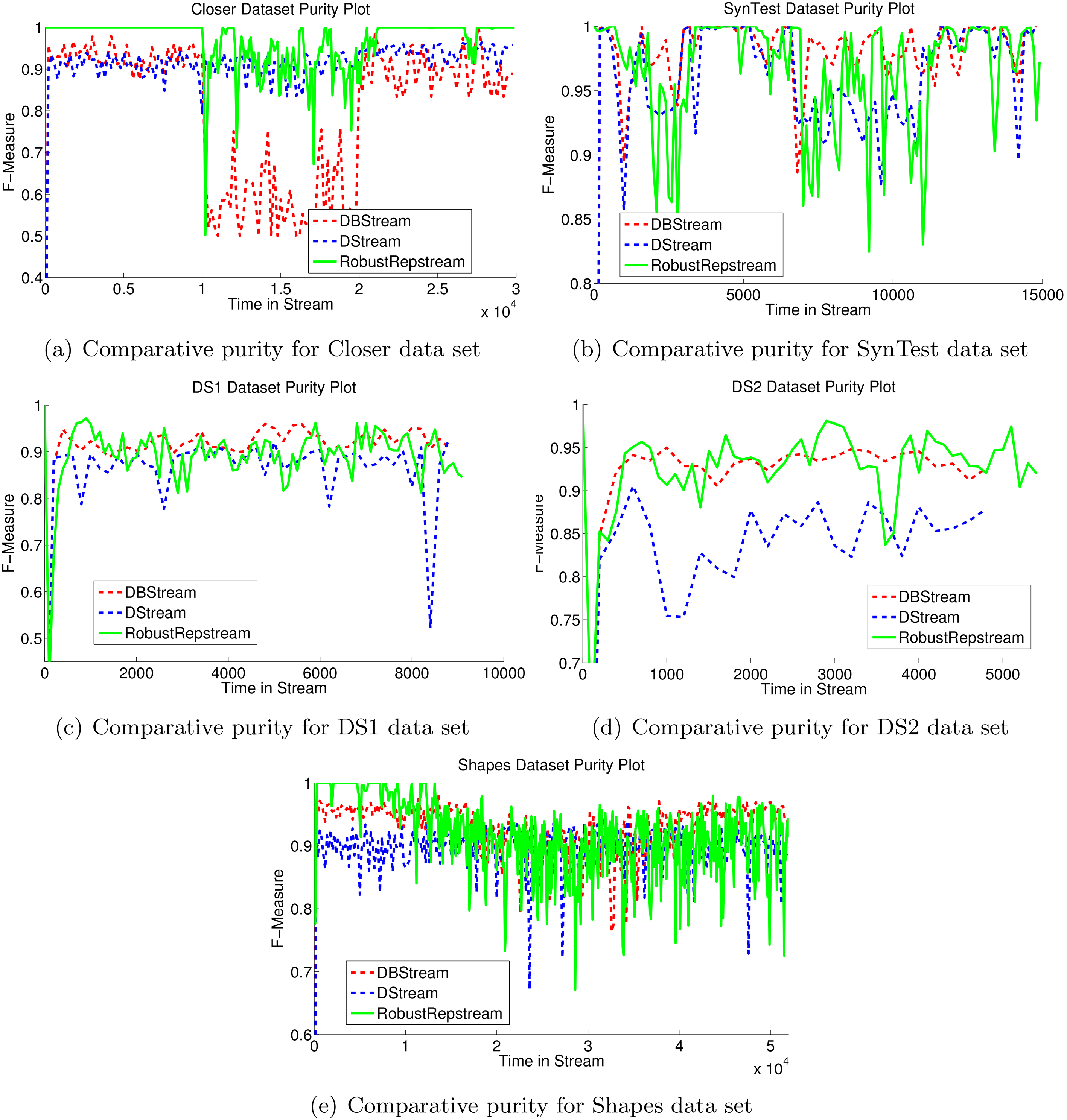
Comparative purity results for synthetic datasets.

Figure 17a shows the comparative purity results for the Closer data set using D-Stream, DBStream, and RobustRepStream. On this data set RobustRepStream outperforms the other algorithms in general over the first and last 10,000 data points, reaching almost 100% purity during these times. during the middle third of the stream, however, DBStream on average has a more consistent higher purity value, possibly due to its shared density feature preventing the overlapping distributions from merging together. RobustRepStream, on the other hand during this period, has periods when its purity value is higher, but also has periods where it achieves a lower purity value than DBStream. As shown in Table 2 however, the overall average purity of RepStream is higher than that of DBStream.

Table 2

Average purity score of DBStream, D-Stream, and RobustRepStream

Data set	DBStream	D-Stream	RobustRepStream
DS1	0.902	0.851	0.893
DS2	0.893	0.812	0.926
SynTest	0.969	0.951	0.966
Closer	0.799	0.913	0.968
Shapes	0.926	0.894	0.918
TreeCov	0.508	0.690	0.884
KDD99	0.993	0.989	0.999

Figure 17b shows the clustering purity for the SynTest data set for the three noted algorithms. On average the three algorithms achieve very similar clustering quality. Table 2 shows how the average (mean) purity differs by only 1.8% between the algorithms, achieving 0.969, 0.951, and 0.966 purity for DBstream, D-Stream, and RobustRepStream respectively.

Figure 17c and d show the clustering results for the DS1 and DS2 data sets respectively. These data sets do not evolve over time or simulate a stream, rather they are static distributions with concave classes, and classes within other classes, making them difficult to cluster. On these data sets the algorithms achieve similar clustering purity. Overall their purity, shown in Table 2, differs very little, though with the graph-based D-Stream performing noticeably worse than the other algorithms. RobustRepStream and DBStream differ in purity by less than 0.03 on average.

Figure 17e shows the purity results achieved for the Shapes data set, which simulated the evolution of a stream, by morphing the size of distributions over time as well as combining two distributions together. For this data set DBstream outperforms both D-Stream and RobustRepStream, achieving average purity 2% higher than D-Stream and 0.8% higher than RobustRepStream.

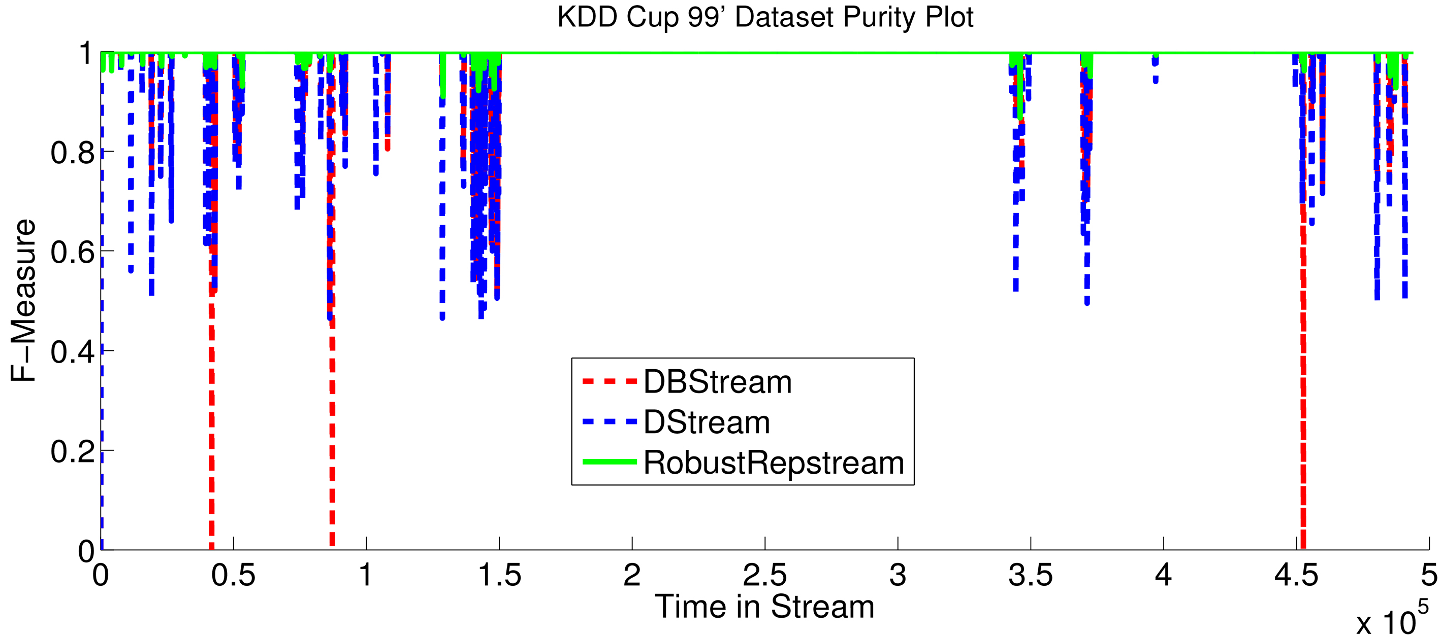
As for the real world benchmark test data sets Fig. 18 shows the purity of the KDD Cup 99’ Network Intrusion data set. For most of the stream all three algorithms achieve perfect purity, due to the presence of only one class for most of the stream. This only differs during the network attack simulations, in which abnormal traffic is inserted into the stream, represented by data points with different class labels mixing in with the typical traffic. During the attacks all algorithms achieve less than perfect purity, with D-Stream performing the worst, having the greatest drops in purity, the average purity for D-Stream over the data set is 0.989. DBStream fares better during the attacks, with an average purity over the whole stream of 0.993. RobustRepStream performs the best on this data set, achieving 0.999 purity on average, and never dropping below 0.9 purity during the length of the stream.

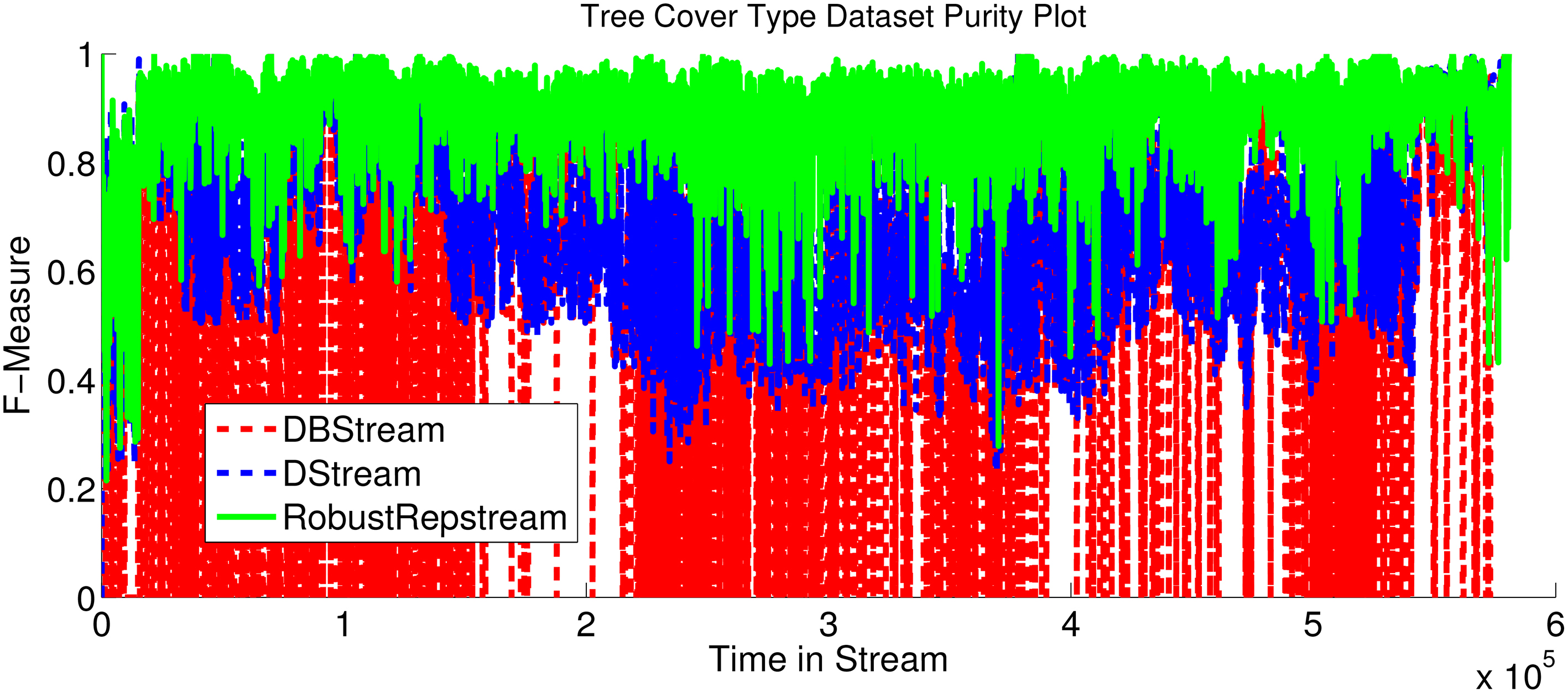
The most stark difference between the clustering algorithms is shown in the Tree Cover Type data set, presented in Fig. 19. This data set is difficult to cluster, having overlapping classes and 10 different attributes for the data. On average RobustRepStream achieves a purity of 0.884, significantly outperforming both D-Stream and DBStream, which achieve 0.690 and 0.508 purity respectively, as shown in Table 2.

Figure 18.

Comparative purity for KDD Cup 99’ data set.

5.5 Baseline for comparison

Because RobustRepStream is an extension of the RepStream algorithm it makes sense to compare its performance to the algorithm on which it is based. RepStream, as shown in its original paper [23] performs well against other stream clustering algorithms. To compare the relative performance of RobustRepStream compared to RepStream we start by determining what our baseline for comparison is. Since we are extending the RepStream method we want to compare against the best possible theoretical performance of RepStream.

To do this we ran multiple instances of RepStream over a range of $K$ values from $K=5$ to $K=30$ , using $\alpha=2.0$ , and using a memory limit of 1000 points and determined which $K$ value produces the best overall performance. The reason for this range is that $K$ values lower than 5 tend to fragment clusters into dozens of tiny clusters, while values higher than 30 tend to put all data points into the same cluster. Additionally the vanilla normalisation method was used, with Manhattan distance as the distance metric.

$F$ measure was calculated every 100 data points, from which we compute the mean $F$ measure over the length of the stream. Table 3 shows the $K$ value which produced the highest overall $F$ measure for each of our test data sets, and the corresponding $F$ measure values. These $K$ values are the ones for which the original RepStream produced the highest overall $F$ measure scores through the length of the stream. We will evaluate our dynamic variation in comparison to these, and will refer to them as the optimal $K$ values.

Table 3
Best $K$ values

Data set	Optimal $K$	Avg $F$ measure
DS1	7	0.7208
DS2	7	0.6371
Closer	9	0.8614
SynTest	9	0.7989
Shapes	6	0.6234
KDD	30	0.7898
TreeCov	29	0.6108

Figure 19.

Comparative purity for Tree Cover data set.

5.6 Evaluation of RobustRepStream

Figure 20.

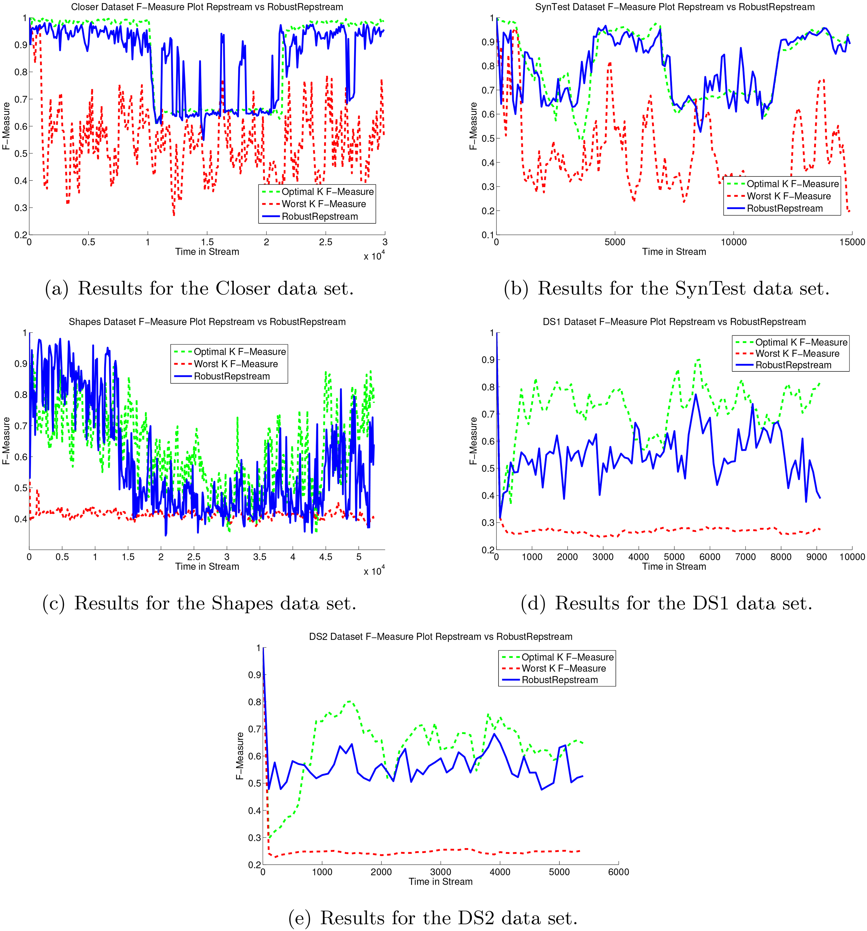
F-Measure results for the synthetic datasets.

Our dynamic version of RepStream was set to run on our evaluation data sets using an $\alpha$ scaling factor value of 2.0, the same as our evaluation baseline. This parameter is also used as the skewness excess threshold, for the reasons mentioned in Section 4.2. The memory limit was set to 1000 points, and used vanilla normalisation, the default value of 0.99 was used for the $\lambda$ decay factor, and Manhattan distance as the distance metric.

Figure 20a shows the $F$ measure of our method on the Closer data set. The dynamic method, plotted in solid blue, follows even closer to the optimal than on the previous data set. The average $F$ measure of 0.7859 of our method compared to 0.8614 (shown in Table 4) for the optimal $k$ leaves an average difference of only 0.0755. Both the worst and mid $K$ values perform better on this data set in comparison, with the worst $K$ value having an average $F$ measure of 0.5435, and the mid $K$ value producing a $F$ measure of 0.8589. This implies that on this data set there is a larger range of $K$ values which produce good clustering results.

Table 4

Average $F$ measure values of base RepStream with the Best, Worst, and in-between $K$ values, compared to our RobustRepStream method

Data set	RobustRepStream	Best $K$	Worst $K$	Avg $K$
Closer	0.8450	0.8614	0.5435	0.8589
SynTest	0.7945	0.7989	0.4345	0.7435
KDD	0.7644	0.7898	0.2636	0.7160
TreeCov	0.5959	0.6108	0.2978	0.6088
Shapes	0.5810	0.6234	0.4140	0.4427
DS1	0.5532	0.7208	0.2767	0.3134
DS2	0.5679	0.6371	0.2594	0.2656

Figure 21.

Results for the KDD data set.

Figure 22.

Results for the Tree Cover data set.

Figure 23.

Sensitivity analysis of the $\alpha$ parameter.

Figure 20b shows the $F$ measure scores of our method and our comparison baselines on the SynTest data set. Our method results in a lower $F$ measure than the best $K$ value over the first and last 10,000 points of the data set, however on average performs better during the middle 10,000 point section. The performance of our method is comparable to that of the mid $K$ value, being only 0.015 different on average, as shown in Table 4. Even so, our method performs, on average, only 0.0569 lower in terms of $F$ measure compared to the best possible single static $K$ value.

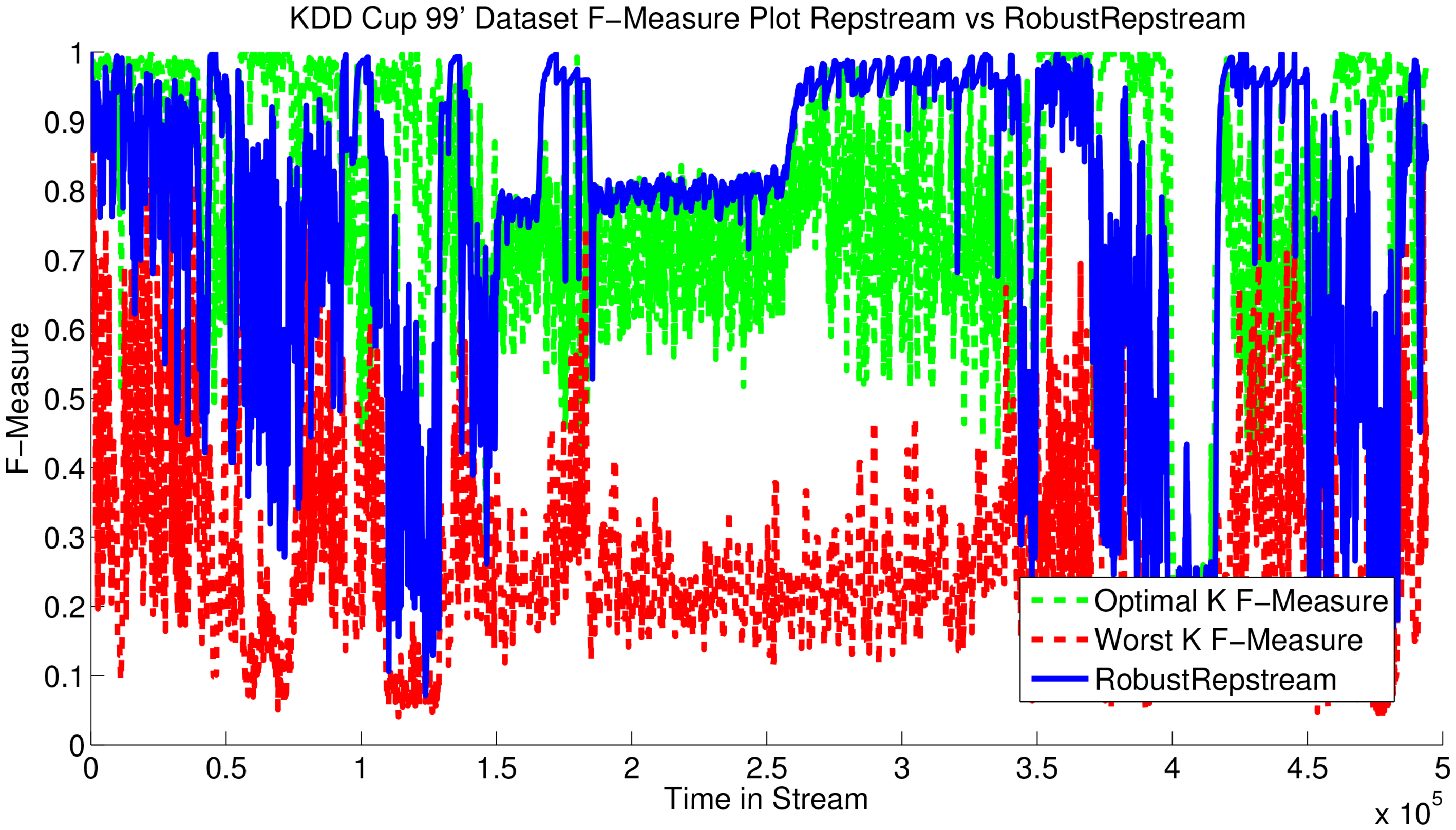
Figure 21 shows the $F$ measure of the RobustRepStream method versus the $F$ measure of the best, worst, and mid single static $K$ values on the KDD Cup 99’ data set. This is a real-world high dimensional benchmark data set often used in clustering algorithm evaluation, which is significantly different from the previous synthetic data sets. Our dynamic method on average produces an $F$ measure value of 0.7035. The optimal $k$ value produced a $F$ measure score of 0.7898 meaning that our method remains on average within 0.1 of the optimal. There are times when our method performs worse, however on average its performance is comparable to the optimal value, when poorly selected input parameters could result in $F$ measure values as low as 0.2636 on average, as shown in Table 4.

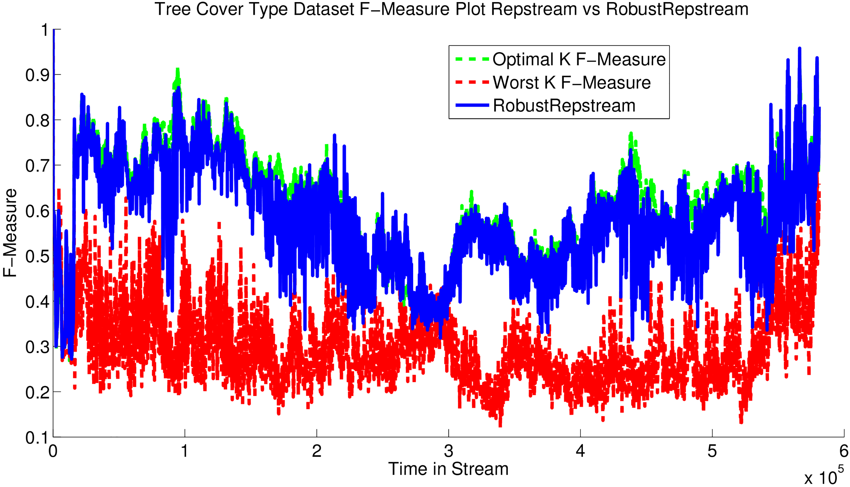
Figure 22 shows the performance of our method on the Tree Cover Type data set. This data set is significantly more difficult to separate classes, with even the optimal $K$ value having an average $F$ measure score of only 0.6108. Whilst the RobustRepStream method performs comparatively worse on this data set compared to the others, it is still on average only 0.1120 below the optimal, as shown in Table 4.

We note that RobustRepStream can still perform almost equivalent to RepStream even when RepStream is supplied with an optimal $K$ value at the beginning of its runtime. However, if optimal parameters cannot be guaranteed, as is to be assumed when dealing with unlabelled data in an unsupervised context, that RobustRepStream outperforms RepStream set with non-optimal parameters.

5.7 Sensitivity

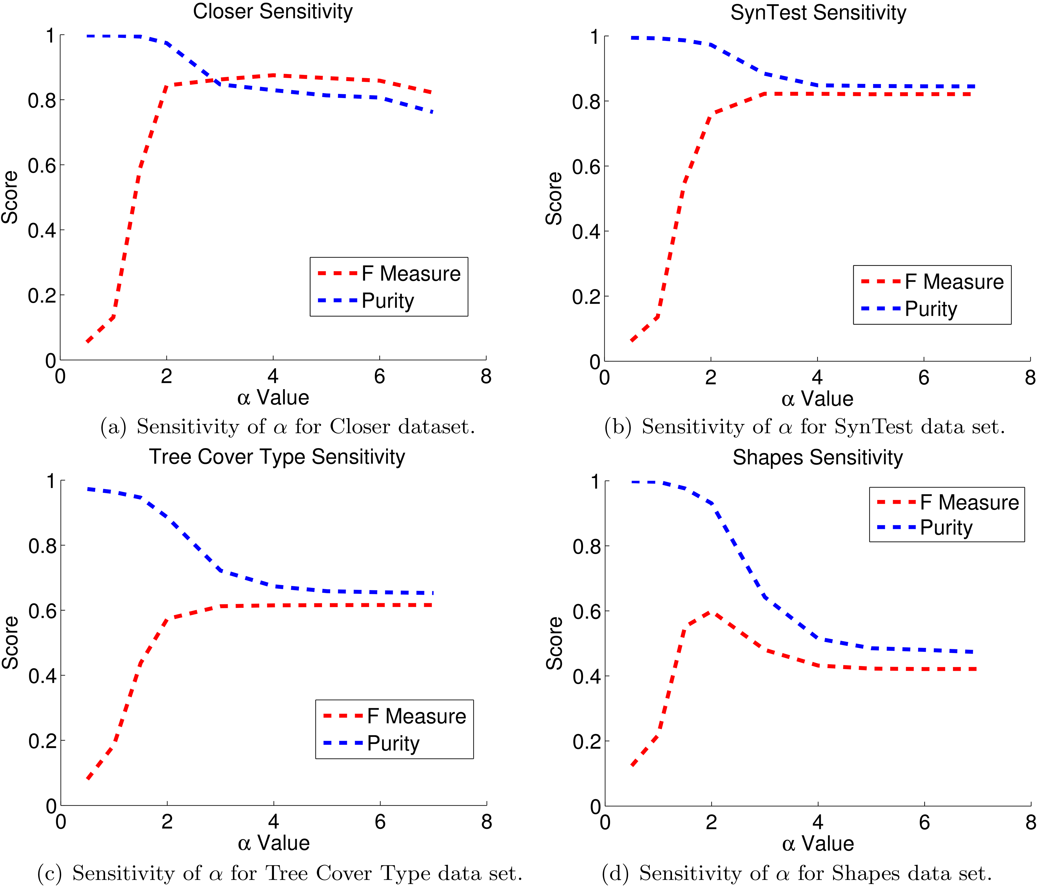
We investigate the sensitivity of the $\alpha$ parameter with regards to clustering quality. Since we remove the $K$ value used by the original RepStream, and replace it with our edge selection process described in Section 4.2, we wish to show how sensitive our changes are. Figure 23a–d show both the purity and $F$ measure scores of some of our datasets.

In all cases $\alpha$ values below 2 produce very low $F$ measure values whilst producing very high purity values. This is due to under-clustering, where the algorithm is resulting in too many clusters containing too few points. We expect this result as we described earlier.

At higher values, around $2\leqslant\alpha\leqslant 3$ , the $F$ measure increases and plateaus thereafter, whilst the purity value decreases to a roughly stable level. From these sensitivity tests we show that an $\alpha$ value of between 2 and 3 consistently results in the best balance between purity and $F$ measure scores. We note that increases in $F$ measure, which measures both precision and recall, can be achieved with higher $\alpha$ values, however the improvements in the cases of our sensitivity experiments, are marginal.

6. Results discussion

In Section 5 we compare RobustRepStream against the published results of several other stream clustering algorithms, specifically STRAP, ExCC, HPStream, and the more recent D-Stream and DBstream.

As shown in the comparative purity results in Fig. 16a and b, RobustRepStream performs well against the results published for RepStream, ExCC, STRAP, and HPStream. RobustRepStream results in similar clustering quality to RepStream in almost all cases, and outperforms RepStream slightly in purity on the Tree Cover Type data set.

Compared to the algorithms D-Stream and DBstream, RobustRepStream performs very favourably. DBstream marginally outperforms RobustRepStream on the SynTest, DS1, DS2, and Shapes data set very marginally, as shown in Table 2, however RobustRepStream performs very favourably compared to these algorithms on the Closer, Tree Cover, and KDD99’ data sets. It is worth noting that these results are achieved with all algorithms using the same input parameters for all data sets. Without tuning the parameters RobustRepStream performs comparably to the other algorithms, and outperforms them on the real-world benchmark data sets.

Compared to RepStream, the RobustRepStream algorithm performs well. Even when comparing to the best case, setting RepStream optimally, the RobustRepStream algorithm with no parameter adjustment between data sets has similar performance in terms of $F$ measure to RepStream using the best possible value for the $K$ parameter. This is notable in the 2-dimensional synthetic datasets, as well as the benchmark datasets – Tree Cover and KDD Cup, which have 10 and 43 dimensions respectively, which demonstrates that our method is able to perform on datasets with varying levels of dimensionality.

RobustRepStream is an extension of the RepStream algorithm with the goal of reducing the need for users to set the input parameters, these experiments show that by using the same parameter values for all data sets the RobustRepStream algorithm is able to perform similarly to RepStream even though the RepStream algorithm has the advantage of being tuned for the data set. This situation is unrealistic in the favour of RepStream because one can’t expect to know what the best parameter values are before beginning, so this comparison is made to a hypothetical best case, yet still performs well.

In terms of sensitivity the value chosen for the $\alpha$ threshold seems to be insensitive to the data set used. In Section 5.7 we show the purity values of RobustRepStream run at different $\alpha$ values on various data sets. In our experiments we used $\alpha=2$ to represent that each vertex may have one or fewer anomalous outgoing edges, and this value achieves very high quality results in terms of purity. The highest combination of purity and $F$ measure score is achieved with a value between $2\leqslant\alpha\leqslant 3$ in the tested data sets. Whereas the $K$ value of RepStream needed to be adjusted for each data set in order to achieve the highest quality performance, our method provides consistently high quality clustering output without the need to tune our hyper parameters for all the data sets that we tried. This is in line with our goal of removing the need for users to set the sensitive $K$ parameter in RepStream and of making the algorithm more robust.

7. Conclusion

In this paper we introduced a clustering algorithm, RobustRepStream, an extension of the RepStream algorithm, that removes the need to set its primary input parameter, the $K$ value, which directly affects the interconnectivity of its graph-based structure. We employ a computed feature called the skewness excess to automatically set the number of outgoing edges for each vertex in the graph automatically and dynamically over time. Our method selects the local connectivity parameter as the maximum value at which the skewness excess is still below a pre-defined universal threshold. This process is performed continuously on new vertices into the graph, and for any nearby vertices for which the new vertex becomes a potential neighbour. Using this method we maintain a non-static and non-uniform number of outgoing edges for vertices in the graph.

We propose that this same approach can be applied in any situation in which a $K$ -NN graph would be used. The ability to dynamically set the number of outgoing edges on a per-vertex basis reduces the dependence on knowing an appropriate $K$ value. We further propose that the usage of the skewness excess in determining outgoing edges in a directed nearest neighbour graph can be generalised and used in building graphs in situations where a static $K$ value is not appropriate. This method of selecting edges is not unique to the RobustRepStream algorithm, and could be applied in any nearest neighbour graph-based context. We expect future findings will confirm our conjecture.

Our method successfully removes the need for the user to set the $K$ parameter which is crucial for the success of the original RepStream algorithm. By making use of the $\alpha$ value which is already set by the user as a threshold our RobustRepStream algorithm can achieve performance comparable to that of RepStream when it has an optimally set $K$ value. Given that it is virtually impossible to know what the optimal $K$ value would be for an unlabelled data set, this results in one fewer sensitive parameter which needs to be set for the algorithm. RepStream is shown to be much less sensitive in terms of performance variance for the remaining parameter, the $\alpha$ scaling factor than to the $K$ value. As we show in Section 5.7, this parameter is far less sensitive, and results in consistent clustering quality across different datasets in RobustRepStream. This is in contrast to the sensitive nature of the $K$ parameter, which as we show in Table 3 requires very different values from data set to data set.

We have shown experimentally on average for the data sets that evolve over time that our RobustRepStream performs within an $F$ measure margin of 0.03 of the best possible performance that could be achieved by RepStream when the ground-truth is known. For all of our evaluation data sets, setting the $K$ value non-optimally can lead to $F$ measure differences of more than 0.3 compared to the optimal values. This demonstrates the importance that the $K$ parameter had on RepStream and why removing the need to set the $K$ parameter is so valuable.

References

Ackermann

M.R.

Märtens

Raupach

Swierkot

Lammersen

and Sohler

, Streamkm+⁣+: a clustering algorithm for data streams, Journal of Experimental Algorithmics 17 (2012), 2–4.

Aggarwal

Han

Wang

and Yu

, A Framework for Projected Clustering of High Dimensional Data Streams, in: Proceedings 2004 VLDB Conference, Elsevier, 2004, pp. 852–863.

Aggarwal

C.C.

P.S.

Han

and Wang

, A Framework for Clustering Evolving Data Streams, in: Proceedings 2003 VLDB Conference, Elsevier, 2003, pp. 81–92.

Amini

Wah

T.Y.

and Saboohi

, On density-based data streams clustering algorithms: a survey, Journal of Computer Science and Technology 29(1) (Jan 2014), 116–141.

Barddal

J.P.

Gomes

H.M.

and Enembreck

, SNCStream: A Social Network-based Data Stream Clustering Algorithm, in: Proceedings of the 30th Annual ACM Symposium on Applied Computing – SAC ’15, SAC ’15, New York, New York, USA, 2015, pp. 935–940. ACM Press.

Bhatnagar

Kaur

and Chakravarthy

, Clustering data streams using grid-based synopsis, Knowledge and Information Systems 41(1) (Oct 2014), 127–152.

Blackard

J.A.

and Dean

D.J.

, Comparative accuracies of artificial neural networks and discriminant analysis in predicting forest cover types from cartographic variables, Computers and Electronics in Agriculture 24(3) (1999), 131–151.

Cagnini

H.E.L.

and Barros

R.C.

, PASCAL: An EDA for parameterless shape-independent clustering, in: 2016 IEEE Congress on Evolutionary Computation (CEC), IEEE, Jul 2016, pp. 3433–3440.

Callister

Lazarescu

and Pham

D.-S.

, Graph-based clustering with drepstream, in: Proceedings of the Symposium on Applied Computing, SAC ’17, New York, NY, USA, 2017, pp. 850–857. ACM.

10.

Cao

Estert

Qian

and Zhou

, Density-Based Clustering over an Evolving Data Stream with Noise, in: Proceedings of the 2006 SIAM International Conference on Data Mining, Society for Industrial and Applied Mathematics, Philadelphia, PA, Apr 2006, pp. 328–339.

11.

Chen

and Tu

, Density-based clustering for real-time stream data, in: Proceedings of the 13th ACM SIGKDD International Conference on Knowledge Discovery and Data Mining – KDD ’07, New York, New York, USA, 2007, pp. 133. ACM, ACM Press.

12.

Ding

Zhang

Jia

and Qian

, An adaptive density data stream clustering algorithm, Cognitive Computation 8(1) (Feb 2016), 30–38.

13.

Forestiero

Pizzuti

and Spezzano

, A single pass algorithm for clustering evolving data streams based on swarm intelligence, Data Mining and Knowledge Discovery 26(1) (Jan 2013), 1–26.

14.

Foss

and Zaiane

O.R.

, A parameterless method for efficiently discovering clusters of arbitrary shape in large datasets, in: Proc. the 2002 IEEE Int Conf on Data Mining, ICDM 2003, 2002, pp. 179–186.

15.

Gao

Zhang

and Tan

P.-N.

, An Incremental Data Stream Clustering Algorithm Based on Dense Units Detection, in: Ho

T.B.

Cheung

and Liu

, eds, Proceedings of the 9th Pacific-Asia Conference on Advances in Knowledge Discovery and Data Mining, Hanoi, Vietnam, 2005, pp. 420–425. Springer.

16.

Gouineau

Landry

and Triplet

, PatchWork, a scalable density-grid clustering algorithm, in: Proceedings of the 31st Annual ACM Symposium on Applied Computing – SAC ’16, SAC ’16, New York, New York, USA, 2016, pp. 824–831. ACM Press.

17.

Guha

Mishra

Motwani

and O’Callaghan

, Clustering data streams, in: Proceedings of the Annual Symposium on Foundations of Computer Science, 2000, pp. 359–366.

18.

Hahsler

and Bolaos

, Clustering data streams based on shared density between micro-clusters, IEEE Transactions on Knowledge and Data Engineering 28(6) (Jun 2016), 1449–1461.

19.

Hassani

Spaus

and Seidl

, Adaptive Multiple-Resolution Stream Clustering, in: 2016 16th IEEE/ACM International Symposium on Cluster, Cloud and Grid Computing (CCGrid), IEEE, May 2014, pp. 134–148.

20.

Hettich

and Bay

S.D.

, The UCI KDD Archive [http://kdd.ics.uci.edu], 1999.

21.

Kaur

Bhatnagar

and Chakravarthy

, Stream Clustering Algorithms: A Primer, in: Big Data in Complex Systems, Springer, Vol. 9, 2015, pp. 105–145.

22.

Lee

G.H.

, Grid-based dynamic clustering with grid proximity measure, Intelligent Data Analysis 20(4) (2016), 853–875.

23.

Lühr

and Lazarescu

, Incremental clustering of dynamic data streams using connectivity based representative points, Data & Knowledge Engineering 68(1) (Jan 2009), 1–27.

24.

Maier

Hein

and Von Luxburg

, Cluster identification in nearest-neighbor graphs, in: Proc. the 18th Int Conf on Algorithmic Learning Theory, Springer, 2007, pp. 196–210.

25.

Mansalis

Ntoutsi

Pelekis

and Theodoridis

, An evaluation of data stream clustering algorithms, Statistical Analysis and Data Mining: The ASA Data Science Journal 11(4) (2018), 167–187.

26.

Mohd

W.M.B.W.

Beg

Herawan

and Rabbi

, An improved parameter less data clustering technique based on maximum distance of data and lioyd k-means algorithm, Procedia Technology 1 (2012), 367–371.

27.

Nguyen

H.-L.

Woon

Y.-K.

and Ng

W.-K.

, A survey on data stream clustering and classification, Knowledge and Information Systems 45(3) (2015), 535–569.

28.

O’callaghan

Meyerson

Motwani

Mishra

and Guha

, Streaming-data algorithms for high-quality clustering, in: Proc. the 18th Int Conf on Data Engineering, IEEE, 2002, pp. 0685.

29.

Rousseeuw

P.J.

and Croux

, Alternatives to the median absolute deviation Journal of the American Statistical Association 88(424) (1993), 1273–1283.

30.

Schneider

and Vlachos

, Fast parameterless density-based clustering via random projections, in: Proceedings of the 22nd ACM International Conference on Conference on Information & Knowledge Management – CIKM ’13, New York, New York, USA, 2013, pp. 861–866. ACM, ACM Press.

31.

Silva

J.A.

Faria

E.R.

Barros

R.C.

Hruschka

E.R.

de Carvalho

A.C.

and Gama

, Data stream clustering: a survey, ACM Computing Surveys (CSUR) 46(1) (July 2013), 13.

32.

Sun

Guo

Liu

and Xiong

, Fast affinity propagation clustering based on incomplete similarity matrix, Knowledge and Information Systems 51(3) (Jun 2017), 941–963.

33.

Sun

Guo

Liu

and Xiong

, Fast affinity propagation clustering based on incomplete similarity matrix, Knowledge and Information Systems 51(3) (2017), 941–963.

34.

Tseng

V.S.

and Kao

C.-P.

, Efficiently mining gene expression data via a novel parameterless clustering method, IEEE/ACM Transactions on Computational Biology and Bioinformatics 2(4) (Oct 2005), 355–365.

35.

Wan

W.K.

Dang

X.H.

P.S.

and Zhang

, Density-based clustering of data streams at multiple resolutions, ACM Transactions on Knowledge Discovery from Data 3(3) (Jul 2009), 1–28.

36.

Wattanakitrungroj

Maneeroj

and Lursinsap

, Bestream: Batch capturing with elliptic function for one-pass data stream clustering, Data & Knowledge Engineering (2018).

37.

Widmer

and Kubat

, Learning in the presence of concept drift and hidden contexts, Machine Learning 23(1) (1996), 69–101.

38.

Cao

Tian

and Alabdulkarim

, A comparative study of clustering ensemble algorithms, Computers & Electrical Engineering 68 (2018), 603–615.

39.

Zhang

Furtlehner

and Sebag

, Data streaming with affinity propagation, in: Proc. Joint European Conference on Machine Learning and Knowledge Discovery in Databases, Springer, 2008, pp. 628–643.

40.

Zhou

Cao

Qian

and Jin

, Tracking clusters in evolving data streams over sliding windows, Knowledge and Information Systems 15(2) (May 2008), 181–214.

41.

Zhu

and Jiang

, A consistency-based validation for data clustering, Intelligent Data Analysis 19(3) (2015), 471–484.

RobustRepStream: Robust stream clustering using self-controlled connectivity graph

Abstract

Keywords

1. Introduction

2.1 Stream clustering algorithms

2.1.1 Micro-cluster clustering

2.1.2 Graph clustering

2.1.3 Grid based clustering

2.1.4 Other approaches

Table 1 Table showing the input parameters used for each algorithm.

3. Preliminaries

3.1 RepStream graph structures

3.1.1 The point-level graph

3.1.2 The representative-level graph

3.2 Clustering with density relation

• The computation of the skewness excess score of the distribution of normalised edge lengths at each vertex. • Automatic model selection based on the computed skewness excess score. 4.1 Skewness excess

.

.

5.1 Real world data sets: KDD and Tree Cover

5.1.1 The KDD Cup 1999 data set

5.1.2 The Tree Cover Type data set

5.2 Synthetic data sets

5.2.1 Closer data set

5.4 Comparison to other algorithms

Table 3 Best K values

6. Results discussion

7. Conclusion

References

Table 1
Table showing the input parameters used for each algorithm.

•
The computation of the skewness excess score of the distribution of normalised edge lengths at each vertex.
•
Automatic model selection based on the computed skewness excess score.

4.1 Skewness excess

Table 3
Best $K$ values