Fourier neural networks: A comparative study

Abstract

We review neural network architectures which were motivated by Fourier series and integrals and which are referred to as Fourier neural networks. These networks are empirically evaluated in synthetic and real-world tasks. Neither of them outperforms the standard neural network with sigmoid activation function in the real-world tasks. All neural networks, both Fourier and the standard one, empirically demonstrate lower approximation error than the truncated Fourier series when it comes to approximation of a known function of multiple variables.

Keywords

Neural networks Fourier series function approximation convergence

1. Introduction

Machine learning is an actively developing area studying algorithms and statistical models that perform specific tasks without using explicit instructions, relying on patterns and inference instead. It is seen as a subset of artificial intelligence. Machine learning algorithms build a mathematical model based on sample data, known as “training data”, in order to make predictions or decisions without being explicitly programmed to perform the task [26, 6]. For example, in image recognition, they might learn to identify images that contain cats by analyzing example images that have been manually labeled as “cat” or “no cat” and using the results to identify cats in other images. They do this without any prior knowledge of cats, for example, that they have fur, tails, whiskers and cat-like faces. Instead, they automatically generate identifying characteristics from the examples that they process. Machine learning algorithms are used in a wide variety of applications, such as email filtering and computer vision, where it is difficult or infeasible to develop a conventional algorithm for effectively performing the task.

Artificial neural networks (ANN) are machine learning models vaguely inspired by the biological neural networks that constitute animal brains. An ANN is based on a collection of connected units or nodes called artificial neurons, which loosely model the neurons in a biological brain (Fig. 1).

Figure 1.

An artificial neural network as an interconnected group of nodes (left). Neuron and myelinated axon, with signal flow from inputs at dendrites to outputs at axon terminals (right). Source: Wikipedia.

Each connection, like the synapses in a biological brain, can transmit a signal to other neurons. An artificial neuron that receives a signal then processes it and can signal neurons connected to it. In ANN implementations, the “signal” at a connection is a real number, and the output of each neuron is computed by some non-linear function of the sum of its inputs. The connections are called edges. Neurons and edges typically have a weight that adjusts as learning proceeds. The weight increases or decreases the strength of the signal at a connection. Neurons may have a threshold such that a signal is sent only if the aggregate signal crosses that threshold. Typically, neurons are aggregated into layers. Different layers may perform different transformations on their inputs. Signals travel from the first layer (the input layer), to the last layer (the output layer), possibly after traversing the layers multiple times.

The original goal of the ANN approach was to solve problems in the same way that a human brain would. However, over time, attention moved to performing specific tasks, leading to deviations from biology. ANNs have been used on a variety of tasks, including computer vision, speech recognition, machine translation, social network filtering, playing board and video games, medical diagnosis and even in activities that have traditionally been considered as reserved to humans, like painting [11].

In this work we explore several neural network architectures, the authors of which were inspired by Fourier analysis, the branch of mathematics that studies the way general functions may be represented or approximated by sums of simpler trigonometric functions. Fourier analysis grew from the study of Fourier series, and is named after Joseph Fourier, who showed that representing a function as a sum of trigonometric functions greatly simplifies the study of heat transfer. We will collectively refer to the NN architectures inspired by the Fourier analysis as Fourier Neural Networks (FNNs). First FNNs were proposed in 80s and 90s, but they are not widely used nowadays. Is there any reasonable explanation for this, or were they simply not given enough attention? To answer this question we perform empirical evaluation of the FNNs, found in the existing literature, on synthetic and real-world datasets. We are mainly interested in the following hypotheses: Is any of the FNNs superior to others? Does any FNN outperform conventional feedforward neural network with the logistic sigmoid activation? Our experiments show that the FNN of [10] outperforms all other FNNs, and that all FNNs are not better than the standard feedforward neural architecture with sigmoid activation function except the case of modeling synthetic data.

2. Related work

Approximation properties of standard feedforward neural networks were studied earlier by Hornik et al. [14], Cybenko [7]. The approximation error bound for such networks was first derived by Barron[4]. The study of convergence rates of Fourier series goes back to 1960-s and we refer the reader to the works of Alimov et al. [2, 3] for a survey of the results in this area.

The first Fourier Neural Networks were introduced by Gallant and White[10], who also showed that their networks possess the convergence guarantees of the Fourier series. McCaffrey and Gallant [22] derived the approximation error bound for the FNN of Gallant and White[10]. Later, Silvescu[27] introduced another type of a FNN, but did not investigate its approximation error. Finally, Liu [20] suggested one more version of a FNN, but did only empirical evaluation of its performance.

To the best of our knowledge, our work is the first one that compares systematically the known Fourier Neural Networks on synthetic and real-world data.

3. Preliminaries

Notation. We let $\mathbb{Z}$ and $\mathbb{R}$ denote the integer and real numbers, respectively. Bold-faced letters ( $\mathbf{x}$ , $\mathbf{y}$ ) denote vectors in $d$ -dimensional Euclidean space $\mathbb{R}^{d}$ , and plain-faced letters ( $x$ , $f$ ) denote either scalars or functions. $\langle\cdot,\cdot\rangle$ denotes inner product: $\langle\mathbf{x},\mathbf{y}\rangle:=\sum_{j=1}^{d}x_{j}y_{j}$ ; and $\|\cdot\|$ , $\|\cdot\|_{2}$ denote the Euclidean norm: $\|\mathbf{x}\|:=\|\mathbf{x}\|_{2}:=\sqrt{\langle\mathbf{x},\mathbf{x}\rangle}$ .

Feedforward neural networks. Following a standard convention, we define a feedforward neural network with one hidden layer of size $n$ on inputs in $\mathbb{R}^{d}$ as

$\displaystyle\mathbf{x}\mapsto v_{0}+\sum_{k=1}^{n}v_{k}\sigma(\langle\mathbf{% x},\mathbf{w}_{k}\rangle+b_{k})$ (1)

where $\sigma(\cdot)$ is the activation function, and $v_{k},b_{k}\in\mathbb{R}$ , $\mathbf{w}_{k}\in\mathbb{R}^{d}$ , $k=1,\ldots,n$ , are parameters of the network. The universal approximation theorem [14, 7] states that a feedforward network Eq. (1) with any “squashing” activation function $\sigma(\cdot)$ , such as the logistic sigmoid function, can approximate any Borel measurable function $f(\mathbf{x})$ with any desired non-zero amount of error, provided that the network is given enough hidden layer size $n$ . Universal approximation theorems have also been proved for a wider class of activation functions, which includes the now commonly used ReLU[19]. The neural network (1) with logistic sigmoid activation $\sigma(x):=1/(1+e^{-x})$ is referred to as standard or vanilla feedforward neural network.

Fourier series. Let $f(\mathbf{x})$ be a function integrable in the $d$ -dimensional cube $[-\pi,\pi]^{d}$ . The Fourier series of the function $f(\mathbf{x})$ is the series

$\displaystyle\sum_{\mathbf{k}\in\mathbb{Z}^{d}}\hat{f}_{\mathbf{k}}e^{i\langle% \mathbf{x},\mathbf{k}\rangle},$ (2)

where the numbers $\hat{f}_{\mathbf{k}}$ , called Fourier coefficients, are defined by

$\displaystyle\hat{f}_{\mathbf{k}}:=(2\pi)^{-d}\underset{[-\pi,\pi]^{d}}{\int}f% (\mathbf{y})e^{-i\langle\mathbf{y},\mathbf{k}\rangle}d\mathbf{y},$

Conceptually, the feedforward neural network with one hidden layer Eq. (1) and the partial sum of the Fourier series Eq. (2) are similar in a sense that both are linear combinations of non-linear transformations of the input $\mathbf{x}$ . The major differences between them are as follows:

•

The Fourier series has a direct access to the function $f(\mathbf{x})$ being approximated, whereas the neural network does not have it – instead it is usually given a training set of pairs $\{\mathbf{x}_{i},f(\mathbf{x}_{i})+\epsilon_{i}\}$ , where $\epsilon_{i}$ is a noise (error).

•

The coefficients and linear transformations of the input in the Fourier series are fixed, but they are trainable in the neural network and are subject to estimation based on the training set $\{\mathbf{x}_{i},f(\mathbf{x}_{i})+\epsilon_{i}\}$ .

There exists a variety of results on convergence of different types of partial sums (rectangular, square, spherical) of the multiple Fourier series Eq. (2) to $f(\mathbf{x})$ in various senses (uniform, mean, almost everywhere). We refer the reader to the works of [2, 3] for a survey of such results. It seems that the existence of such convergence guarantees has motivated several authors to design the activation functions for Eq. (1) in such a way that the resulting neural networks mimic the behavior of the Fourier series Eq. (2). In the next section we give a brief overview of such networks.

4. Overview of the Fourier neural networks

FNN of Gallant and White[10]: The earliest attempt on making a neural network resemble the Fourier series is due to Gallant and White[10] who have suggested the “cosine squasher”

$\displaystyle\sigma_{\text{GW}}(x):=\begin{cases}0,&x\in(-\infty,-\frac{\pi}{2% }),\\ \frac{1}{2}\left(\cos\left(x+\frac{3\pi}{2}\right)+1\right),&x\in[-\frac{\pi}{% 2},\frac{\pi}{2}],\\ 1,&x\in(\frac{\pi}{2},+\infty),\end{cases}$ (3)

as an activation function in the feedforward network Eq/ (1). Moreover, they show that when additionally the connections $\mathbf{w}_{i}$ , $b_{i}$ from input to hidden layer are hardwired in a special way, the obtained feedforward network yields a Fourier series approximation to a given function $f(\mathbf{x})$ . Thus, such networks possess all the approximation properties of Fourier series representations. In particular, approximation to any desired accuracy of any square integrable function can be achieved by such a network, using sufficiently many hidden units. McCaffrey and Gallant[22] showed that the squared approximation error for sufficiently smooth functions is of order $O(n^{-1})$ , where $n$ is the network’s hidden layer size. We notice here that Barron[4] has established the same order of the approximation error for the feedforward networks with any sigmoidal activation1

A bounded measurable function $\phi(x)$ on the real line is called sigmoidal if $\phi(x)\to 1$ as $x\to+\infty$ and $\phi(x)\to 0$ as $x\to-\infty$ .

and when the function being approximated

f(\mathbf{x})

has a bound on the first moment of the magnitude distribution of the Fourier transform. FNN of Gallant and White[10] is denoted as

f_{\text{GW}}

FNN of Silvescu[27]: Another attempt to mimic the behavior of the Fourier series by a neural network was done by Silvescu[27], who introduced the following FNN:

$\displaystyle f_{\text{S}}:\mathbf{x}\mapsto v_{0}+\sum_{k=1}^{n}v_{k}\sigma_{% \text{S}}(\mathbf{x};\bm{\omega}_{k},\bm{\phi}_{k}),$ (4)

with

$\displaystyle\sigma_{\text{S}}(\mathbf{x};\bm{\omega}_{k},\bm{\phi}_{k}):=% \prod_{j=1}^{d}\cos(\omega_{kj}x_{j}+\phi_{kj}),$ (5)

where $\bm{\omega}_{k},\bm{\phi}_{k}\in\mathbb{R}^{d}$ , $v_{k}\in\mathbb{R}$ are trainable parameters. As we can see, Silvescu’s FNN Eq. (4) does not follow the framework of the standard feedforward neural networks Eq. (1), and moreover its activation function is not sigmoidal. Figure 2 depicts the difference between Eqs (1) and (4) for the case when $d=3$ and $n=2$ .

Figure 2.

Standard feedforward NN (top) vs Silvescu’s Fourier NN (bottom). In the standard NN non-linearity is applied on top of the linear transformation of the whole input, whereas in the Silvescu’s network non-linearity is applied separately to each component of the input vector.

Because of this difference, the result of Barron[4] is not applicable to Silvescu’s FNN. However, we conjecture that the same convergence rate is valid for the Silvescu’s FNN. The proof (or disproof) of this conjecture is deferred to our future work.

FNN of Liu[20]: More recently, several authors suggested the following architecture

$\displaystyle f_{\text{L}}:\mathbf{x}\mapsto v_{0}+\sum_{k=1}^{n}v_{k}\cos(% \langle\mathbf{w}_{k},\mathbf{x}\rangle+b_{k})+u_{k}\sin(\langle\mathbf{p}_{k}% ,\mathbf{x}\rangle+q_{k}),$ (6)

where $\mathbf{w}_{k},\mathbf{p}_{k}\in\mathbb{R}^{d}$ , $b_{k},q_{k}\in\mathbb{R}$ are either hardwired or trainable, and $v_{k},u_{k}\in\mathbb{R}$ are trainable parameters. Tan[28] explored aircraft engine fault diagnostics using Eq. (6), Zuo and Cai[29, 30], Zuo et al. [31] used it for the control of a class of uncertain nonlinear systems. The above-mentioned authors did not provide rigorous mathematical analysis of this architecture, instead they used it as an ad-hoc solution in their engineering tasks. Although this FNN fits into the general feedforward framework Eq. (1), its activations are not sigmoidal, and thus the result of Barron[4] is not applicable here as well. Liu [20] empirically evaluated Eq. (6) on various datasets and showed that in certain cases it converges faster than the feedforward network with sigmoid activation and has equally good predicting accuracy and generalization ability. Also, only in the work of Liu [20] all the weights in Eq. (6) are allowed to be trainable, hence we refer to this architecture as $f_{\text{L}}$ .

5. Empirical evaluation

In this section we will perform empirical evaluation of the Fourier neural networks $f_{\text{GW}}$ , $f_{\text{S}}$ , $f_{\text{L}}$ from Section 4 against vanilla feedforward network Eq. (1) with sigmoid activation2

²
I.e. we put $\sigma(x):=\frac{1}{1+\exp(-x)}$ in Eq. (1).

on synthetic and real-world datasets. By “synthetic datasets” we mean datasets generated from a known function. In this case we can also compare the performance of Fourier neural networks to the approximation error given by the partial Fourier series.

5.1 Synthetic tasks

We try to approximate a function of one variable $x\mapsto|x|$ , $x\in[-\pi,\pi]$ , and a function of $d=100$ variables: $\mathbf{x}\mapsto\mathbb{I}[\|\mathbf{x}\|\leqslant 1]$ , $\mathbf{x}\in\{\mathbf{x}\in\mathbb{R}^{100}:\,\|\mathbf{x}\|\leqslant 2\}$ , where $\mathbb{I}[\cdot]$ is the indicator function.3

³
This means that $\mathbb{I}[\|\mathbf{x}\|\leqslant 1]=1$ if $\|\mathbf{x}\|\leqslant 1$ , and 0 otherwise.

In both cases we sampled

5\cdot 10^{5}

data instances uniformly from the domains of the functions. To each instance, we associated a target value according to the target function

|x|

\mathbb{I}[\|\mathbf{x}\|\leqslant 1]

. We did not add noise to the target values. Another

10\cdot 10^{4}

examples were generated in a similar manner, of which

5\cdot 10^{4}

examples were used as a validation set, and

5\cdot 10^{4}

examples were used as a test set. We trained 32 networks on these datasets: for each of the above-mentioned models (vanilla feedforward network,

f_{\text{GW}}

f_{\text{S}}

f_{\text{L}}

) we varied the hidden layer size from 100 to 800 with the step 100. Training was performed with Adam optimizer (Algorithm 5.1) using the TensorFlow ([1]) library.4

⁴

Our implementation of FNNs is available at https://github.com/zh3nis/FNN.

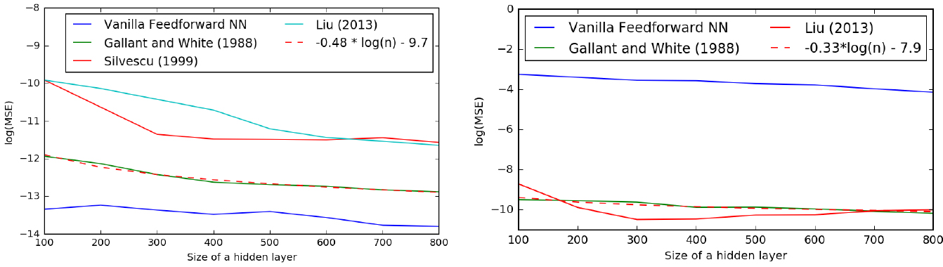
We used the squared loss

l(y,\hat{y}):=(y-\hat{y})^{2}

and batches of size 100. For each model, a learning rate was tuned separately on the validation set. The results are presented in Fig. 3. Vanilla feedforward network Eq. (1) obtains lowest mean squared error (MSE) for

|x|

, whereas the FNN of [10] outperforms all other models for

\mathbb{I}[\|\mathbf{x}\|\leqslant 1]

. According to the regression fits (dashed curves in Fig. 3), the function

x\mapsto|x|

is approximated by the neural networks with error

O(n^{-0.48})

, and this is much worse than the approximation error given by the partial sums of the Fourier series of

f(x)=|x|

, which, according to Lemma 1 below, is of order

O(n^{-3})

. For the function

\mathbf{x}\mapsto\mathbb{I}[\|\mathbf{x}\|\leqslant 1]

results are to other way around: the approximation error by the neural networks is of order

O(n^{-0.33})

, while it is of the order

O(n^{-1/100})

by the truncated Fourier series (see Lemma 2 below). We keep in mind that the theoretical result of Barron[4] states that for any function from a certain class5

⁵

Functions with bounded first moment of the magnitude distribution of the Fourier transform, which we refer to as Barron functions in agreement with [18].

(to which the indicator function does belong) a feedforward neural network with one hidden layer of size

n

will be able to approximate this function with a squared error of order

O(n^{-1})

. We are not guaranteed, however, that the training algorithm will be able to learn that function. Even if the neural network is able to represent the function, learning can fail, since the optimization algorithm used for training may not be able to find the value of the parameters that corresponds to the desired function. We attribute the mismatch,

O(n^{-1/3})

instead of

O(n^{-1})

, between the orders of approximation errors to the suboptimal estimation of the parameters of the networks by the Adam optimizer. However, in general we have experimentally confirmed Barron’s claim that neural networks with

n

hidden units can approximate functions with much smaller error than series expansions with

n

terms.

Initialize $\bm{\theta}^{(0)}$ to a random point Initialize $\mathbf{s}\leftarrow\mathbf{0}$ , $\mathbf{r}\leftarrow\mathbf{0}$ $L(\bm{\theta}^{(t)})$ not converged Sample random indices $i_{1},\ldots,i_{m}$ $\mathbf{g}\leftarrow\bm{\nabla}\hat{L}(\bm{\theta}^{t})$ $\mathbf{s}\leftarrow\beta_{1}\mathbf{s}+(1-\beta_{1})\mathbf{g}$ $\mathbf{r}\leftarrow\beta_{2}\mathbf{r}+(1-\beta_{2})\mathbf{g}\odot\mathbf{g}$ $\hat{\mathbf{s}}\leftarrow\frac{\mathbf{s}}{1-\beta_{1}^{t+1}}$ $\hat{\mathbf{r}}\leftarrow\frac{\mathbf{r}}{1-\beta_{2}^{t+1}}$ $\bm{\theta}^{(t+1)}\leftarrow\bm{\theta}^{(t)}-\frac{\alpha}{\sqrt{\hat{% \mathbf{r}}}+\epsilon}\odot\hat{\mathbf{s}}$ Adam Optimizer [16] for finding a local minimum of a cost function $L(\bm{\theta})=\frac{1}{n}\sum_{i=1}^{n}\ell_{i}(\bm{\theta})$ , where $\bm{\theta}\in\mathbb{R}^{d}$ , $\ell_{i}$ is the loss for an $i^{\text{th}}$ observation, $\beta_{1}$ and $\beta_{2}$ are hyperparameters. For a subset of indices $i_{1},\ldots,i_{m}$ denote $\textstyle\hat{L}(\bm{\theta}):=\frac{1}{m}\sum_{k=1}^{m}\ell_{i_{k}}(\bm{% \theta})$ .

Figure 3.

Results of approximating $|x|$ (left) and $\mathbb{I}[\|\mathbf{x}\|\leqslant 1]$ (right) by Fourier neural networks and Fourier series. MSE stands for the mean squared error, $\frac{1}{T}\sum_{i=1}^{T}(y_{i}-\hat{y}_{i})^{2}$ . Dashed curves were obtained by regressing $\log(\text{MSE})$ of $f_{\text{GW}}$ on $\log n$ .

We also notice here that directly comparing neural networks with truncated Fourier series is somewhat unfair, as these are two different categories of approximation: Fourier series serve as some theoretical reference, which is possible only when we have access to the function being approximated.

.

For the $2\pi$ -periodic function $f(x):=|x|$ , $x\in[-\pi,\pi]$ , let $S_{n}(x)$ be the $n^{\text{th}}$ partial sum of its Fourier series. Then, for some constant $C$ ,

$\displaystyle\|f-S_{n}\|_{2}^{2}\leqslant\frac{C}{n^{3}}.$ (7)

Proof..

The Fourier series expansion of $f$ is given by

$\displaystyle f(x)=\frac{\pi}{2}+\sum_{k=1}^{\infty}a_{k}\cos(2k-1)x,\qquad a_% {k}:=-\frac{4}{\pi}\frac{1}{(2k-1)^{2}},$ (8)

(see Example 1, p. 23, from Folland[9]), and therefore by Parseval’s Theorem,

$\displaystyle\|f-S_{n}\|_{2}^{2}:=\int_{-\pi}^{\pi}(f(x)-S_{n}(x))^{2}dx=\pi% \sum_{k=n+1}^{\infty}{a_{k}^{2}}\leqslant\pi\sum_{k=n+1}^{\infty}\Big{(}-\frac% {4}{\pi}\frac{1}{(2k-1)^{2}}\Big{)}^{2}=\frac{16}{\pi}\sum_{k=n+1}^{\infty}% \frac{1}{(2k-1)^{4}}.$ (9)

Since $(2k-1)^{-4}$ is a monotonically decreasing sequence, we have

$\displaystyle\int_{n+1}^{\infty}\frac{du}{(2u-1)^{4}}\leqslant\sum_{k=n+1}^{% \infty}\frac{1}{(2k-1)^{4}}\leqslant\int_{n}^{\infty}\frac{du}{(2u-1)^{4}},$

that is,

$\displaystyle\frac{1}{6(2n+1)^{3}}\leqslant\sum_{k=n+1}^{\infty}\frac{1}{(2k-1% )^{4}}\leqslant\frac{1}{6(2n-1)^{3}}.$ (10)

Combining Eqs (9) and (10) we obtain Eq. (7). ∎

.

Let $\mathbf{x}\in[-\pi,\pi]^{d}$ and $f(\mathbf{x})$ be the indicator function of the unit ball in $\mathbb{R}^{d}$ , that is, $f(\mathbf{x}):=\mathbb{I}[\mathbf{x}\leqslant 1]$ . Let $S_{R}(\mathbf{x})$ be the truncated Fourier Series of $f(\mathbf{x})$ , where $R\geqslant 1$ is the radius of the partial spherical summation and $n$ is the number of terms in the partial sum. Then, for some dimensional dependent constant $C_{d}$ , the following holds

$\displaystyle\|f-S_{R}\|^{2}_{2}\leqslant\frac{C_{d}}{n^{1/d}}.$ (11)

Proof..

For $\mathbf{x}\in\mathbb{R}^{d}$ , denote $\|\mathbf{x}\|_{1}:=|x_{1}|+\ldots+|x_{d}|$ , and $\|\mathbf{x}\|_{\infty}:=\max_{1\leqslant i\leqslant d}|x_{i}|$ . It is known that

$\displaystyle\|\mathbf{x}\|_{2}\leqslant\|\mathbf{x}\|_{1}\leqslant\sqrt{d}\|% \mathbf{x}\|_{2},\quad\|\mathbf{x}\|_{\infty}\leqslant\|\mathbf{x}\|_{1}% \leqslant d\|\mathbf{x}\|_{\infty},$ (12)

which in particular implies

$\displaystyle\|\mathbf{x}\|_{\infty}\geqslant\frac{1}{d}\|\mathbf{x}\|_{1}% \geqslant\frac{1}{d}\|\mathbf{x}\|_{2}.$ (13)

From Eqs (12) and (13) it follows that

$\displaystyle\{\mathbf{k}\in\mathbb{Z}^{d}:\,\|\mathbf{k}\|_{2}>R\}\subset\{% \mathbf{k}\in\mathbb{Z}^{d}:\,\|\mathbf{k}\|_{\infty}>R/d\},$ (14)

and, therefore,

$\displaystyle\sum_{\|\mathbf{k}\|_{2}>R}\frac{1}{\|\mathbf{k}\|^{d+1}_{2}}% \leqslant\sum_{\|\mathbf{k}\|_{\infty}>R/d}\frac{1}{\|\mathbf{k}\|_{2}^{d+1}}% \lesssim\sum_{\|\mathbf{k}\|_{\infty}>R/d}\frac{1}{\|\mathbf{k}\|_{1}^{d+1}}.$ (15)

Here “ $A\lesssim B$ ” means that “ $A\leqslant C_{d}B$ ”, for some dimensional dependent constant $C_{d}$ . Analogously, we write “ $A\sim B$ ” if “ $A\lesssim B$ ” and “ $B\lesssim A$ ”. Denoting $\tilde{R}:=R/d$ , we obtain the following decomposition

$\displaystyle\{\|\mathbf{k}\|_{\infty}>\tilde{R}\}=\bigcup_{1\leqslant j% \leqslant d}\bigcup_{1\leqslant i_{1}\neq\dots\neq i_{d}\leqslant d}\Big{\{}|k% _{i_{\alpha}}|>\tilde{R},\,1\leqslant\alpha\leqslant j;$ $\displaystyle|k_{i_{\alpha}}|\leqslant\tilde{R},\,j<\alpha\leqslant d\Big{\}}.$

Thus the latter sum in Eq. (15) can be estimated as follows,

$\displaystyle\sum_{\|\mathbf{k}\|_{\infty}>\tilde{R}}\frac{1}{\|\mathbf{k}\|_{% 1}^{d+1}}=\sum_{\|\mathbf{k}\|_{\infty}>\tilde{R}}\frac{1}{(\|\mathbf{k}\|_{1}% ^{(d+1)/j})^{j}}$ $\displaystyle\leqslant\sum_{j=1}^{d}\sum_{1\leqslant i_{1}\neq\dots\neq i_{d}% \leqslant d}\sum_{|k_{i_{1}}|>\tilde{R}}\cdots\sum_{|k_{i_{j}}|>\tilde{R}}\sum% _{|k_{i_{j+1}}|\leqslant\tilde{R}}\cdots\sum_{|k_{i_{d}}|\leqslant\tilde{R}}$ $\displaystyle\qquad\times\frac{1}{|k_{i_{1}}|^{(d+1)/j}\cdots|k_{i_{j}}|^{(d+1% )/j}}$ $\displaystyle\lesssim\sum_{j=1}^{d}\tilde{R}^{d-j}\Big{(}\sum_{|\ell|>\tilde{R% }}\frac{1}{|\ell|^{(d+1)/j}}\Big{)}^{j}\sim\sum_{j=1}^{d}\tilde{R}^{d-j}\Big{(% }\int_{\tilde{R}}^{\infty}\frac{du}{u^{(d+1)/j}}\Big{)}^{j}$ $\displaystyle\sim\sum_{j=1}^{d}\frac{\tilde{R}^{d-j}}{\tilde{R}^{d+1-j}}\sim% \frac{1}{\tilde{R}}\sim\frac{1}{R}.$ (16)

Combining Eqs (15) and (16) we get

$\displaystyle\sum_{\|\mathbf{k}\|_{2}>R}\frac{1}{\|\mathbf{k}\|^{d+1}_{2}}% \lesssim\frac{1}{R}.$ (17)

Let SE denote the squared error in the left-hand side of Eq. (11). Then, Parseval’s Theorem allows us to write

$\displaystyle\text{SE}:=\int_{[-\pi,\pi]^{d}}|f(\mathbf{x})-S_{R}(\mathbf{x})|% ^{2}\,d\mathbf{x}=\int_{[-\pi,\pi]^{d}}\left|\sum_{\|\mathbf{k}\|_{2}>R}\hat{f% }_{\mathbf{k}}e^{i\mathbf{k}\cdot\mathbf{x}}\right|^{2}d\mathbf{x}=(2\pi)^{d}% \sum_{\|\mathbf{k}\|_{2}>R}|\hat{f}_{\mathbf{k}}|^{2}.$

Using the estimates of the Fourier coefficients for the indicator function of a ball [25, p. 120], and denoting $\alpha:=\|\mathbf{k}\|_{2}-(d-1)\pi/4$ , we get

$\displaystyle\text{SE}=(2\pi)^{d}\sum_{\|\mathbf{k}\|_{2}>R}\left[\frac{C_{d}}% {\|\mathbf{k}\|_{2}^{(d+1)/2}}\left\{\sin\alpha+O\left(\frac{1}{\sqrt{\|% \mathbf{k}\|_{2}}}\right)\right\}\right]^{2}\sim\sum_{\|\mathbf{k}\|_{2}>R}% \frac{1}{\|\mathbf{k}\|_{2}^{d+1}}\left[\sin^{2}\alpha+2\sin\alpha\,O\left(% \frac{1}{\sqrt{\|\mathbf{k}\|_{2}}}\right)+O\left(\frac{1}{\|\mathbf{k}\|_{2}}% \right)\right]\lesssim\sum_{\|\mathbf{k}\|_{2}>R}\frac{1}{\|\mathbf{k}\|_{2}^{% d+1}}.$ (18)

From Eqs (17) and (18) it follows that

$\displaystyle\text{SE}\lesssim\frac{1}{R}.$ (19)

The number of terms $n$ in the spherical partial sum $S_{R}(\mathbf{x})$ is equal to the number of integer points in the $d$ -ball of radius $R$ , which is, according to Götze[12], approximated by the volume of such ball up to an error $O(R^{d-2})$ , i.e.

$\displaystyle n\sim R^{d}.$

Combining this with Eq. (19), we get $\text{SE}\lesssim n^{-1/d}$ . ∎

5.2 Image recognition

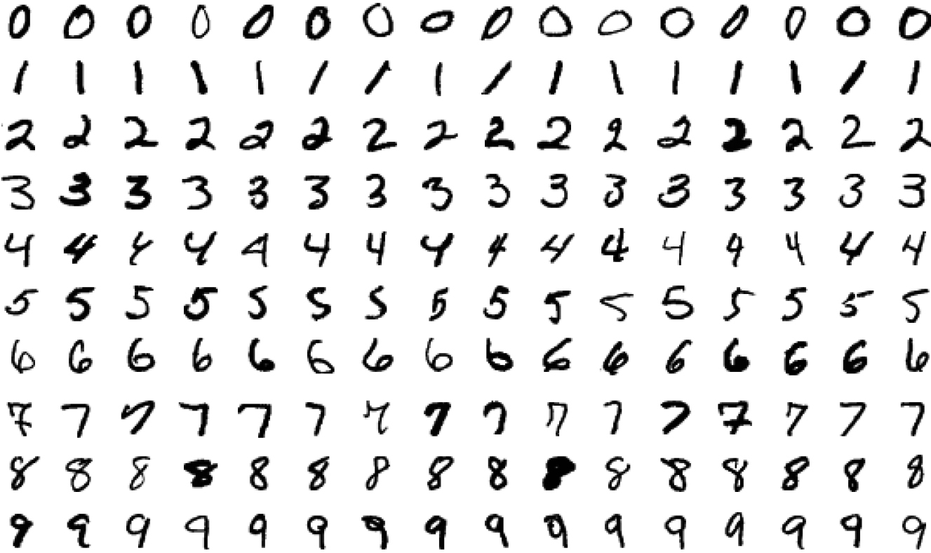
We performed evaluation of the FNNs in the image recognition task using the MNIST dataset [17], which is commonly used for training various image processing systems. It consists of handwritten digit images, $28\times 28$ pixels in size (see Fig. 4), organized into 10 classes (0 to 9) with 60,000 training and 10,000 test samples. As one can see, some examples are noisy and it is difficult to make a correct classification even for a human. Portion of training samples was used as validation data. Images were represented as vectors $\mathbf{x}_{i}\in\mathbb{R}^{784}$ , hidden layer size was fixed at 64 for all networks, and classification was done based on the softmax normalization. Mathematically, our networks perform the following computation6

⁶
Vectors are assumed to be row vectors, which are right multiplied by matrices ( $\mathbf{x}\mathbf{W}+\mathbf{b}$ ). This choice is somewhat non-standard but it maps better to the way networks are implemented in code using matrix libraries such as TensorFlow.

for a single image

\mathbf{x}\in\mathbb{R}^{784}

$\displaystyle\mathbf{h}=f(\mathbf{x}),\quad\quad\ \ \ \ \mathbf{h}\in\mathbb{R% }^{784\times 64},$ $\displaystyle\mathbf{z}=\mathbf{h}\mathbf{W}+\mathbf{b},\quad\mathbf{W}\in% \mathbb{R}^{64\times 10},\mathbf{b}\in\mathbb{R}^{10}$ $\displaystyle\hat{\mathbf{y}}=\operatorname{softmax}(\mathbf{z}),$

where $f\in\{f_{\text{GW}},f_{\text{S}},f_{\text{L}}\}$ is one of the FNNs from Section 4. Training was performed with Adam optimizer (Algorithm 5.1). We used the cross-entropy loss

$\displaystyle-{\frac{1}{n}}\sum_{i=1}^{n}\langle\mathbf{y}_{i},\log(\hat{% \mathbf{y}}_{i})\rangle,$

where $\mathbf{y}_{i}\in\mathbb{R}^{10}$ is a one-hot vector that represents the true label for the $i^{\text{th}}$ image, and $\log(\cdot)$ is applied elementwise to the predicted distribution $\hat{\mathbf{y}}_{i}\in\mathbb{R}^{10}$ . We used batches of size 100. Learning rate was tuned separately for each model on the validation data. Table 2 compares classification accuracy obtained by the models.

Table 1

Evaluation of the networks on MNIST data

Model	Accuracy	Learning rate
Vanilla feedforward NN	0.9648	0.0096
FNN of [10]	0.9695	0.0045
FNN of [27]	0.9659	0.0134
FNN of [20]	0.9638	0.0034

Figure 4.

Sample images from MNIST dataset.

As we can see, all the networks demonstrate similar performance in this task. In fact, the differences between accuracy results are not significant across the models, Pearson’s Chi-square test of independence $\chi^{2}_{3}=$ 5.6449, $p$ -value $>$ 0.1.

5.3 Language modeling

Recurrent neural networks (RNN) have demonstrated tremendous success in sequence modeling in general and in language modeling in particular. The most basic RNN [8] suffers from the problem of vanishing and exploding gradients [5] and is hard to train efficiently. One of the most widespread and efficient alternatives to the basic RNN is the Long-Short Term Memory (LSTM) model [13], which effectively addresses the problem of vanishing gradients. However, LSTM is a fairly complex model with excessive number of parameters and its inner functionality is not obvious. This complexity has motivated some of the researchers to find more apparent and less complex alternatives. One of such alternative models is a Structurally Constrained Recurrent Network (SCRN) proposed by Mikolov et al.[23]. They encouraged some of the hidden units to change their state slowly by making part of the recurrent weight matrix close to identity, thus forming a kind of longer term memory and showed that their SCRN model can outperform the simple RNN and achieve the performance comparable with the LSTM under no regularization and small parameter budget. Below we specify the SCRN-based neural language model.

Figure 5.

SCRN cell.

Let $\mathcal{W}$ be a finite vocabulary of words. We assume that words have already been converted into indices. Let $\mathbf{E}\in\mathbb{R}^{|\mathcal{W}|\times d_{\mathcal{W}}}$ be an input embedding matrix for words – i.e., it is a matrix in which the $w$ th row (denoted as $\mathbf{w}$ ) corresponds to an embedding of the word $w\in\mathcal{W}$ . Based on word embeddings $\mathbf{w_{1:k}}=\mathbf{w_{1}},\ldots,\mathbf{w_{k}}$ for a sequence of words $w_{1:k}$ , the SCRN model produces two sequences of states, $\mathbf{s_{1:k}}$ and $\mathbf{h_{1:k}}$ , according to the equations

$\displaystyle\mathbf{s_{t}}=(1-\alpha)\mathbf{w_{t}}\mathbf{B}+\alpha\mathbf{s% _{t-1}},$ (20) $\displaystyle\mathbf{h_{t}}=\sigma(\mathbf{w_{t}}\mathbf{A}+\mathbf{s_{t}}% \mathbf{P}+\mathbf{h_{t-1}}\mathbf{R}),$ (21)

where $\mathbf{B}\in\mathbb{R}^{|\mathcal{W}|\times d_{s}}$ , $\mathbf{A}\in\mathbb{R}^{|\mathcal{W}|\times d_{h}}$ , $\mathbf{P}\in\mathbb{R}^{d_{s}\times d_{h}}$ , $\mathbf{R}\in\mathbb{R}^{d_{h}\times d_{h}}$ , $d_{s}$ and $d_{h}$ are dimensions of $\mathbf{s_{t}}$ and $\mathbf{h_{t}}$ , $\sigma(\cdot)$ is the logistic sigmoid function. The last couple of states $(\mathbf{s_{k}},\mathbf{h_{k}})$ is assumed to contain information on the whole sequence $w_{1:k}$ and is further used for predicting the next word $w_{k+1}$ of a sequence according to the probability distribution

$\displaystyle\Pr(w_{k+1}\mid w_{1:k})=\operatorname{softmax}(\mathbf{s_{k}}% \mathbf{U}+\mathbf{h_{k}}\mathbf{V}),$ (22)

where $\mathbf{U}\in\mathbb{R}^{d_{s}\times|\mathcal{W}|}$ and $\mathbf{V}\in\mathbb{R}^{d_{h}\times|\mathcal{W}|}$ are output embedding matrices. For the sake of simplicity we omit bias terms in Eqs (21) and (22). Being conceptually much simpler (Fig. 5), the SCRN architecture demonstrates performance comparable to the widely used LSTM model in language modeling task [15], and this is why we chose it for our experiments.

We train and evaluate the SCRN model for $(d_{h},d_{s})$ $\in$ {(40, 10), (90, 10), (100, 40), (300, 40)} on the PTB [21] data set, for which the standard training (0–20), validation (21–22), and test (23–24) splits along with pre-processing per Mikolov et al.[24] is utilized. The PTB data is based on texts from the Wall Street Journal, and thus it is a clean dataset with no particular noise. We replace $\sigma$ in Eq. (21) with $\sigma_{\text{GW}}$ , $\sigma_{\text{S}}$ , and $\sigma_{\text{L}}$ defined in Section 4, and we refer to such modification as Fourier layers. The choice of hyperparameters is guided by the work of Kabdolov et al.[15], except that for the Fourier layers we additionally tune the learning rate, its decay schedule and the initialization scale over the validation split.7

⁷

Our SCRN implementation is available at https://github.com/zh3nis/scrn.

To evaluate the performance of the language models we use perplexity (PPL) over the test set

w_{1:T}=w_{1},\ldots,w_{T}

$\displaystyle\text{PPL}:=-\frac{1}{T}\sum_{k=1}^{T}\log\Pr(w_{k}\mid w_{1:k-1}).$

The results are provided in Table 2. As one can see, the conventional sigmoid activation outperforms all Fourier activations, and, as in the case of synthetic data, the Fourier layer of [10] is better than other Fourier layers for most of the architectures.

Table 2

Evaluation of the SCRN language models on the PTB data. Results are in perplexities of the test set, the lower the better. Columns 2–5 correspond to different configurations of the hidden ( $d_{h}$ ) and context ( $d_{s}$ ) states sizes

Activation	(40, 10)	(90, 10)	(100, 40)	(300, 40)
$\sigma$	128.0	118.6	118.7	120.6
$\sigma_{\text{GW}}$	132.8	119.6	120.1	127.9
$\sigma_{\text{S}}$	144.4	133.4	127.7	125.9
$\sigma_{\text{L}}$	165.7	139.3	147.5	156.8

6. Discussion

Why do the FNNs of Silvescu[27] and of Liu [20] underperform the one of Gallant and White [10]? These FNNs have non-sigmoidal activations, which makes their optimization more difficult. As was mentioned in Section 4, the convergence guarantees of [4] are not applicable to these models, thus it is not clear whether they can compete with the sigmoidal networks in terms of approximation errors. We will investigate the convergence rates of these FNNs analytically in our future work.

Why does the FNN of Gallant and White [10] underperform the vanilla feedforward network? Although the activation function of $f_{\text{GW}}(\cdot)$ is sigmoidal, it still underperforms the standard feedforward neural network in almost all cases. We hypothesize that this is because $\sigma_{\text{GW}}$ is constant outside $\left[-\frac{\pi}{2},\frac{\pi}{2}\right]$ , while $\sigma(x)=1/(1+e^{-x})$ is never constant. This means that $\forall x_{1},\,x_{2}\in(\pi/2,\infty)$ : $\sigma_{\text{GW}}(x_{1})=\sigma_{\text{GW}}(x_{2})$ , i.e. the activation of Gallant and White[10] Eq. (3) does not distinguish between any values to the right from $\pi/2$ (and to the left from $-\pi/2$ ). The standard sigmoid activation $\sigma(\cdot)$ , on the other hand, can theoretically8

⁸
In practice, when implemented on a computer $\sigma(\cdot)$ will also be “constant” outside an interval $[-a,a]$ , where $a$ depends on the type of precision used for computations.

distinguish between any pair

x_{1},\,x_{2}\in\mathbb{R}

x_{1}\neq x_{2}

. To see whether the constant behavior of

\sigma_{\text{GW}}

indeed causes problems, we look at the pre-activated values

x\cdot w+b

for

x

from the validation split in the synthetic task of approximating

x\mapsto|x|

x\in[-\pi,\pi]

. The histogram of these pre-activated values for the

f_{\text{GW}}

with hidden layer size

n=

100 is given in Fig. 6.

Figure 6.

Histogram of pre-activated values ( $x\cdot w+b$ ) in the FNN of Gallant and White [10]. Frequencies are at log-scale.

It turns out that $\approx$ 8% of pre-activated values are outside of $[-\pi/2,\pi/2]$ , and this information is lost when filtered through $\sigma_{\text{GW}}$ .

7. Conclusion and future work

All Fourier neural networks are not better than the standard neural network with sigmoid activation except when it comes to modeling synthetic data. The architecture of [10] is the best among Fourier neural networks. When the function being approximated is known and depends on multiple variables, the neural networks with just one hidden layer may provide much better approximation compared to truncated Fourier series.

In this paper we focused on neural architectures with one hidden layer. It is interesting to compare Fourier neural networks in a multilayer setup. We defer such study to our future work which will also include experiments with a larger variety of functions, as well as mathematical analysis of the approximation of Barron functions by Silvescu’s and Liu’s Fourier neural networks.

Footnotes

Acknowledgments

This work has been supported by the Committee of Science of the Ministry of Education and Science of the Republic of Kazakhstan, IRN AP05133700.

References

Abadi

Barham

Chen

Davis

Dean

Devin

Ghemawat

Irving

Isard

et al., Tensorflow: A system for large-scale machine learning, In OSDI, volume 16, 2016, pp. 265–283.

Alimov

S.A.

Il’in

V.A.

and Nikishin

E.M.

, Convergence problems of multiple trigonometric series and spectral decompositions, Russian Mathematical Surveys 31(6) (1976), 29.

Alimov

S.A.

Il’in

V.A.

and Nikishin

E.M.

, Problems of convergence of multiple trigonometric series and spectral decompositions, Russian Mathematical Surveys 32(1) (1977), 115–139.

Barron

A.R.

, Universal approximation bounds for superpositions of a sigmoidal function, IEEE Transactions on Information Theory 39(3) (1993), 930–945.

Bengio

Simard

and Frasconi

, Learning long-term dependencies with gradient descent is difficult, IEEE Transactions on Neural Networks 5(2) (1994), 157–166.

Bishop

C.M.

, Pattern recognition and machine learning, springer, 2006.

Cybenko

, Approximation by superpositions of a sigmoidal function, Mathematics of Control, Signals and Systems 2(4) (1989), 303–314.

Elman

J.L.

, Finding structure in time, Cognitive Science 14(2) (1990), 179–211.

Folland

G.B.

, Fourier analysis and its applications, volume 4. American Mathematical Soc., 1992.

10.

Gallant

A.R.

and White

, There exists a neural network that does not make avoidable mistakes, In Proceedings of the Second Annual IEEE Conference on Neural Networks, San Diego, CA, I, 1988.

11.

Gatys

L.A.

Ecker

A.S.

and Bethge

, A neural algorithm of artistic style, arXiv preprint arXiv:1508.06576, 2015.

12.

Götze

, Lattice point problems and values of quadratic forms, Inventiones Mathematicae 157(1) (2004), 195–226.

13.

Hochreiter

and Schmidhuber

, Long short-term memory, Neural Computation 9(8) (1997), 1735–1780.

14.

Hornik

Stinchcombe

and White

, Multilayer feedforward networks are universal approximators, Neural Networks 2(5) (1989), 359–366.

15.

Kabdolov

Assylbekov

and Takhanov

, Reproducing and regularizing the scrn model, In Proc. of COLING, 2018.

16.

Kingma

D.P.

and Ba

, Adam: A method for stochastic optimization, In Proceedings of ICLR, 2015.

17.

LeCun

Bottou

Bengio

and Haffner

, Gradient-based learning applied to document recognition, Proceedings of the IEEE 86(11) (1998), 2278–2324.

18.

Lee

Risteski

and Arora

, On the ability of neural nets to express distributions, In Conference on Learning Theory, 2017, pp. 1271–1296.

19.

Leshno

Lin

V.Y.

Pinkus

and Schocken

, Multilayer feedforward networks with a nonpolynomial activation function can approximate any function, Neural Networks 6(6) (1993), 861–867.

20.

Liu

, Fourier neural network for machine learning, In Machine Learning and Cybernetics (ICMLC), 2013 International Conference on, volume 1, IEEE, 2013, pp. 285–290.

21.

Marcus

M.P.

Marcinkiewicz

M.A.

and Santorini

, Building a large annotated corpus of english: The penn treebank, Computational Linguistics 19(2) (1993), 313–330.

22.

McCaffrey

D.F.

and Gallant

A.R.

, Convergence rates for single hidden layer feedforward networks, Neural Networks 7(1) (1994), 147–158.

23.

Mikolov

Joulin

Chopra

Mathieu

and Ranzato

, Learning longer memory in recurrent neural networks, In Proc. of ICLR Workshop Track, 2015.

24.

Mikolov

Karafiát

Burget

Cernockỳ

and Khudanpur

, Recurrent neural network based language model, In Proc. of INTERSPEECH, 2010.

25.

Pinsky

M.A.

Stanton

N.K.

and Trapa

P.E.

, Fourier series of radial functions in several variables, Journal of Functional Analysis 116(1) (1993), 111–132.

26.

Samuel

A.L.

, Some studies in machine learning using the game of checkers, IBM Journal of Research and Development, 1959, pp. 71–105.

27.

Silvescu

, Fourier neural networks, In Neural Networks, 1999. IJCNN’99. International Joint Conference on, volume 1, IEEE, 1999, pp. 488–491.

28.

Tan

, Fourier neural networks and generalized single hidden layer networks in aircraft engine fault diagnostics, Journal of Engineering for Gas Turbines and Power 128(4) (2006), 773–782.

29.

Zuo

and Cai

, Tracking control of nonlinear systems using fourier neural network, In Advanced Intelligent Mechatronics, Proceedings, 2005 IEEE/ASME International Conference on, IEEE, 2005, pp. 670–675.

30.

Zuo

and Cai

, Adaptive-fourier-neural-network-based control for a class of uncertain nonlinear systems, IEEE Transactions on Neural Networks 19(10) (2008), 1689–1701.

31.

Zuo

Zhu

and Cai

, Fourier-neural-network-based learning control for a class of nonlinear systems with flexible components, IEEE Transactions on Neural Networks 20(1) (2009), 139–151.

Fourier neural networks: A comparative study

Abstract

Keywords

1. Introduction

3. Preliminaries

2 I.e. we put σ ⁢ ( x ) := 1 1 + exp ⁡ ( - x ) in Eq. (1).

3 This means that 𝕀 [ ∥ 𝐱 ∥ ⩽ 1 ] = 1 if ∥ 𝐱 ∥ ⩽ 1 , and 0 otherwise.

.

Proof..

.

Proof..

6 Vectors are assumed to be row vectors, which are right multiplied by matrices ( 𝐱𝐖 + 𝐛 ). This choice is somewhat non-standard but it maps better to the way networks are implemented in code using matrix libraries such as TensorFlow.

8 In practice, when implemented on a computer σ ⁢ ( ⋅ ) will also be “constant” outside an interval [ - a , a ] , where a depends on the type of precision used for computations.

Footnotes

Acknowledgments

References

²
I.e. we put $\sigma(x):=\frac{1}{1+\exp(-x)}$ in Eq. (1).

³
This means that $\mathbb{I}[\|\mathbf{x}\|\leqslant 1]=1$ if $\|\mathbf{x}\|\leqslant 1$ , and 0 otherwise.

⁶
Vectors are assumed to be row vectors, which are right multiplied by matrices ( $\mathbf{x}\mathbf{W}+\mathbf{b}$ ). This choice is somewhat non-standard but it maps better to the way networks are implemented in code using matrix libraries such as TensorFlow.

⁸
In practice, when implemented on a computer $\sigma(\cdot)$ will also be “constant” outside an interval $[-a,a]$ , where $a$ depends on the type of precision used for computations.