The lack of annotated data is one of the major barriers facing machine learning applications today. Learning from crowds, i.e. collecting ground-truth data from multiple inexpensive annotators, has become a common method to cope with this issue. It has been recently shown that modeling the varying quality of the annotations obtained in this way, is fundamental to obtain satisfactory performance in tasks where inexpert annotators may represent the majority but not the most trusted group. Unfortunately, existing techniques represent annotation patterns for each annotator individually, making the models difficult to estimate in large-scale scenarios.
In this paper, we present two models to address these problems. Both methods are based on the hypothesis that it is possible to learn collective annotation patterns by introducing confusion matrices that involve groups of data point annotations or annotators. The first approach clusters data points with a common annotation pattern, regardless the annotators from which the labels have been obtained. Implicitly, this method attributes annotation mistakes to the complexity of the data itself and not to the variable behavior of the annotators. The second approach explicitly maps annotators to latent groups that are collectively parametrized to learn a common annotation pattern. Our experimental results show that, compared with other methods for learning from crowds, both methods have advantages in scenarios with a large number of annotators and a small number of annotations per annotator.
Currently, artificial intelligence methods for analyzing and organizing data have been widely spread into several areas of science and industry. Many of these applications rely on supervised learning, i.e., methods able to learn an input-output mapping from large amounts of data (inputs) explicitly annotated with ground-truth labels (outputs). However, in many real-world tasks, obtaining accurate labels can be difficult and time-consuming. For instance, in biomedical imaging analysis, ground-truth labels indicating a clinical condition of interest could only be obtained after slow and expensive procedures in physical labs. On the other hand, collecting multiple subjective but possibly inaccurate labels from annotators of different levels of expertise is often more feasible and cheaper [1]. Current crowd-sourcing platforms such as Amazon Mechanical Turk1
are making this procedure very popular [2], especially in computer vision and natural language processing.
Learning from crowds refers to the scenario in which multiple users, termed annotators, jointly provide annotations for the different items in a database. Often, the quality of these annotations is unknown apriori and can also vary depending on the annotator, the complexity of the annotation task, or the difficulty of certain data points. In particular, inaccurate annotations may come from inexpert contributors, spammers looking for easy money, or even malicious users interested in providing false evaluations. Consequently, training a traditional supervised model, with annotations collected from crowds, is often ineffective. Similarly, simple aggregation rules such as majority voting, which reduce crowd annotations to a single label, can fail if the expertise of the different annotators varies significantly [3] or if, as usual in crowd-sourcing platforms, there are many items annotated by a small subset of contributors. These drawbacks call for methods that improve the accuracy of models trained on crowd-sourced data.
The problem of learning from annotations of varying reliability can be traced back to [4]. Here, Dawid and Skene proposed a method, based on the EM algorithm, that automatically detects the annotation pattern of each contributor using a confusion matrix. It estimates a consensus label that can be used to train a standard classifier in a second phase. Many subsequent methods are extensions of this framework. For instance, Zhang et al. [5] and Sinha et al. [6] proposed different ways to speed up the convergence of the method. Raykar et al. [7] proposed to directly train a ground-truth predictor in the maximization step of the EM algorithm without the second phase. Kajino et al. [8] presented an algorithm that trains a separate model for each annotator and then infers a consensus model rather than a consensus label. More recently, Albarqouni et al. [9] proposed the use of deep learning to implement the ground-truth predictor of the approaches presented in [7, 10]. Encoding the confusion matrices into a neural net consents the use of simpler training procedures based on the back-propagation to learn the parameters.
A common limitation of the current models is that the number of learnable parameters becomes very large as the number of annotators increases, therefore limiting their inference and computational scalability to massive crowd-sourcing scenarios. In this paper, we present two methods to address this problem. We note that a limiting factor of current methods is that they represent labeling patterns for each annotator independently. Our methods depart from this general rule by learning collective annotation patterns, represented as latent confusion matrices that involve groups of data points or annotations. The first approach assumes that annotated data has been generated from a mixture of confusion matrices following a process that is conditionally independent of the annotators providing the labels. Implicitly, this approach attributes annotation mistakes to the complexity of the data itself and not to the varying behavior of the annotators. The second approach instead, explicitly clusters annotators, by modeling the confusion matrix involved in an annotation as a latent variable whose distribution depends on the user providing the label. In contrast to previous approaches, our models have a fixed and small number of components that make estimation more reliable in scenarios with a large number of annotators but a varying number of contributions per instance.
Experiments results over synthetic, semi-synthetic and real data, confirm that the proposed methods can scale better (in terms of memory consumption and time) to large-scale crowd-sourcing scenarios. Also, they outperform the state-of-the-art methods in scenarios in which a relatively small number of annotations per item is available. In particular, one of the methods naturally adapts to the situation in which the contributors are unknown (anonymous) and thus it is not possible to identify the source of the annotations. Besides assessing and comparing the models using standard metrics, we qualitatively analyze the groups found by the models in real datasets, to determine the degree to which a human can understand the underlying patterns.
This work is an extension of a shorter research presented in [11]. The additional contributions can be summarized as follows:
The literature review has been extended.
Besides the original method (CMM), a second method termed C-MoA is proposed. As discussed above, the novel method does not cluster annotations but annotators. Also, pseudo-codes are presented to clarify the differences.
The experimental setting is expanded by adding a second public and real dataset from the text domain which is large enough to train deep learning models.
A qualitative analysis of the clusters found by the methods is presented.
The comparison focused on the scalability of the proposed methods and baselines is re-organized to provide a more detailed analysis.
The remainder of this paper is organized as follows: Section 2 formalizes the problem and introduces the notation used for the proposed methods, which are presented in Section 3. Section 4 provides a comprehensive discussion of the related work. In Section 5, the proposed models are experimentally assessed and compared with baseline methods. Finally, Section 6 summarizes the conclusions of this work.
Background
Consider an input pattern observed with probability distribution and a ground-truth label observed with conditional probability distribution . The goal of a supervised learning algorithm is to estimate statistics of from a set of examples , where . More specifically, given a loss function and a hypothesis space , a supervised learning algorithm tries to minimize in when is unknown and only a finite sample is given. For instance, if , as in pattern recognition, the goal is equivalent to approximate the mode of . If , the goal is to estimate the mean of .
In learning from crowds, the goal is the same, but the ground-truth labels corresponding to the input patterns are not observed. Instead, for each training pattern , multiple noisy labels , with are given. These labels have been collected from annotators and do not follow the ground-truth distribution . Instead, they are generated from an unknown process that represents the “ability” or “expertise” of the annotators.
In general, the annotations for a pattern come from a subset of the set of all the annotators participating in the labelling process. We can distinguish two scenarios depending on how different are the number of annotations of each example . The simpler case is when , which is termed densescenario in the rest of this paper. In the second scenario, termed sparse scenario, the number of labels collected by data point and annotator vary, i.e. . Furthermore, we also are interested in a case, referred to as the Global scenario, in which we are given , but we do not know which annotators provided the labels i.e., we know but not . The opposite scenario, named as Individual, allows to study the properties of each annotator separately.
Focus. In this work, we study the pattern recognition case, that is, we let be a small set of categories or classes .
Performance Evaluation. The performance of a system designed for the crowd-sourcing scenario is measured through the quality to estimate the unobserved ground truth. The classic setting corresponds to the situation in which we have multiple annotations for learning on the train set and a trusted ground truth3
A unique label that is assumed has no errors.
available for evaluation on the test set.
Proposed methods
In this section we propose two learning from crowds methods with the objective of cluster/group similar behavior, specifically labeling mistakes patterns. Both proposed method use the following model basis of latent/hidden variables.
Models basis
In order to explain an annotation , assigned to an input pattern , we propose a finite mixture model (MM) [12] of the form
where is a categorical random variable with values in identifying the group/ component that generated the observation , while is one of the possible sub-models that represent different annotation patterns that can occur in the labelling process. The objective of introducing this latent variable into the annotation process it is for group annotations or annotator that follow a similar rules to annotate data or for which similar mistakes were made.
As in previous works, we represent the ground-truth label as a latent/hidden variable with (unknown) probability distribution and values in . Thereby, the relationship between an annotation and the ground-truth for is obtained as follows
where is the number of classes and the second line was obtained by assuming that is conditionally independent of given , in order to keep a simpler model. Indeed, this simplification allow us to parametrize the component using only parameters (confusion matrix) per sub-model (group), as Table 1 summarized. Besides, it is assumed that the ground truth is conditional independent of the groups given the input patterns , and is modeled as a single predictive model that approximates the ground-truth distribution .
Model specification: CMM
We start by proposing a model and a data representation that full-fills the requirements of the Global scenario defined in Section 4. The Global scenario allow us to handle naturally the sparse annotations scenario, i.e. variable number of annotations per input pattern and annotators. As we do not know the annotators identity on this scenario, we assumed the existence of annotations groups. Substituting Eq. (2) into Eq. (1), we obtain the specification of the proposed Crowd Mixture Model (CMM) for annotation
here, represent an a-priori probability that pattern is annotated according to the behavior of group , this value could be seen as the mixing coefficient of a mixture model over the annotations. Note that we are assuming that the mixing coefficients are independent of . If we relax this assumption, we obtain a mixture of experts model (MoE) with gating functions . The motivation to consider a GMM instead of a MoE is just to keep a simple model with small number of learnable parameters.
We define an annotation representation as a -dimensional vector whose components are the frequencies of label among the annotations of a pattern . If we assume that those annotations are conditionally independent given , we obtain that follows a Multinomial distribution with sample size and probabilities given by the model parametrization (see Table 1) on Eq. (3). The conditional log-likelihood of the data is thus given by
The model parameters can be learnt to maximize . Unfortunately, due to the log-sum in the objective, this optimization is not straightforward. We address this issue using the EM algorithm [13].
Training procedure
Considering the Jensen inequality, we can consider any bi-variate distribution assigning annotations among groups and ground-truth categories, to obtain the following lower bound of
The EM algorithm [14] now follows easily. In one step, we improve our estimate of to make the bound tight. Then, we optimize the lower bound in the model parameters . The iteration of these two steps is guaranteed to converge to a local maximum of . In practice multiple restarts with different initializations can mitigate the local maximum problem. A pseudo-code to illustrate the optimization of this method is presented in Algorithm 1, where SGD on line 9 stands for the stochastic gradient descend method to optimize neural nets model. In addition, the exact solutions are provided below.
Method CMM (EM)[1] – input patterns () – global annotations () – number of groups to model – modeled parameters Initialize tuple embedding using data , according to (10) -means // Initialize using (, ), based on (9) // Maximization step Update using current estimate and data , based on the solution (7-a) Update using current estimate and data , based on the solution (7-b) Update using current estimate and data , through SGD on (8) // Expectation step Update estimation, with data and parameters , based on (6) Calculate based on (4) convergence under some criteria
E-step. For grouping the annotations based on ground-truth, we obtain
M-step. For the mixing coefficients and confusion matrices, we obtain
where is the marginal probability of groups for every , then confusion matrix is a weighted average of annotations belonging that group. Now, for the neural net model the following objective has to be minimize:
where is a marginal probability, and is the categorical cross-entropy between the neural net and a “consensus” distribution on the categories, , which has been computed for considering the current estimation and observed annotations.
The initialization of the E-step is expressed through the approximation
with the Majority Voting probabilities (soft-MV) of all annotations for that pattern , while for a clustering is performed with K-means to get hard-labels assignment. The clustering is based on a representation of the tuple , given by
with a one-hot vector with a one on position , and a distance function among vectors, , with the Hadamard product. The representation gives a value for every every annotation based on the only a-priori information that pattern has, majority opinion.
Summary of the assumptions made by both models. Besides, the components parametrization is presented and the number of trainable parameters. A restriction of the modeling is that they are valid probabilities (sum 1), which reduces the free parameters in some cases. C-MoA method use a non-trainable embedding layer into that project to a -dimensional vector. CMM, C-MoA
Probability
Assumption
Description
Model of the component
# Parameters
Confusion matrix or ability of each group
Cube of learnable parameters:
Predictive model of the ground truth
Neural net (DL model):
Mixing coefficient over annotations
Vector of learnable parameters:
Mixing gate function over annotators
MLP-1 (one hidden layer of units without bias):
Model specification: C-MoA
The idea of work under the same conditions of classic learning from crowds, we proposed a model that full-fills the requirements of the Individual scenario. On this case, as we know the annotators identity, we assume the existence of annotators groups. In order to adapt the Individual scenario to handle sparse annotations, we introduce a new variable: , with and . The variable contains the the information (identifier) of the annotator that generated the annotations from input pattern . Furthermore, it allows to have variable number of annotaions per data and avoid the common assumption of the dense scenario. Based on this, substituting Eq. (2) into Eq. (1), allow us to obtain the specification of the proposed Crowd-Mixture of Annotator (C-MoA) model for annotation
here it can be seen other of the main differences regarding the CMM model (contrasting to Eq. (3)): the groups probability is assumed to be conditional independent of the input pattern , showing a similarity to a mixture of expert (MoE) model associated to the annotators , with gating function . As Table 1 shows, this gating function is modeled with a neural net . Besides, the annotations of each group4
The value is expressed as a one-hot vector, where represent the value in position of a -dimensional vector, with possibles values 0 or 1.
are assumed independent given the group and ground truth , following a Multinomial distribution
Extending the previous idea, if we assume that every observed annotation is conditional independent of other annotations given the input pattern and annotators identity, we obtain that the conditional log-likelihood for the data given the model parametrization (see Table 1) on Eq. (3) is given by
Method C-MoA (EM)[1] – input patterns () – individual annotations () – annotators identity () – number of groups to model – modeled parameters Initialize annotators embedding using , based on (21) // -means Set to annotators in , using // Initialize using , , based on (20) // Maximization step Update using current estimate and data , based on the solution (17) Update using current estimate and data , through SGD on (18) Update using current estimate and data , through SGD on (19) // Expectation step Update estimation with data and parameters , based on (16) Calculate based on (14) convergence under some criteria
This model parameters , similar to Eq. (4) has a log-sum in the objective that need to be correctly handled. We address this issue using the EM algorithm [14].
Training procedure
Similar to the CMM method, we consider a bi-variate distribution and the Jensen inequality to obtain the following lower bound of
Based on this lower bound, the EM algorithm is applied. A pseudo-code to illustrate the optimization of this method is presented in Algorithm 2, where SGD on lines 9 and 10 stands for the stochastic gradient descend method to optimize neural nets model, and the generated solutions are provided below.
E-step. For grouping the annotations based on ground-truth, we obtain
with the normalization constant over and for every .
M-step. For the confusion matrices the solution is quite similar to CMM method, and given by
Now, for the gating function model the following objective has to be minimize:
with the marginal probability and is the categorical cross-entropy between the gating model and the auxiliary distribution. Also, defining the marginal probability we obtain the objective to minimize for the neural net model:
now represent the “consensus” distribution of classes over all annotations computed for , considering the current estimation estimation.
The initialization of the E-step is expressed through the approximation
with the Majority Voting probabilities (soft-MV) of all annotations for that pattern , while for a clustering is performed with K-means to get hard-labels assignment. The clustering is based on a vector representation, , of the annotators, , that is also used as an non-learnable embedding layer on the model, as Table 1 describe.
Annotators representation
Defining , as the set of all the annotations generated from the -th annotator, the vector representation (embedding) is build as:
This representation is generating according to the number of times that every class is repeated from an annotator, , storing information from the possible bias that an annotator has, .
As Table 1 shows, the number of trainable parameters for the model is given based on this simplified representation of annotators with dimensions. As this representation is non-learnable, it does not affect the inference complexity, but the consumption memory as the results on following section showw. Also, it allows a representation for annotators, or a set of annotations, even outside the training data.
Methods discussion
The two proposed methods have the same objective but achieved in different ways. The main difference is the data representation or scenario setting (Global and Individual), that carried other discrepancies. It can be seen that the CMM model does a desegregation or decomposition of all the observed annotations for every data, defining the groups/component on it. Otherwise, the C-MoA method does an annotators assignment to the groups/components based on her behavior labeling the data.
The Table 1 shows the assumptions on the modeled components and shows that the only difference here is respect to the groups, besides of its associated parameters. Simplification of all the assumptions made generate two models with learnable parameters independent to the number of annotators . Indeed, excluding (as every proposed method should has), the total parameters of both methods5
C-MoA model should be , but is usually modeled smaller than , so it keeps the expression .
are . Thus, the complexity will only depend on the number of components/groups to model ().
Confusion matrix assignment
As our models do not have explicitly a confusion matrix per annotator we need an estimation based on the modeled components. The individual confusion matrix of an annotator can be estimate as
where the estimation is a weighted average of the modeled confusion matrices, using the probabilities as weights. However, our CMM method does not have this probability explicitly, so it needs a group assignment derivation.
Given any set of annotations for a pattern , we can compute the probability that these annotations were generated by the component in the CMM model as
The probability that an annotator belongs to the group can be estimated with all her annotations. This expression allows to cluster annotations and annotators, even outside the training data.
Related work
Existing methods for learning from crowds can be grouped in four categories: (i) simple aggregation methods, (ii) methods without predictive model, (iii) methods with predictive model, and (iv) deep learning methods.
Simple aggregation methods
These methods address the crowd-sourcing problem by reducing the multiple annotations to a single target for each input pattern . The goal is to define a ground truth as a function of the annotations , and thus return to the classic supervised scenario of learning a predictive model to approximate the map . Here, the function is usually a summary statistic such as the mean, the median or the mode.
The most used technique in this category, probably due to its simplicity and speed, corresponds to Majority Voting (MV) [15]. This technique can be categorized as a solution to the sparse global scenario because it does not need to know the source of the annotations. The method has two versions for classification settings [16]:
Hard-MV: Here, a point estimate of the ground truth label is obtained as the majority annotation among the categories for each example, that is, is the function that computes the mode of the labels in :
Soft-MV: In this case, the ground truth is represented as a probability distribution among the categories and is obtained by computing the relative frequency of each class among the annotations observed for each example, that is,
As MV methods give the same weight to the different annotations, they implicitly assume that all the annotators have the same ability and for all data equally. However, this assumption is not realistic since annotators may not be uniformly skilled or they may have a bias to solve certain tasks. For this reason, MV methods have shown limited performance when annotators have varying levels of expertise or in cases where there are only few annotations per data point [3].
Methods without predictive methods
These techniques also reduce multiple annotations to a single final label to train a traditional supervised model in a separate step. However, they implement more specialized techniques to deal with the different abilities of the annotators. Specifically, the graphical model for the problem is built with the assumption that we do not have access to the input pattern, i.e, . Furthermore, these works focus on the dense individual setting (), and hence refers simultaneously to the annotation and annotator.
Dawid and Skene (D&S) presented in [4] the first method that uses a probabilistic model to solve the learning problem with multiple annotations. The authors assume that the ability of each annotator is independent of the input pattern, that is, . The probability that an annotator provides a certain annotation given that the ground truth for the input pattern is is represented with a confusion matrix . The ground truth is represented as a latent variable whose distribution can be inferred using the EM algorithm. This method initializes using soft-MV and then iterates until convergence the following two steps:
step: the maximum likelihood estimators of the confusion matrices are obtained as if the ground truth distributions had been found. In a similar way, the estimation of the marginals is updated.
step: the estimation of the ground truth distribution for each training item is improved, based on the observed annotations in . These are weighted considering the probability of each labels, which is obtained from the confusion matrix and the marginals .
As the D&S model uses different parameters for each training point, it obtains closed solutions for each step of the EM algorithm. Given a number of fixed iterations, and under the same initialization, it produces the same final solution. However, for the same reason above, it has no way to estimate the ground truth of novel data. Smyth et al. propose in [17] an out-of-sample extension the D&S model based on training a predictive model on the inferred ground truth. The method was successfully applied to volcano detection on radio images of Venus. More recently in 2016, Zhang et al. propose in [5] a new way to initialize the optimization of the D&S model without using soft-MV. This work uses a spectral tensor decomposition of the annotations to accelerate the convergence of the EM algorithm to the local optimum. However, the method is quite complex and costly in terms of computational memory at initialization. In 2018, Sinha et al. [6] also propose a way to accelerate the convergence (reduce the number of iterations) of the EM algorithm. They empirically modify the estimation of the latent variable to its hard version, i.e. at each iteration, is replaced by a vector of zeros expect for dimension that is set to 1.
For binary classification, Whitehill et al. [18] consider the difficulty of an input pattern for being correctly labeled. To do that, they model the labeling probability with two parameters: (i) the expertise of each annotator , and (ii) the difficulty of the input pattern . In this way, the authors propose an explicit probabilistic model based on these two parameters: . The ground truth is also modeled as a latent variable, with distribution , while the inference and optimization of all the variables is performed in the same way as the D&S model, i.e. using the EM algorithm.
The method proposed by Zhou et al. in [19] also represents the annotator ability using a confusion matrix, but it changes the problem formulation to be optiized in another way. The model is optimized with the minimax of the entropy of the confusion, given the annotations and the ground truth. However, the resolution involves two iterative steps, that they cannot obtain in a closed way, as is the case with the D&S model. In one step they estimate the ground truth as usual. However, in the second step, they need to optimize the parameters in the confusion matrices with gradient descent.
The main disadvantage of the works from this category is the assumption of independence or lack of access of the probabilistic model to the input patterns, which ends up making it easier model fit, but at the same time avoids recognizing data behavior that could help inference and learning.
Methods with predictive methods
These methods include the predictive model of ground truth inside the problem formulation. Thus, they avoid the second learning stage of the algorithms from the previous category. As a consequence, it allows the model to learn labeling patterns that depend on , being the main advantage. For example, allow the model detects the characteristics or intrinsic noise that make it confusing the labeling process of input patterns. The works presented in this section focus on binary classification , that is, the label space is while is modeled with a logistic regression of learning, .
Raykar et al. [7] propose the first work to include the predictive model into the formulatio. This work extends the D&S model considering that in the binary case there are only two free parameters per matrix: The first one, is the parameter , called sensitivity (true positive rate), and the other is , called specificity (1-false positive rate). Next, the probabilistic model that relates the variables is factorized as:
where the independence of the annotations given the ground truth is assumed. That is, . Furthermore, this express how likely is to observe the annotations given each possible ground truth label and is modeled as
The EM algorithm is used to obtain the parameter. Experimental results show that this approach provides a good estimation of the ground truth with noisy labels.
Yan et al. [20] propose a more general model that assume that the ability of the annotator depends on the input pattern. The expertise of each annotator for an input pattern is modeled by a function , while an explicit model is defined for the ability , centered on the ground truth that varies on the basis of this annotator’s expertise on the input pattern, given by:
The ground truth inference and optimization of the parameters involved is done using the EM algorithm, similar to the Raykar et al. method [7]. Kajino et al. [8] present a convex model for learning multiple annotations avoiding the use of the EM algorithm. This work defines a predictive model for the ground truth with normal distributed parameters over a prior . In addition, and similar to Yan et al. [20], it adds a logistic regression model for each annotator to model the ability, . The parameters of each annotator model is centered at the base: . While the dispersion parameters and are manually set. Next, it is optimized with a two steps iterative method with an experimental advantage over EM algorithm, by having a lower variance on the solutions obtained. The problem of these proposals is that they present one model per annotator, which considerable increase the parameters (more complex). Besides, on Kajino et al. proposal, the predictive model of ground truth is defined by the majority, a strong assumption for crowdsourcing problems.
Rodrigues et al. [16] present a simplification of the current models. The proposal modeled the ability of the annotators for an input pattern using a binary representation which is named reliability. It is set to 1 when the annotator has an expert behavior and 0 when it has a random behavior. In this way the model of ability is expressed as:
where , which is model as , and . For each annotator, a binary model decides between these two extreme types of behavior. The proposed final model has the parameters associated with the predictor model, , and the parameters for the ability model . This model is inferred and optimized with the EM algorithm. The work shows good experimental performance in estimating ground truth for sparse scenarios.
Bi et al. [21] propose a method that tries to combine all the good ideas from previous works. First, similar to Kajino et al. [8], it defines a base predictor model for the generation of the ground truth, one model for each annotator with model-centered parameters base and variability proportional to the annotator ability. Then, a soft modification on the latent variable from Rodrigues et al. [16] is made, indicating if the annotator behaves as reliable, delivering a label based on his ability, or, if he behaves randomly, delivering a fixed value without looking at the input pattern, expressed as:
with , while depends on the input pattern , on the annotator ability and its sensitivity. For inference, the EM algorithm is used which ends up with a second two-step iterative method inside the M-step. The proposal requires input patterns with a large number of annotations () and annotators that label a large amount of data, which can be quite expensive.
Deep learning methods
Recent works have explored the use of Deep Learning (DL) to implement predictive models in learning from crowdsourcing. This is, is modeled by a multi-layer neural network. The benefit of using neural network models in is that it gives the model greater flexibility to learn patterns from raw data such as images or text. Therefore, it is possible to obtain better understanding and capture the actual behavior on the labeling process of the annotators.
Albarqouni et al. [9] use a neural networks to address a breast cancer screening problem on images. The authors extend the proposal of Raykar et al. [7], replacing the logistic regression, by a convolutional network for binary classification as ground truth predictor. The objective is to predict the result that a biopsy would deliver (ground truth) from the multiple annotations that people inexperienced give over an image (exams). Guan et al. [22] also explores the crowdsourcing learning scenario for a medical problem by using convolutional neural network models. Using an approach similar to that of Kajino et al. [8] avoids the use of the EM algorithm. For this, the authors define a convolutional network with shared parameters between the annotators, this network is independently trained to imitate the annotations of each of them. Then, the ground truth is defined as a transformation of the annotators’ predictions into the neural model, using a weighted average. The objective of this second stage is based on the the following heuristic: for an input pattern, annotators who did not tag should mimic the consensus of all annotators who did tag it (Majority Voting).
Simultaneously, Rodrigues et al. [10] extend [9] to multiple classes, making minor variations to the mathematical formulation. It also presents an alternative model to obtain a predictive model over the ground truth using only backpropagation. First, a neural network is constructed to processes the input patterns where the last layer, with softmax probabilistic activation function, represents the classification on the classes, as a base model . Then, a large layer is added, called the CrowdLayer, which contains other probabilistic layers in parallel, one for each annotator, imitating the annotations given by them. The components of the final model are interpreted as: the first neural network is the predictor model of the ground truth, while the matrix parameters associated to each annotator in the CrowdLayer are the confusion matrices. The parameters of this two components are optimized jointly to reconstruct each annotation on the final layer. The work shows a slight improvement in performance on several datasets from different domains with respect to the D&S model, the Albarqouni et al. [9] multi-classes and Guan et al. [22]. Rodrigues et al. also explores a model that, instead of a matrix as parameters in the CrowdLayer has two vectors: one to scale, via component-to-component multiplication, and another to add the bias from the annotator : . Unlike the EM-based algorithms that ensure convergence to a local optimum, the proposed algorithms in this work do not ensure convergence to the values that are expected to be modeled. Because they are based on a heuristic that is optimized using stochastic optimization.
Liu et al. [23] extend the idea from Rodrigues et al. [10] by replacing the neural network that predicts the ground truth with an alternative so-called deep clustering. Unlike the ordinary clustering, it performs soft clustering on a embedding or latent representation generated by an autoencoder. As in [10], it assumes that the segmentation generated by the deep clustering on input patterns is related to the real tags. In this work, each cluster is assigned a distribution over the possible labels of the ground truth. Indeed, the ground truth of each input pattern is finally obtained through the most probable tag, given by the information from clustering and the imitation of the annotators under the CrowdLayer of Rodrigues et al. The final model, which is so-called deep clustering-based aggregation model (DCAM), combines and optimizes the deep clustering and the CrowdLayer. In comparison with [10], DCAM increases the number of parameters in the model, and its time complexity is larger because it performs a clustering during each iteration.
Discussion
As stated in [2], today there is no a single method that is superior to the others in all cases, because different assumptions must be met to achieve good results. However, algorithms that use a confusion matrix, such as our method, to represent the ability of the annotators perform experimentally better than the others [2]. However, although almost all methods focus on dense individual scenario, we propose two setups (individual and global) that naturally adapts sparse scenarios, each of them with a fixed number of components. Here, annotations and annotators can be assigned. As shown in Table 1 this makes the number of parameters independent of for each setup. In addition to computational efficiency, the grouping of annotations/annotators allows the statistical efficiency to be increased, especially in scenarios where annotators provide a small number of labels and, therefore, the estimation of confusion matrices should be done with very few annotations.
Experiments
We evaluate our method on real and simulated scenarios, comparing it against four baselines from the state-of-the-art: DL-DS [4], DL-EM ([9] and generalized in [10]), and both versions of MV [16]: hardMV and softMV. We also include the upper bound performance of a model trained with the ground-truth, referred to as Ideal. In the vein of latest works, all the methods employ neural networks to implement the ground-truth predictor. All our code is made publicly available.6
Simulated Scenario. To compare the methods on a controlled scenario, we simulated a crowd-sourcing process with annotators of varying expertise. Following the works of [8, 16], we simulated levels of ability, by training a neural net on the ground-truth and randomly perturbing its weights with different levels of noise . As we use a confusion matrix to represent the ability of annotators, the matrix of each perturbed model was first calculated. Then, we created annotators by selecting one of the ability levels according to a probability distribution . To simulate sparse annotations, each data point is labeled by a random subset of the annotators such that, in average, we obtain annotators per point and a density of labels per annotator. Each annotator provides a label based on the ground-truth and her ability, i.e, the confusion matrix of the group. This annotation process is applied in two different flavors. In Setup (1), we simulate three uncorrelated isotropic Gaussians (representing classes), with 1000 data points each, centered on (0.5; 0), (0.5; 0) and (0; 0.5), with (homocedasticity). In Setup (2): we use the well-known CIFAR-10 dataset, composed of 60000 real images, classified into 10 categories. The set parameters for each setup is presented on Table 2.
Parameters of simulated process to generate annotations on both setup. The value is varied on the simulations
Setting parameters
Setup (1)
Setup (2)
5
3
3
4
(0.20; 0.80; 1.50)
(0.10; 0.20; 0.30; 0.50)
(0.25; 0.55; 0.20)
(0.20; 0.45; 0.15; 0.20)
Real Data. To evaluate the methods on a real crowd-sourcing scenario, we followed the setup of [10] on the LabelMe dataset.7
fprodrigues.com/publications/deep-crowds.
It contains 2688 images of 256 256 resolution, labelled into 8 possible classes by 59 annotators on Amazon Mechanical Turk (AMT). Each image has 2.6 annotations in average, which leads to a density of 43.2 labels per annotator. The average accuracy of the annotators to estimate the known ground truth on training set is 76.90%. In addition we use a natural language domain dataset of movie reviews on Rotten Tomatoes, named Movie Sentiment dataset.8
eden.dei.uc.pt/∼fmpr/malr/.
It is composed of 5000 text labeled into 2 possible classes by 203 annotators on AMT. Each text has values 5.6 and 136.7. Manually we re-collect 4000 additional text as test set from Kaggle9
platform. The average accuracy of the annotators to estimate what the person thought when writing the text (ground truth) on training set is 88.96%.
Training and Evaluation Details. All the methods are trained until convergence (relative change in loss or parameters below a threshold of ) up to a maximum of 50 iterations, inspired by [24, 25]. To obtain more significant results, we perform 20 runs of each experiment and average the repetitions. In addition, a marker is set when proposed methods are statistical higher than some baseline, based on the repetitions variation. Regarding the EM algorithm, multiple restarts (20) was applied for DL-EM and our methods, as other methods (MV and DS) are deterministic on the ground truth estimation phase, this is not performed. In the M step, the neural nets are executed one epoch using the Adam optimizer. To implement the predictive model of all methods, we choose an architecture that is appropriate for each dataset, according to previous works. The main evaluation metric for comparison correspond to Accuracy of the predictive model on the test set. In addition, to evaluate the ability of the method to estimate the confusion matrices, on the train set, we compute the Jensen-Shannon divergence between rows in two variants. We measure the I-JS, the average divergence between the real and the predicted matrices of each annotator in average, as well as G-JS, the divergence between the real and predicted global matrices, that store the behavior of all the annotators/annotations in the labelling process. On real dataset, the chosen is the one with the highest log-likelihood.
Results on the simulated data
Mean accuracy on test set over both setup of simulated data, varying . Marker represents that the method could not be executed due to insufficient memory (32 GB available). Parenthesis values are the annotations per annotator in average (or annotator density ). The bold font denotes the best result at that configuration of . Symbol / means that the method CMM/C-MoA is statistical higher than the current value
Setup (1)
[height=0.8cm,width=2.4cm] MethodT
100 ( 125)
500 ( 25)
1500 ( 8.3)
3500 ( 3.6)
6000 ( 2.1)
10000 ( 1.3)
softMV
68.25
68.23
67.86
66.19
66.57
67.71
hardMV
79.39
80.46
77.95
76.92
78.25
80.65
DL-DS
94.03
93.50
92.89
91.84
89.23
85.98
DL-EM
94.05
93.49
92.58
84.35
75.97
71.56
CMM
91.33
90.93
89.41
88.91
90.71
91.22
C-MoA
94.18
94.59
94.30
91.72
87.75
79.60
Ideal
94.39
Setup (2)
[height=0.8cm,width=2.4cm] MethodT
100 ( 1500)
500 ( 300)
1500 ( 100)
3500 ( 42.9)
6000 ( 25)
10000 ( 15)
softMV
64.27
65.87
65.35
63.59
60.86
66.99
hardMV
63.22
71.25
66.30
71.28
71.58
67.77
DL-DS
70.50
69.08
69.55
66.29
DL-EM
81.57
80.82
77.41
71.14
CMM
78.88
79.56
79.36
79.53
79.89
80.14
C-MoA
79.44
79.92
80.87
80.25
80.57
80.85
Ideal
83.51
Table 3 shows the mean accuracy obtained by the different methods in 20 repetitions of the simulated scenario, as we vary the number of annotators . Consistent with previous results [2], we observe that inferences learning-based methods, specifically our methods, can significantly improve on simple aggregation techniques such as MV. It can also be seen that, as grows and thus the number of labels per annotator () decreases, the methods DL-EM and DL-DS suffer a sharp fall in performance. We attribute this result to the fact that DL-EM and DL-DS need to estimate a separate sub-model for each annotator (confusion matrix) and thus require that keeps high in order to maintain their correct inference and accuracy. In contrast, the number of estimated components in our methods are independent of . In both setups, the accuracy of CMM method is more robust to a change in the density of annotations (), however, the C-MoA method has a slightly decrease in performance. The result of C-MoA is attribute to the annotator representation, since the representation is based on the annotations done by each annotator (), and the method needs a minimum of information to perform the group assignment, similar to DL-EM and DL-DS methods.
When the number of annotators is small (thus high ), both proposed methods are competitive, but the C-MoA outperforms all in some cases, even sometimes to CMM. However, when start to increase (thus decrease) both methods achieve the best results, with CMM method better than C-MoA in more cases. In some extreme cases, existing learning-based methods cannot be executed due the memory consumption that require the large number of parameters into the formulation. As a summary result we conclude that: i) in small-scale scenarios with dense annotations the C-MoA method shows the best results, ii) in large-scale scenarios with sparse annotations the CMM method shows the best results. The results (not shown) of the divergence metrics (I-JS, G-JS) on the simulation setting exhibit the same behavior of the Accuracy (Table 3).
Results on real data
Performance of the different methods in the real crowd-sourcing scenarios. Setting I and G stands for Individual and Global settings respectively. Acc. stands for Accuracy. The bold font denotes the best result on the mean (20 repetitions) presented on every metric. Symbol / means that the method CMM/C-MoA is statistical higher than the current value
Method
Setting
LabelMe
Sentiment
Train acc.
Test acc.
I-JS
G-JS
Train acc.
Test acc.
I-JS
G-JS
softMV
G
83.32
82.17
0.216
0.024
78.88
74.50
0.061
0.001
hardMV
G
80.34
79.95
0.225
0.035
83.82
73.88
0.060
0.002
DL-DS
I
84.30
83.53
0.153
0.036
85.63
74.47
0.021
0.000
DL-EM
I
85.18
83.04
0.295
0.259
83.10
74.15
0.028
0.001
CMM
G
84.58
82.69
0.227
0.045
88.28
75.47
0.128
0.093
C-MoA
I
80.31
83.32
0.237
0.092
88.51
75.52
0.084
0.036
Ideal
–
97.90
92.09
–
–
99.16
75.57
–
–
We report the results of the LabelMe and Sentiment real dataset (using 3) in Table 4. On these original scenarios (as Individual setting), we know which annotators provided which labels, thus we have two slightly dense scenarios ( 43.2 and 136.7). The accuracy results of learning-based methods on test set are quite similar, 83% on Labelme and 75% on Sentiment. These small-scale real scenarios (low ) are other examples of the conclusions made on simulated data regarding accuracy performance, that both proposed methods are competitive to state of the art methods and that C-MoA perform better than CMM. On the divergence to estimate confusion matrices, our proposed methods also show a competitive results compared to the baselines on the I-JS metric. While for G-JS, the proposed methods have greater divergence than most (to all on Sentiment dataset). Due to the small-scale scenario that these real datasets represent, the advantages of the proposed methods are not visualized.
Experimental variation of the results show on Table 4 on LabelMe dataset by Individual methods. Setting G stands for Global settings, while Acc. stands for Accuracy. Means values of 20 repetitions are presented. Symbol / means that the method CMM/C-MoA is statistical higher than the current value
Method
Setting
Train acc.
Test acc.
G-JS
DL-DS
G
12.63
14.08
0.473
DL-EM
G
78.02
75.92
0.467
C-MoA
G
78.96
78.92
0.161
We experiment a variation on the LabelMe dataset to see how Individual methods perform if they are moved to the Global setting, that is frequently found in practice.10
This could be due comfort or computational efficency of the representation. It is very difficult to found a public real dataset on Global setting that has the ground truth available. Usually the ground truth on the Global scenario datasets are defined by MV, which does not fulfill the requirements of the experimentation of the present work.
In this scenario we do not have the annotations identity, and thus the annotations are treated independently, leading to a density of 1 (where grows to 2547 and keeps). Table 5 shows the results, where it can be seen that the accuracy of DL-EM and DL-DS suffers an important decrease ( 76% and 14% respectively on test set) and the divergence of global matrices increase ( 0.47 for both methods). The C-MoA method also suffer a decrease in accuracy ( 79%) and increase in global divergence ( 0.16), but still better than some methods. The same impact is produced on the estimated confusion matrices (G-JS), it can be seen that both proposed methods are better to estimate the global confusion matrix than EM-method baselines (DL-DS and DL-EM), being CMM the best. Otherwise the Global methods (CMM and MV) do not suffer any changes (same results of Table 4). This shows the disadvantage of methods that model each annotator separately compared to methods based on the Global representation that can be naturally adapt to both existing settings (I/G), as CMM method that can group annotations together on any setting.
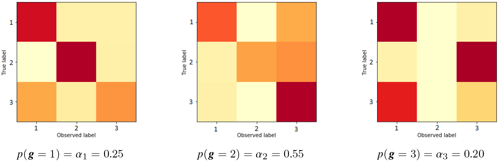
Verify groups on simulation
Confusion matrices used to perform Setup (1) simulation, i.e. real groups.
To perform the simulations we use different levels of noise (Table 2) and generate the confusion matrices (groups). On this setting, we perform a visual comparison of the different annotators behavior (matrices) presented on the simulation and the ones found by the proposed methods.
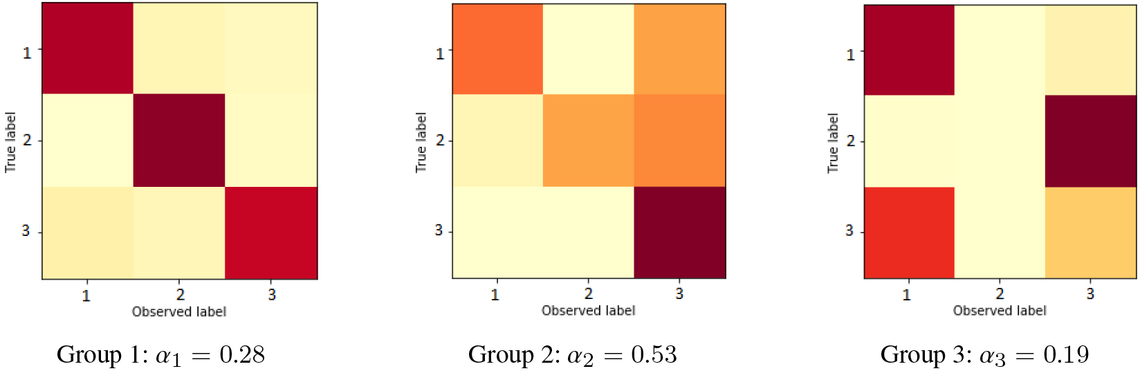
Confusion matrices found on Setup (1) with 100 by method CMM.
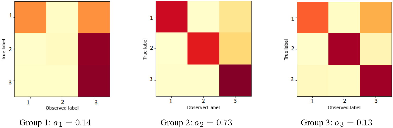
Confusion matrices found on Setup (1) with 100 by method C-MoA.
The generated confusion matrices or types of annotators on setup (1) are presented on Fig. 1, while for the groups found by the proposed methods (with 100) are shown in Figs 2 and 3. This illustrate how the C-MoA method is better than CMM to estimate the real simulated annotators type behavior (groups), being an ordered match between the simulated confusion matrices and the ones found by C-MoA. As the formulation of CMM method is to group annotations instead, the groups found by this method are different than the annotators types, as does not have the explicit information of the annotations origin. For example, first group, that has a bias for third class, capture a fraction of the behavior of the second and third simulated group. While the second and third group found by CMM, has the inexpert behavior of the first and second simulated annotator type. Similar results of comparison are observed on the different values and on the setup (2) simulation.
Groups analysis
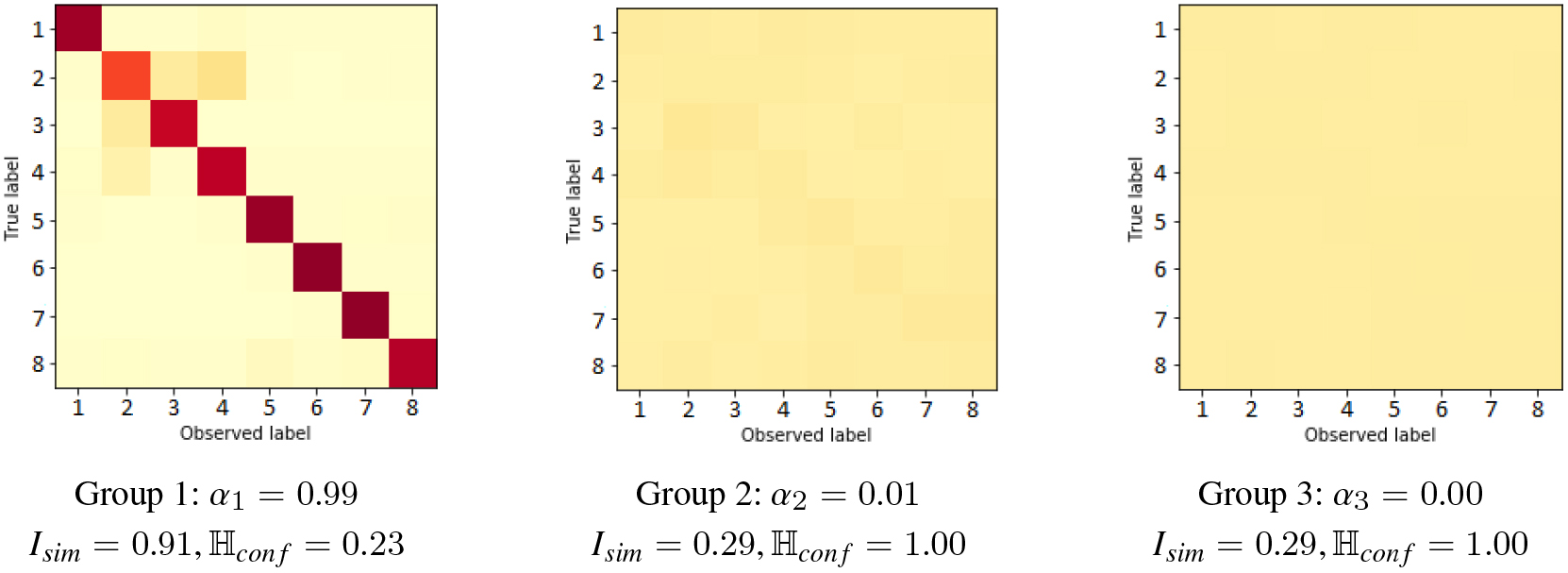
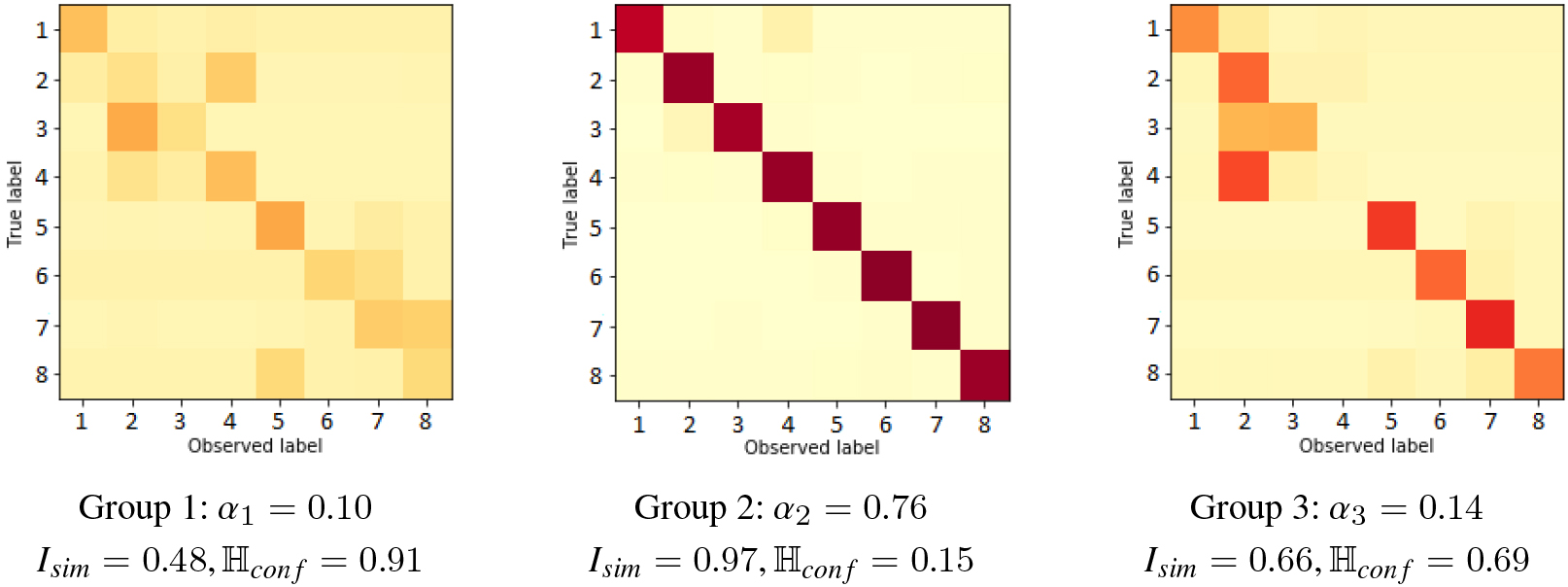
Confusion matrices found on LabelMe dataset by method CMM. Description metrics are shown below.
Confusion matrices found on LabelMe dataset by method C-MoA. Description metrics are shown below each group.
We visualize in Figs 4 and 5 the confusion matrices found by both proposed method on the LabelMe dataset. Also, below each matrix is shown the entropy of the confusion matrices (divided by to obtain a number in [0, 1]), their similarity with respect to the identity matrix (computed as 1 minus the normalized JS divergence, to obtain a number in [0, 1]) and the value of the mixing coefficients (prevalence of each group). We conclude that the CMM method found a group with a quite expert behavior (high , low ) and a presence of 99%, also a group of random spammers (maximum entropy) behavior with a prevalence of 1%. The third component has an insignificant presence in the mixture ( 0 rounding at two decimals) which shows that the method can easily adapt if the number of real groups in the data is lower than those specified into the model. While, the C-MoA method found quite different annotators groups: first component has quite inexpert behavior (low and high ), second shows an expert structure ( close to 1), and third is between these two, with a slight bias for the second class. A connection between the methods is that the behavior of first group on CMM is similar to a mixture of the second and third annotator group of C-MoA. Now, regarding the error patterns of the labeling process, it can be seen how are some confusions that trigger annotators to label with the second class (inside city landscape).11
Third and fourth class of LabelMe dataset are tall building and street, so they are regular or possible mistakes to found on the learning from crowds problem.
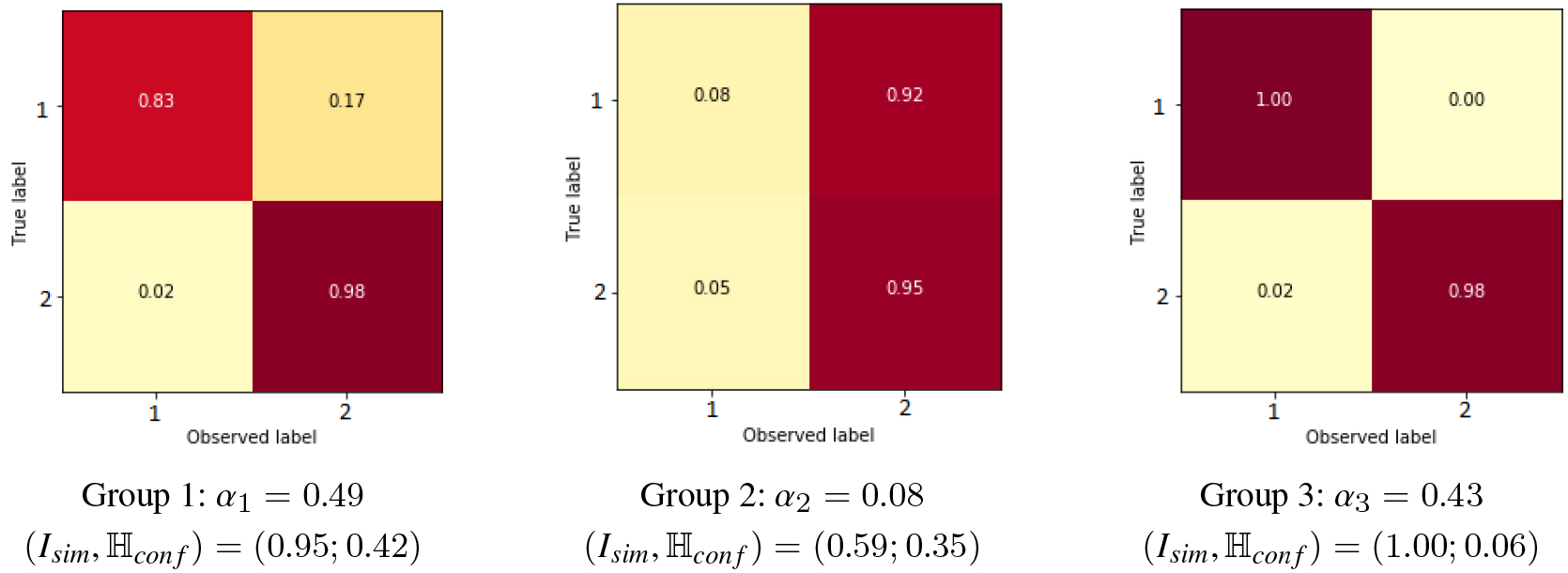
Confusion matrices found on Sentiment dataset by method CMM. Description metrics are shown below.
Confusion matrices found on Sentiment dataset by method C-MoA. Description metrics are shown below.
The same analysis is presented on the Sentiment dataset in Figs 6 and 7. The CMM method found a perfect behavior on the first component (identity matrix), equally to the third group of C-MoA, with 1, and also similar to the first, with slightly higher. This shows that are some cases when the annotators actually detects the ground truth. While, the second and third component of CMM express inexpert behavior with similar metrics () but in a complementary way, having a bias (or error pattern) for first (negative) and second (positive) class respectively. Also, the second component of C-MoA has a biased spammer behavior over the second class, perhaps exemplifying the trend of some annotators to labeling a text as positive.
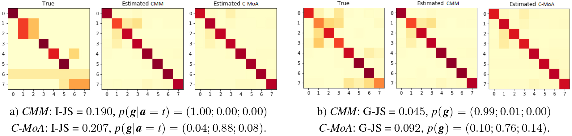
The confusion matrices found by the methods on both real datasets shows that different solutions could be obtained with good results. This mean that could be more than one unique way to find the different behaviors into the components that allow to solve the learning from crowd problem. Finally, Fig. 8 presents visual examples of the predictions of the confusion matrix corresponding to individual annotators and the global confusion matrix (Individual and Global settings) by both proposed methods. Here it can be seen how all confusion matrices are used by the probability assignment to build the predictions of every annotator .
Examples of individual (a) and global (b) confusion matrices estimation (True vs Estimated) by both proposed methods on LabelMe dataset. The individual matrix correspond to a random annotator .
Scalability comparison
Comparison of execution time per iteration by increasing on simulated data Setup (1).
In Fig. 9, we compare the execution time of proposed methods and baselines in the simulated setup (1) scenario. In contrast to proposed method and MV, the computational complexity of DL-EM increases monotonically with the value of . The aggregation phase realized by MV is the experimental lower bound of time due its simplicity. The gap between proposed methods shows that C-MoA is more expensive. This is because it depends on all the individual annotations and also it need to train an additional model of group assignment, contrasting to the vector parameters modeled by CMM. Indeed, this method has practically the same temporal complexity of train the DL model, so that any other aggregation method that use the DL model will have similar time or higher than CMM.
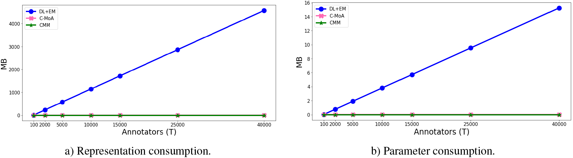
Comparison of memory consumption (in MB) by increasing on simulated data Setup (2). The DL-DS method is not shown because is practically the same as DL-EM method.
In Fig. 10, we compare the memory consumption of proposed methods and DL-EM in the simulated setup (2) scenario.12
MV method is not shown as it does not have parameters and representation is the same as CMM.
The representation consumption (a) that gather all the inputs to the models and the parameter consumption (b) that gather values in Table 1 (excluding DL parameters ), show similar behavior expressed in Fig. 9. It can be seen how both proposed method have a much lower and constant consumption than the baseline DL-EM. The baselines usually will increase the parameters with the number of annotators , as DL-EM and DL-DS use a confusion annotator per annotator (), others more complex method use a learning model per annotator (), with .
The scale of both Figs 9 and 10 shows that the greater consume comes from the data representation. This express that the consumption weakness of the baselines come from the denseassumption setting. All these results shows that both methods, specially CMM, could computational scale better to large scenarios on execution time and memory consumption as expected from its formulation, being practically constant to variation on the value.
Conclusion
We presented two models for learning from crowds that simplify previous existing methods. The main difference is that we do not represent annotators separately but model a fixed number of components into which the annotations and annotator behavior can be grouped together. The two models are proposed on different setting scenarios, the C-MoA method is based on the individual representation of the data, grouping annotator behavior. The CMM method is based on the global representation of the data, grouping annotation behavior. The different behaviors on the annotation process is modeled through a confusion matrix, as previous results suggest. Our results show that these models achieve competitive accuracy in scenarios with several labels per annotator, but can outperform the baselines when the distribution of labels is sparse by keeping the good results on the confusion matrix estimation. Another advantage is that the methods are more scalable (memory consumption and execution time) than other approaches in cases with large number of annotators, being practically constant on that factor. In accuracy performance, the C-MoA is the best option for small-medium scenarios or dense labels setting, while CMM is the best option for large scenario or sparse labels setting. In the scalability, the CMM is the lighter and faster proposed method into the learning from crowd problem. In future work, we plant to adapt our method in order to avoid the use of the EM algorithm.
Footnotes
Acknowledgments
Francisco Mena thanks the Programa de Iniciación Científica PIIC-DGIP of the Federico Santa María University for funding this work.
References
1.
SnowR.O’ConnorB.J.D. and NgA.Y., Cheap and fast – but is it good: evaluating non-expert annotations for natural language tasks, in: Proceedings of Conference on Empirical Methods in Natural Language Processing, 2008, pp. 254–263.
2.
ZhengY.LiG.LiY.ShanC. and ChengR., Truth inference in crowdsourcing: Is the problem solved, Proceedings of the VLDB Endowment10(5) (2017), 541–552.
3.
ZhangJ.WuX. and ShengV.S., Imbalanced multiple noisy labeling, IEEE Transactions on Knowledge and Data Engineering27(2) (2015), 489–503.
4.
DawidA.P. and SkeneA.M., Maximum likelihood estimation of observer error-rates using the EM algorithm, JSTOR: Series C (Applied Statistics)28(1) (1979), 20–28.
5.
ZhangY.ChenX.ZhouD. and JordanM.I., Spectral methods meet EM: A provably optimal algorithm for crowdsourcing, JMLR17(1) (2016), 3537–3580.
6.
SinhaV.B.RaoS. and BalasubramanianV.N., Fast Dawid-Skene: A Fast Vote Aggregation Scheme for Sentiment Classification, arXiv preprint arXiv:1803.02781, 2018.
7.
RaykarV.C.YuS.ZhaoL.H.ValadezG.H.FlorinC.BogoniL. and MoyL., Learning from crowds, Journal of Machine Learning Research11 (2010), 1297–1322.
8.
KajinoH.TsuboiY. and KashimaH., A Convex Formulation For Learning From Crowds, Trans. of the Japanese Society for Artificial Intelligence27 (2012), 133–142.
9.
AlbarqouniS.BaurC.AchillesF.BelagiannisV.DemirciS. and NavabN., Aggnet: Deep learning from crowds for mitosis detection in breast cancer histology images, IEEE Transactions on Medical Imaging35(5) (2016), 1313–1321.
10.
RodriguesF. and PereiraF.C., Deep Learning from Crowds, in: The Thirty-Second AAAI Conference on Artificial Intelligence (AAAI), 2018, 2018.
11.
MenaF. and ÑanculefR., Revisiting Machine Learning from Crowds a Mixture Model for Grouping Annotations, in: Iberoamerican Congress on Pattern Recognition, Springer, 2019, pp. 493–503.
12.
McLachlanG. and BasfordK.E., Mixture Models, Marcel Dekker Inc., 1987.
13.
McLachlanG. and KrishnanT., The EM algorithm and extensions, Vol. 382, John Wiley & Sons, 2007.
14.
DempsterA.P.LairdN.M. and RubinD.B., Maximum likelihood from incomplete data via the EM algorithm, JSTOR: Series B39(1) (1977), 1–22.
15.
ShengV.S.ProvostF. and IpeirotisP.G., Get another label? improving data quality and data mining using multiple, noisy labelers, in: Proceedings of the 14th ACM SIGKDD, ACM, 2008, pp. 614–622.
16.
RodriguesF.PereiraF. and R.B., Learning from multiple annotators: distinguishing good from random labelers, Pattern Recognition Letters34 (2013), 1428–1436.
17.
SmythP.FayyadU.M.BurlM.C.PeronaP. and BaldiP., Inferring ground truth from subjective labelling of venus images, in: NIPS, 1995, pp. 1085–1092.
18.
WhitehillJ.WuT.-f.BergsmaJ.MovellanJ.R. and RuvoloP.L., Whose vote should count more: Optimal integration of labels from labelers of unknown expertise, in: NIPS, 2009, pp. 2035–2043.
19.
ZhouD.BasuS.MaoY. and PlattJ.C., Learning from the wisdom of crowds by minimax entropy, in: Advances in Neural Information Processing Systems, 2012, pp. 2195–2203.
20.
YanY.RosalesR.FungG.SchmidtM.HermosilloG.BogoniL.MoyL. and DyJ., Modeling annotator expertise: Learning when everybody knows a bit of something, in: Proceedings of the XXX AISTATS, 2010, pp. 932–939.
21.
BiW.WangL.KwokJ.T. and TuZ., Learning to Predict from Crowdsourced Data., in: UAI, 2014, pp. 82–91.
22.
GuanM.Y.GulshanV.DaiA.M. and HintonG.E., Who said what: Modeling individual labelers improves classification, in: Thirty-Second AAAI Conference on Artificial Intelligence, 2018.
23.
LiuY.ZhangW.YuY. et al., Truth inference with a deep clustering-based aggregation model, IEEE Access8 (2020), 16662–16675.
24.
DiasJ.G. and WedelM., An empirical comparison of EM, SEM and MCMC performance for problematic Gaussian mixture likelihoods, Statistics and Computing14(4) (2004), 323–332.
25.
AbbiR.El-DarziE.VasilakisC. and MillardP., Analysis of stopping criteria for the EM algorithm in the context of patient grouping according to length of stay, in: 2008 4th International IEEE Conference Intelligent Systems, Vol. 1, IEEE, 2008, pp. 3–9.