Interpretable and effective hashing via Bernoulli variational auto-encoders

Abstract

Due to the rapid increase in the amount of data generated in many fields of science and engineering, information retrieval methods tailored to large-scale datasets have become increasingly important in the last years. Semantic hashing is an emerging technique for this purpose that works on the idea of representing complex data objects, like images and text, using similarity-preserving binary codes that are then used for indexing and search.

In this paper, we investigate a hashing algorithm that uses a deep variational auto-encoder to learn and predict the codes. Unlike previous approaches of this type, that learn a continuous (Gaussian) representation and then project the embedding to obtain hash codes, our method employs Bernoulli latent variables in both the training and the prediction stage. Constraining the model to use a binary encoding allow us to obtain a more interpretable representation for hashing: each factor in the generative model represents a bit that should help to reconstruct and thus identify the input pattern. Interestingly, we found that the binary constraint does not lead to a loss but an increase of search accuracy. We argue that continuous formulations learn a representation that can significantly differ from the code used for search. Minding this gap in the design of the auto-encoder can translate into more accurate retrieval results. Extensive experiments on seven datasets involving image data and text data illustrate these findings and demonstrate the advantages of our approach.

Keywords

Hashing variational autoencoders deep learning Gumbel-Softmax distribution neural information retrieval

1. Introduction

Many applications in computer science are based on similarity search, i.e., finding elements in a database that are similar to a given sample object [1]. The greater availability of complex data types such as image, audio, and text, has increased the interest for this type of search in the last years and raised the need for methods that can reduce the processing time and storage cost of traditional paradigms. Tree-based indexing methods such as KD-trees, Ball-trees and R-trees have been shown to degrade quickly as the dimensionality of the data (descriptors) increases [46], and thus novel approaches, often tailored to large-scale image retrieval, have started to be investigated. Among these techniques, hashing algorithms have received significant attention.

The purpose of hashing techniques is to represent the data using compact binary codes that preserve their semantic content and can be used as cells into a hash table. Items similar to a query can then be found by accessing all the cells of the table that differ a few bits from the query. As binary codes are storage-efficient, hashing can be performed efficiently in main memory even for very large datasets [34].

Hashing algorithms can be broadly categorized into data-independent and data-dependent methods. Data-independent methods exploit properties of some probability distributions to ensure that the similarity function of the original space is approximately preserved by the embedding into the code space [22]. These methods usually require codes much longer than those obtained with data-dependent techniques, that leverage data and machine learning techniques to explicitly optimize the embedding, at the cost of some training time [38, 50]. Supervised, unsupervised and semi-supervised approaches have been studied. Supervised methods rely on explicit annotations, such as topic or similarity labels, to learn the hash codes. For instance, [24] implements a hash function by training a deep neural net on pairs of images previously labelled as similar or dissimilar examples. Unfortunately, the performance of these methods degrades quickly when there is not enough labelled data for training or it is noisy. Unsupervised methods deal with this issue, providing learning mechanisms that do not require explicit supervisory signals [38] and can thus leverage unlabelled data, which is usually abundant and cheap [45]. Often, these methods can be transformed into semi-supervised models that can also exploit labels if available.

Recently, significant progress has been made in the field of deep generative models. The so-called variational autoencoder (VAE) framework [19], provides algorithms for probabilistic inference and learning that scale to very large datasets and provide state-of-the-art performance in many tasks. A natural question is whether these advances can be exploited to devise novel hashing algorithms. It has been shown indeed that VAEs can be successfully trained to learn hash codes [5], improving on previous techniques when labelled data is scarce. A disadvantage of this approach is that, as conventional VAEs use a Gaussian encoder, the continuous representation learnt by the model needs to be quantized to obtain binary codes. This step introduces an error that is not account for in the learning process and can seriously degrade information retrieval performance. Also, it is difficult to interpret this model as a hash function, because there is nothing that rewards learning binary codes in the training phase.

In this paper, we propose to learn a deep hashing model using a VAE with Bernoulli latent variables that maps an object or input pattern directly to a binary code representation of the different bits. The main technical difficulty of this approach, i.e. back-propagation through discrete nodes, can be circumvent by specializing the method proposed in [17] to handle Bernoulli distributions [30]. Experiments on text and image retrieval tasks demonstrate that this approach works well for unsupervised hashing, leading to more effective and interpretable binary codes than those produced by a continuous VAE and state of the art methods.

This work is an extension of the research presented in [32]. The main differences are:

•
Related work has been extended.
•
The experiments are expanded by adding 3 image domain datasets and 1 text domain dataset, using Deep Learning models.
•
The discussion and analysis regarding the quantization factor of the learned representation is extended.

The rest of this paper is organized as follows. In the next section, we outline the idea of hashing for similarity search. Related work is discussed in Section 3. In Section 4, we present the proposed formulation. In Section 5, we report experimental results, comparing the codes of our method with those of a continuous VAE. Finally, Section 6 summarizes the conclusions and final remarks of this work.
2. Problem statement and background

2.1 Similarity search

Consider a dataset $D=\{x^{(1)},x^{(2)},\ldots,x^{(n)}\}$ , with $x^{(\ell)}\in\mathbb{X}\ \forall\ell\in[n]=\{1,\ldots,n\}$ , and the problem of searching $D$ to find elements that are similar to some sample object $q\in\mathbb{X}$ (not necessarily in $D$ ) referred to as query. If $\mathbb{X}$ is equipped with a similarity function $s:\mathbb{X}\times\mathbb{X}\to\mathbb{R}$ , such that the greater the value of $s$ , the more similar are the objects, and $n$ is small, a simple approach to solve this problem is a linear scan: compare $q$ with all the elements in $D$ and return $x^{(\ell)}$ if $s(x^{(\ell)},q)$ is greater than some threshold $\theta$ . The value of $\theta$ (search radius), can be given in advance, computed to return exactly $k$ results or chosen to maximize information retrieval metrics such as precision and recall [1]. If $\mathbb{X}\subset\mathbb{R}^{d}$ , with small $d$ , specialized data structures (e.g. KD-trees) perform efficient scans when $n$ is large. Unfortunately, if $d$ becomes large, as in large-scale collections of images, audio, and text, the performance of these data structures degrades quickly [34] and novel methods are required.

2.2 Hashing

Hashing algorithms address similarity-search problems by devising an embedding $h(\bm{x})$ of the feature space $\mathbb{X}$ into the Hamming space $\mathbb{H}_{B}=\{0,1\}^{B}$ , and substituting searches in $\mathbb{X}$ by searches in $\mathbb{H}_{B}$ . Since binary codes can be efficiently stored and compared, searches in $\mathbb{H}_{B}$ can be orders of magnitude faster, even using a simple $\mathcal{O}(n)$ linear scan. The common goal of the hashing approaches is that the embedding has to preserve similarity on the semantic content of the objects.

2.3 Quantization error

Many hashing approaches obtain $h(\bm{x})$ by learning a continuous embedding $\phi(\bm{x})\in\mathbb{R}^{B}$ that is then discretized by thresholding, i.e. by computing $h(\bm{x})=\bm{1}(\phi(\bm{x})-b)$ , where $\bm{1}(\cdot)$ denotes the indicator function. The term $\|h(\bm{x})-\phi(\bm{x})\|$ is called the quantization error and can have a significant impact in the quality of the obtained hashes for search applications [11], besides it depend of an external manual-defined bias $b$ .

2.4 Focus

We focus on learning a hash function $h(\cdot)$ using a deep probabilistic graphical model that reduces the quantization error. Our final goal is to obtain better codes for similarity search tasks focused on the unsupervised case, but semi-supervised extensions in the vein of [5] are not hard to obtain. Our validation is performed on text and image domain datasets.

2.5 Standard loss functions on discrete data

Many machine learning approaches used information functions as loss function or quality measurements. For example, consider a categorical random variable $X\in\mathbb{X}$ with probability distribution $p_{x}=p(X=x)$ . In a Bernoulli random variable case ( $X\in\{0,1\}$ ) we will have only one probability $p=p(X=1)=1-p(X=0)$ . Based on this, the entropy of the probability distribution $p$ is given by

$\displaystyle H(p)=-\sum_{x\in\mathbb{X}}p_{x}\log{p_{x}}\quad\text{binary}:H(% p)=-p\log{p}-(1-p)\log{(1-p)}\ .$ (1)

The cross entropy of another probability distribution $q$ (defined in the same way for $p$ over other discrete random variable $Z\in\mathbb{X}$ ) relative to the probability distribution $p$ is given by

$\displaystyle H(p,q)=-\sum_{x\in\mathbb{X}}p_{x}\log{q_{x}}\quad\text{binary}:% H(p,q)=-p\log{q}-(1-p)\log{(1-q)}\ .$ (2)

The Kullback-Leibler divergence (or KL divergence) from $q$ to $p$ is given by:

$\displaystyle D_{\text{KL}}(p||q)=\sum_{x\in\mathbb{X}}p_{x}\log{\frac{p_{x}}{% q_{x}}}\quad\text{binary}:D_{\text{KL}}(p||q)=p\log{\frac{p}{q}}+(1-p)\log{% \left(\frac{1-p}{1-q}\right)}$ (3)

The mathematical relation between these concepts (entropy, cross entropy and KL divergence) is given by: $H(p,q)=H(p)+D_{\text{KL}}(p||q)$ .

3. Related work

The problem of representing data using binary codes that preserve semantic content and support efficient indexing has been extensively studied in the last years. Below we present a brief description of the main ideas developed in the literature, stressing the relationships and differences between our approach and previous research.

3.1 Randomized methods

Early hashing algorithms were randomized methods devised to preserve specific similarity functions or distance metrics [3, 15]. For instance, SimHash [6], based on random projections, was devised to approximately preserve cosine similarity, a function widely used to compare documents in the vector space model (VSM). MinHash [40, 3] preserves the “resemblance” or Jaccard similarity of two documents by using random permutations of sets (bags of words). E2LSH [7] was created to approximately preserve the Euclidean distance used e.g. in image search applications.

All these and more data-independent approaches to hashing can be described as particular cases of the so-called Locality Sensitive Hashing (LSH, [7]) framework. Unfortunately, despite the strong theoretical guarantees that the framework provides in the limit of many bits [10], the performance of these techniques is often unsatisfactory in applications that require compact hash keys (low memory footprint) or in scenarios where search needs cannot be easily encoded into a similarity function. Learning based methods, such as that proposed in this paper, attempt to overcome these limitations using machine learning formulations to optimize the hash codes.

3.2 Shallow learning based approaches

As real data often lie in a low-dimensional sub-space (or manifold) of the feature space [18], data-dependent methods can dramatically reduce the number of bits required to preserve similarity by learning and projecting the data into a set of directions that summarize the data distribution. If available, learning based methods can also exploit annotations to surrogate the knowledge of a specific similarity function.

AnnoSearch [49], one of the first data-dependent approaches to hashing, computes the bits by projecting the data into the top PCA directions, i.e. the best fitting sub-space in terms of variance preservation. SSH [44] relaxes the orthogonality constraints of this method to obtain more balanced projections (and so bits) in terms of explained variance. KLSH [22] uses kernel methods to implicitly perform PCA in a high-dimensional feature space where linear relationships can be more easily found. ITQ [11] improves PCA based hashing by learning a rotation matrix that minimizes the quantization error introduced by a continuous formulation of hashing.

In a different and influential vein, Spectral Hashing (SpH) [50] poses hashing as the problem of partitioning a similarity graph, where the vertices represent training points and the edges are weighted using similarity scores that are computed using a kernel. Each bit of the codeword identifies a (different) partition of the graph that should have as low cut as possible to optimize the intra-cluster (within) similarity of the groups. As pointed out in [28], the extension of SpH to unseen data is based on strong assumptions about the data distribution that ignores the information provided by the training data. Anchor Graph Hashing (AGH) attempts to overcome this limitation using the Nystrom method on a sub-graph of the original similarity graph that approximates its geometric structure. As both SpH and AGH determine the hash bits by thresholding eigenfunctions of a similarity graph Laplacian, these approaches relate hashing to manifold learning techniques for dimensionality reduction that have emerged in the last years [48, 18]. Unfortunately these techniques are often very sensitive to the choice of the metric used to build the neighbourhood graph.

In contrast to spectral and PCA-based methods, our method is an unsupervised approach [12] that learns the data distribution without the assumption of a specific similarity function or kernel. Supervised hashing algorithms such as LDA-Hash [43], CCA-ITQ [11], BRE [21] and SSH [45] succeed in this goal, but assumes that some type of metadata which conveys information about the data similarity structure is available. For instance, CCA-ITQ extends ITQ using pointwise annotations, e.g. topic or category labels. LDA-Hash [43] improves the projection directions of PCA-based hashing assuming that pairwise annotations (similar/dissimilar pairs) are available. In the same vein, KLSH [27] and MLH [33] learn more discriminative directions by explicitly penalizing the distances between similar points. Even more complex supervision schemes, such as triplets of examples has been explored [47, 54], and hence, there is plenty of methods we can use assuming supervision. Unfortunately, annotation procedures are often expensive and slow to be adopted in many applied domains. On the other hand, with budgeted data, these methods are prone to over-fitting, leading to unsatisfactory search performance.

3.3 Deep learning methods

Deep learning methods typically improve hashing by learning a representation of the input data that works well for the task [12], that is, they equip the model with a learnable transformation $g:\mathbb{X}\to\mathbb{Z}$ from the original input space $\mathbb{X}$ to a new feature space $\mathbb{Z}$ on which the hash function $h:\mathbb{Z}\to\{0,1\}^{B}$ is finally learned. For instance, the method in [29, 24] learns the map $g:X\to Z$ using a feed-forward neural net [12] and obtains the hash codes $h$ by simply thresholding the (continuous) representation learned by the net $z=g(x)$ . The unsupervised variant of the method, termed Deep Hashing (DH), overcomes the linearity shortcoming of PCA-based hashing [49, 11], but adopts essentially the same objective: to maximize the variance of the embedded data. Relaxed orthogonality constraints are applied to the weights matrices of all the layers and a term assessing the quantization loss is introduced into the training objective. In the supervised variant (SDH), the model is trained to minimize the intra-class variations and maximize the inter-class variations, as in many previous hashing approaches (e.g. LDA-Hash [43]). Treating the hash bits as fixed after the forward pass circumvents the need of mixed discrete-continuous optimization solvers and allows to train the models using back-propagation [29].

Departing from previous image retrieval applications based on hand-crafted descriptors such as GIST or SIFT, Deep Supervised Hashing (DSH) [26] uses a convolutional neural net (CNN, see [36] for a review) to extract those features directly from images. The difficulty of learning visual features and hash codes simultaneously is circumvented using a two-stage approach originally proposed in [23]. The first stage learns hash codes for the training examples using a formulation closely related to KLSH [27]. The second stage trains a supervised model to reproduce the codes learned in the first stage. By decomposing the task in this way, specialized solvers are required only for the first stage and the neural net can be trained using standard back-propagation. The same strategy is employed in [51], where one-dimensional CNNs are trained for text hashing. In this case however, the hash codes of the first stage are obtained using a supervised variant of Spectral Hashing (SpH) [50] and pre-trained word embeddings (GloVe) are used to feed the text into the net.

Our review of recent research confirms this tendency to construct deep hash functions using pre-trained models also in image retrieval. For instance, the method in [52] uses the first $6-7$ layers of VGGNet[42] or AlexNet[20] to obtain convolutional features that are then fine-tunned (specialized) for hashing using a supervised objective. The method in [39] uses the first $7$ layers of VGGNet even without fine-tunning, i.e. as non-trainable feature detectors, and learns a linear hash function to map that representation to the Hamming space. The method in [39] uses the entire VGGNet model for hashing, modifying the number of neurons in the output layer according to the code length and activating them with a hyperbolic tangent (tanH) function. The model can be fined-tuned for hashing thanks the approach in [23]: hash codes are first obtained for a training set using a variant of Spectral Hashing [50], and a net is then trained to perform out-of-sample predictions. After training is complete, binary codes are obtained by passing the output layer through a sign function, i.e. projecting the output activations into the two saturating points of the non-linearity ( $\pm 1$ ). A novel aspect of this approach w.r.t. previous deep learning methods resorting on [23] is that the problems of graph partitioning and network training are iterated. At each iteration, intermediate layers of the CNN are used to update the similarity graph employed by the first stage and thus the target of the second stage.

3.4 Autoencoders

As autoencoders play a fundamental role in unsupervised learning [2], our method is naturally related to hashing techniques that exploit this machinery to circumvent the need of explicit annotations. As in other deep learning approaches, these methods learn an encoding function $g_{e}:\mathbb{X}\to\mathbb{Z}$ , from the input space $\mathbb{X}$ to a feature space $\mathbb{Z}$ , and obtain the hash function by projecting $z=g_{e}(x)$ onto the binary space. The key difference w.r.t. other deep learning approaches is that $z$ is optimized such that it is possible to reconstruct $x$ from $z$ using a decoding function $g_{d}:\mathbb{Z}\to\mathbb{X}$ . Traditional autoencoders employ a deterministic encoder $g_{e}$ and decoder $g_{d}$ .

In [4], a linear autoencoder is used to learn hash codes. The model, termed Binary Autoencoder (BA), is trained to minimize the reconstruction error $\|x-g_{d}(g_{e}(x))\|_{\ell_{2}}^{2}$ with an explicit binary constraint on the transformation learned by the encoder: $g_{e}(x)\in\{0,1\}^{B}$ . Due to this constraint, the model cannot be trained with standard back-propagation methods and a mixed integer programming solver, involving a nested optimization loop, needs to be applied. The method in [8], termed UH-BDNN, employs an asymmetric autoencoder architecture: a linear function is used for the decoder $g_{d}$ but a deep feed-forward net is used to implement the encoder $g_{e}$ . As in [4], binary representations are enforced using explicit constraints that have to be handled with a specialized solver which alternates two optimization steps. In spite of their computational complexity, experiments in [4, 8] are encouraging and suggest that hashing based on autoencoders can be more effective in unsupervised scenarios than other shallow and deep learning methods such as DH [24, 29].

Tailored to large-scale image retrieval, the method in [9] replaces the feed-forward layers used in previous research by convolutional layers, which can learn more easily the local patterns that often arise in image data. In contrast to the work of [4], this method introduces the binary constraints as penalties into the objective function, which allows the model to be trained with gradient descent. The method uses also regularization terms present in various previous formulations (e.g. [11]) that maximize the variance of the learned representation and enforce the bits to be pairwise uncorrelated.

3.5 Deep graphical models

In practice, the variational autoencoder (VAE) we propose in this paper has an architecture similar to the traditional autoencoders described in Section 3.4. However, as we cast the problem of learning the representation $z$ as an inference problem, our encoder does not learn a deterministic transformation $z=g_{e}(x)$ but a stochastic map $q_{\phi}(z|x)$ . Thereby, these models learn the most likely region where the input pattern should be, unlike deterministic autoencoders that learn the specific most likely point. In our method, neural nets are not directly used to implement the encoder or decoder, but to parametrize the distributions involved in the generating process. An advantage of this approach is that we can easily incorporate prior knowledge about the desired representation $z$ , enforcing a prior distribution on the latent space. We can also select the form of the posterior $q_{\phi}(z|x)$ to introduce an inductive bias that helps the learner to find feasible and meaningful solutions. In addition, representing hashing through a probabilistic graphical model facilitates the interpretation of the results by humans, which is a topic of emerging importance nowadays.

Up to our knowledge, the use of a graphical model to learn hash codes without supervision was first proposed in [38] with the so-called Semantic Hashing (SH) approach. The model was composed of multiple layers of latent variables. The top two layers formed a Restricted Boltzmann Machine (RBM) and the remaining layers defined a Deep Belief Net (DBN) with directed top-down connections. At the training stage, the activation of the binary nodes in the deepest layer allowed to identify topics from which the visible nodes had to reconstruct the input data, just as an autoencoder does. Indeed, SH can be seen today as a stochastic autoencoder where encoder and decoder share architecture and weights. Unfortunately, training this model is often computationally hard because it is based on layer-wise pre-training and specialized optimization routines. Perhaps for this reason, most subsequent research on unsupervised hashing preferred shallow architectures or replaced the graphical model by a traditional autoencoder (Section 3.4).

There are some exceptions to the latter. In [55], a graphical model for multi-modal hashing is presented. The method adopts a maximum a-posteriori (MAP) formulation that requires intra-modality and inter-modality labels. In addition, the method learns codes for the training set only, and complex out-of-sample extensions are required to hash novel data. In similar fashion, the method in [53] adopts MAP inference for learning and a linear extension for out-of-sample predictions. More recently, a complete probabilistic treatment of hashing, that avoids MAP inference, has been presented in [14]. Unfortunately, this algorithm requires pairwise annotations, relies on a continuous relaxation of the code distributions, and requires an out-of-sample extension to hash novel data. Finally, in the vein of [55] and [53], this method does not exploit deep learning to build the hash function.

3.5.1 Variational autoencoders

In the last years, significant progress has been made in the field of deep generative models. In particular, it has been shown that Variational Autoencoder (VAE) models [19] lead to efficient algorithms for topic modeling and text hashing [5, 41]. The method in [5] obtains hash codes by first training a standard VAE, i.e., a stochastic autoencoder with a Normal latent distribution, and then thresholding the learned representation around the median (zero). Setting the threshold at the median encodes the prior belief that, in a balanced hash table, half of the bits should be active and half inactive. This method, named Variational Deep Semantic Hashing (VDSH), improves the results of previous unsupervised techniques on text hashing, besides being more scalable and stable than the prior work of [38].

A discrete (categorical) VAE (Ca-VAE) for discovering topics in text documents is presented in [41]. The latent variables are modeled with a Multinomial distribution such that only one topic can be present at the same time on a document. Though useful in the context of text clustering, the latter constraint makes the technique difficult to adapt for hashing.

4. Proposed method

Motivated by the effectiveness of variational autoencoders [19] to learn latent representations, we pose hashing as an inference problem where the objective is to learn a posterior distribution $q_{\phi}(\bm{b}|\bm{x})$ of the code $\bm{b}\in\{0,1\}^{B}$ corresponding to an input pattern $\bm{x}$ . In this framework, we are thus assuming that the observed data $\bm{x}$ can be reconstructed by a random process involving two steps: (i) a hash code $\bm{b}$ is first generated according to some prior distribution $p_{\theta}(\bm{b})$ , and then (ii) a value $\bm{x}$ is generated according to a conditional distribution $p_{\theta}(\bm{x}|\bm{b})$ . This generative process can be thought of as choosing a “bucket” in a hash table of size $2^{B}$ and then sampling the observations contained in that bucket. We can learn $q_{\phi}(\bm{b}|\bm{x})$ in such a way that this random process approximates well the real distribution of the data. This is the core of our approach.

In the literature, the distribution $q_{\phi}(\bm{b}|\bm{x})$ is called the encoder, and the distribution $p_{\theta}(\bm{x}|\bm{b})$ the decoder or the generator. The main concern in this paper is learning a hash function $h:\mathbb{X}\to\mathbb{H}_{B}$ and thus the encoder $q_{\phi}(\bm{b}|\bm{x})$ . The generative process sketched above is an auxiliary task used to create a surrogate of the supervisor, that in the setting we address is not available. Most applications of the variational autoencoder (VAE) framework [19] in contrast, are focused on the generator, and use the decoder as an auxiliary distribution that can be discarded once learning has been done. In spite of being less common, this “inverse approach” has been successfully applied in recent works involving topic modelling [41] and hashing [5]. The key difference between our model and [5] is that we choose the random variable $\bm{b}$ , representing the code to be binary and, consequently, the distribution $q_{\phi}(\bm{b}|\bm{x})$ to be a multi-variate Bernoulli i.e. $\bm{b}\sim\text{Ber}(\alpha(\bm{x}))$ .

Resorting to a more standard formulation of the VAE, [5] chooses $q_{\phi}(\bm{b}|\bm{x})$ to be a Gaussian $\mathcal{N}(\mu(\bm{x}),\sigma(\bm{x}))$ and, consequently, $\bm{b}$ to be a continuous random variable. This choice has two main shortcomings. First, it is no clear why a continuous representation should serve well for binary indexing and search. The main advantage of Bernoulli formulation is thus interpretability. That means that $\forall i\in{1,\ldots,B}$ , the latent factor $b_{i}\in\{0,1\}$ can be understood as a bit of the hash code assigned to $\bm{x}$ . The generative process should be able to approximately reconstruct the input pattern from these bits, exactly as we expect of a similarity preserving hash table. If $\bm{b}$ is Gaussian in contrast, the relationship between the hash codes and the representation learnt by the model is more ambiguous. The generative process have been trained to reconstruct the observation from a continuous low dimensional representation that may be very different from its binary projection, that is then used for search. The second advantage of our formulation regards thus the smaller gap between the learned representation and binary code. The method in [5] uses indeed a simple thresholding operation on the Gaussian representation $\bm{z}_{g}$ once learning is complete: $\bm{b}=\bm{1}(\bm{z}_{g})$ , where $\bm{1}(\cdot)$ denotes the indicator function. This step can incur into a significant quantization error that seriously degrades the similarity search performance of the hash codes.

Figure 1.

1-bit quantization of a Gaussian variable (standard VAE) and two Gumbel-Softmax variables (B-VAE) at different temperatures. In practice, all the points below/greater than 0 are rounded to $0$ / $1$ to obtain binary codes. A Gumbel-Softmax distribution at low temperature reduces the quantization error inducing a saturation around 0/1.

An illustration of the latter issue is provided in Fig. 1 for a single bit. Here we can see that, even if the distribution is optimally centered, samples from a Gaussian can significantly differ from their projections on the two bit states 0 and $1$ , which are used to index and search. We can see also that the Gumbel distribution [31], designed to explicitly approximate discrete random variables, can do a better job by tuning the parameter termed temperature. Indeed, as we discuss below, in order to obtain a simple and efficient learning algorithm, the Gumbel distribution will be a key component of our model, called Bernoulli-VAE (B-VAE).

4.1 Parametrization by neural nets

As in the traditional VAE, where the parameters of the Gaussian posterior $\mathcal{N}(\mu(\bm{x}),\sigma(\bm{x}))$ are represented using neural networks, we learn the activation probabilities $\alpha(\bm{x})$ of our multi-variate Bernoulli distribution $\text{Ber}(\alpha(\bm{x}))$ using a deep non-linear function $f(\bm{x};\phi)$ . To be able to train this model, we will resort to the auxiliary generator $p_{\theta}(\bm{x}|\bm{b})$ involved in the inverse process of reconstructing the input pattern $\bm{x}$ from its binary code $\bm{b}$ . The exact family we choose $p_{\theta}(\bm{x}|\bm{b})$ from depends on the type of data, but just like with the encoder, its parameters can be learned using a deep neural net $g(\bm{b};\theta)$ .

Due the current benefits and flexibility of deep learning models, the choice of learning the model parameters by neural nets, allow us to adapt the architecture of $f(\bm{x};\phi)$ to solve different complex problems. In problems where data is represented by traditional feature vectors, we can implement $f(\cdot)$ and $g(\cdot)$ using simple feed forward (FF) nets. In problems in which data involves sequences or context is needed, we can implement $f(\cdot)$ and $g(\cdot)$ using a recurrent architecture (RNN, [25] for a survey). In problems involving images or, more generally, signals with local patterns of variation, we can implement $f(\cdot)$ and $g(\cdot)$ using a convolutional net (CNN, [36] for a survey). Even so, $f(\cdot)$ could be a FF model and $g(\cdot)$ a CNN model. This imply that our framework is independent of the type of function used to process data and the idea can be used in many different applications. For this reason, we next refer to the trainable parameters of $f(\cdot)$ and $g(\cdot)$ as $\phi$ and $\theta$ , in the most general way possible.

4.2 Learning approach

The composition of the encoder $p_{\theta}(\bm{x}|\bm{b})$ and the decoder $q_{\phi}(\bm{b}|\bm{x})$ leads to a deep (stochastic) auto-encoder (VAE). The parameters $\phi$ and $\theta$ of this model can be learned by maximizing the data log-likelihood $\ell(\theta,\phi;D)$ . Unfortunately, since $\bm{b}$ is unobserved, optimizing $\ell$ is difficult. However, as proposed by [19], VAEs can be trained to maximize the theoretical lower bound of $\ell(\theta,\phi;D)$ . For a specific point $\bm{x}^{(\ell)}$ in $D$ , we can obtain the following lower bound:

$\displaystyle\ell(\theta,\phi;\bm{x}^{(\ell)})\geqslant\mathcal{L}=\mathbb{E}_% {q_{\phi}(\bm{b}|\bm{x}^{(\ell)})}\left[\log{p_{\theta}(\bm{x}^{(\ell)},\bm{b}% )}-\log{q_{\phi}(\bm{b}|\bm{x}^{(\ell)})}\right]\mathcal{L}=\mathbb{E}_{q_{% \phi}(\bm{b}|\bm{x}^{(\ell)})}\left[\log{p_{\theta}(\bm{x}^{(\ell)}|\bm{b})}% \right]-D_{\text{KL}}\left(q_{\phi}(\bm{b}|\bm{x}^{(\ell)})||p_{\theta}(\bm{b}% )\right)\,,$ (4)

where the first term of $\mathcal{L}$ corresponds to the expected success in the reconstruction of $\bm{x}$ from $\bm{b}$ , and the second measures the KL divergence between the posterior implemented by the encoder $q_{\phi}(\bm{b}|\bm{x})$ and some prior $p_{\theta}(\bm{b})$ manually defined. For common choices of $p_{\theta}(\bm{b})$ , the KL divergence can be integrated analytically, which leads to expressions easy to differentiate. However, traditional (Monte-Carlo) estimators of the first term in Eq. (4), lead to unstable gradients [19]. The framework presented in [19] solves this problem using the so-called re-parametrization trick. Unfortunately, this method does not apply for discrete latent variables and so we need a more specialized and recent method.

4.3 Re-parameterization via Gumbel-Softmax

As shown in [30], with the introduction of the CONCRETE distribution, and in [17], with the introduction of the Gumbel-Softmax distribution, samples of a discrete random variable can be well approximated by sampling a carefully designed continuous distribution. This idea can be adapted to the special case of Bernoulli random variables, as proposed in [30]. Indeed if $\bm{b}_{i,\ell}\sim q_{\phi}(\bm{b}_{i,\ell}|\bm{x}^{(\ell)})=\text{Ber}(% \alpha_{i}(\bm{x}^{(\ell)}))$ , $\bm{\epsilon}_{i}\sim\mathcal{U}(0,1)\,\forall i\in[B]$ , with $\sigma(\xi)=1/\left(1+\exp(-\xi)\right)$ the sigmoid or logistic function, we have that

$\displaystyle\hat{\bm{b}}_{i,\ell}=\sigma\left(\left(\log{\frac{\alpha_{i}(\bm% {x}^{(\ell)})}{1-\alpha_{i}(\bm{x}^{(\ell)})}}+\log{\frac{\bm{\epsilon}_{i}}{1% -\bm{\epsilon}_{i}}}\right)/\lambda\right)\,,$ (5)

converges to $\bm{b}_{i,\ell}$ in the sense that $P(\lim_{\lambda\to 0}\hat{\bm{b}}_{i,\ell}=1)=\alpha_{i}(\bm{x})$ . Thus, we can take samples of $\hat{\bm{b}}_{i,\ell}$ to obtain approximate samples of $\bm{b}_{i,\ell}$ . As depicted in Fig. 1, at low temperatures $\lambda$ , the probability of getting samples which are not 0 or 1 is very small, because Eq. (5) saturates at the extremes. Since, in addition, $\hat{\bm{b}}_{i,\ell}$ is a deterministic transformation of the auxiliary multivariate uniform random variable $\bm{\epsilon}$ , that does not depend on the encoder parameters $\phi$ , we can estimate $\mathbb{E}_{q_{\phi}(\bm{b}|\bm{x})}\left[\log{p_{\theta}(\bm{x}|\bm{b})}\right]$ by sampling several values on $p(\bm{\epsilon})$ . This leads to stable gradients in terms of the model parameters ( $\phi,\theta$ ), and then back-propagation can be used to train our VAE. As shown by [19], sampling only one value of the auxiliary noise is enough to correctly train the model. As recently pointed out by [35], the discrete sampling is mathematically difficult, so a good value of $\lambda$ should remain low during training. According to [17, 30] an annealing process could thus be set decaying the value of $\lambda$ to a minimum of 1/2. In spite of this, the experimentation [17, 30] found that a fixed and stable value of $\lambda$ is 2/3.

4.4 Priors

To complete the application of the VAE framework [19], we need to introduce a prior distribution $p_{\theta}(\bm{b})$ that encodes a preference for certain solutions and represents our prior knowledge about the problem. In practice, this terms helps also to regularize the learning process [11, 9], preventing overfitting. We adopt the non-informative Bernoulli distribution $p_{\theta}(\bm{b}_{i})=\text{Ber}(0.5)$ $\,\forall i\in[B]$ . This prior expresses the preference that every bit should be on (1) or off (0) with equal probability. Intuitively, if a bit is always saturated (1 or 0), the autoencoder can use that bit (and a subnetwork outgoing from that bit) to memorize a training pattern. Our choice prevents this to happen and induces a more balanced hash table, which is important for computational reasons.

With the proposed prior, the KL divergence in Eq. (4), can be calculated analytically for any data point $\bm{x}$ , and leads to

$\displaystyle D_{\text{KL}}\left(q_{\phi}(\bm{b}|\bm{x})||p_{\theta}(\bm{b})% \right)=\sum_{i=1}^{B}\mathbb{E}_{q_{\phi}(\bm{b}_{i}|\bm{x})}\left[\log{q_{% \phi}(\bm{b}_{i}|\bm{x})}\right]-\mathbb{E}_{q_{\phi}(\bm{b}_{i}|\bm{x})}\left% [\log{p_{\theta}(\bm{b}_{i})}\right]=B\cdot\log{2}+\sum_{i=1}^{B}\alpha_{i}(% \bm{x})\cdot\log{\alpha_{i}(\bm{x})}+(1-\alpha_{i}(\bm{x}))\cdot\log{(1-\alpha% _{i}(\bm{x}))}\,,$ (6)

where the second term represents the regularization factor, expressed as the negative of the binary entropy ( $-H(\alpha_{i})$ ) of the posterior encoder distribution. To minimize the obtained divergence, the autoencoder should increase the entropy of each bit for every data point. Otherwise, it pays a price in the objective function.

4.5 Objective function

With the derivations commented earlier, the lower bound in Eq. (4) can be specialized for the data domain that we are facing. For instance, in the text domain, $p(\bm{x}|\bm{b})$ can be chosen to be a Multinomial distribution on the words/tokens of a document $\bm{x}$ , i.e. $p(\bm{x}|\bm{b})=\prod_{w\in\bm{x}}p(w|\bm{b})^{n_{w}}$ , where $n_{w}$ is the frequency of $w$ on $\bm{x}$ document. Given this, we have the following objective to minimize

$\displaystyle-\mathcal{L}=\frac{1}{|D|}\sum_{\bm{x}^{(\ell)}\in D}\Biggl{(}-% \sum_{w\in\bm{x}^{(\ell)}}p_{w}\log{g_{w}(\hat{\bm{b}}_{\ell};\theta)}+\beta% \left(B\cdot\log{2}+\sum_{i=1}^{B}\alpha_{i,\ell}\cdot\log{\alpha_{i,\ell}}+(1% -\alpha_{i,\ell})\cdot\log{(1-\alpha_{i,\ell})}\right)\Biggl{)}\,,$ (7)

where the decoder is $g_{w}(\hat{\bm{b}}_{\ell};\theta)=p_{\theta}(\bm{x}=w|\hat{\bm{b}}_{\ell})$ and the encoder is $\alpha_{i,\ell}=q_{\phi}(\bm{b}_{i}=1|\bm{x}^{(\ell)})$ . The reconstruction factor is the categorical cross entropy function $H$ between the decoder $p_{\theta}(\bm{x}|\hat{\bm{b}}_{\ell})$ and the relative frequency $p_{w}$ of the word/token $w$ for document $\bm{x}^{(\ell)}$ .

For the image domain, we can use dense descriptors for the representation of images $\bm{x}$ , as in previous work. Considering that the expected value of the reconstruction can be expressed as the negative of some loss function, we have the following objective to minimize

$\displaystyle-\mathcal{L}=\frac{1}{|D|}\sum_{\bm{x}^{(\ell)}\in D}\Biggl{(}% \frac{1}{d}\sum_{v\in\bm{x}^{(\ell)}}\left(v-g_{v}(\hat{\bm{b}}_{\ell};\theta)% \right)^{2}+\beta\left(B\cdot\log{2}+\sum_{i=1}^{B}\alpha_{i,\ell}\cdot\log{% \alpha_{i,\ell}}+(1-\alpha_{i,\ell})\cdot\log{(1-\alpha_{i,\ell})}\right)% \Biggl{)}\,,$ (8)

where $d$ is the number of dimensions on the image’s feature vector representation. Note that the only thing that changed is the reconstruction error that now involves tge decoder function $g_{v}(\hat{\bm{b}}_{\ell};\theta)=\hat{v}_{\ell}$ , that is, a continuous prediction of the values in the descriptor $v$ .

Note also that in both Eqs (7) and (8), there is a constant $\beta$ scaling the KL divergence into an appropriate range for the learning objective. As the scale of the reconstruction error on text data can be different from that observed on image data, different values has to be set in practice. This hyper-parameter is related to the $\beta$ -VAE recently proposed in [13], where this constant is used to correctly balance the two objectives in the objective function.

4.6 Implementations

Figure 2.

Illustration of the forward (left) and backward (right) pass implementing the proposed method as a deep neural net. The dashed line represents a stochastic layer. Only the forward pass requires passing through stochastic layers.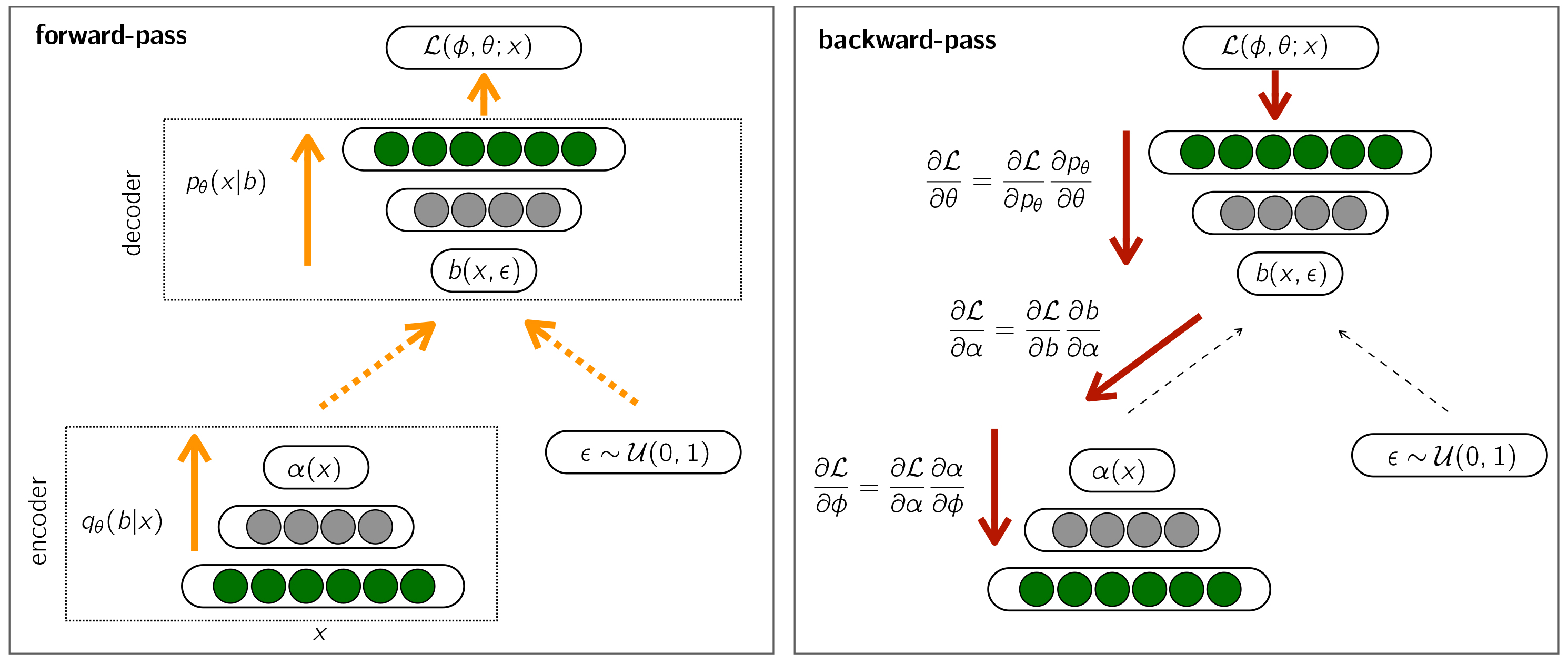

We illustrate in Fig. 2 the neural net architecture that implements our method. As other VAEs [19], it can be easily trained with vanilla back-propagation. In the forward pass, we take an input $\bm{x}^{(\ell)}$ and perform the following steps:

Compute $\alpha(\bm{x}^{(\ell)})$ using the encoder $q_{\phi}(\bm{b}|\bm{x}^{(\ell)})$ .

Simulate uniform noise $\epsilon$ to compute the sample $\hat{\bm{b}}_{\cdot,\ell}$ as in Eq. (5).

Pass the result to $g(\hat{\bm{b}}_{\cdot,\ell};\theta)$ in order to obtain the net’s output $p_{\theta}(\bm{x}^{(\ell)}|\bm{b})$ .

During the backward-pass, skipping the stochastic layers, we perform the following steps:

Compute the gradient of Eq. (4) with respect to the net’s output.

Back-propagate the error signal through the decoder parameters $\theta$ .

Back-propagate the error signal through the encoder parameters $\phi$ .

4.7 Hashing

As our model is stochastic, a straightforward use of the encoder $q_{\phi}(\bm{b}|\bm{x})$ to obtain hash codes would involve sampling. The choice $\bm{b}\sim\text{Ber}(\alpha(\bm{x}))$ guarantees that this procedure leads always to binary codes. A discretization is no required. However, in practice one may prefer deterministic codes. In that case, we can take the expected value of the stochastic representation $\alpha(\bm{x})$ and compute $\bm{b}=\bm{1}(\alpha(\bm{x})-0.5)$ , where the threshold value $0.5$ is consistent with the model’s priors. The quantization procedure applied here does not degrade significantly the codes learn by our model, because, during training, the learned codes saturates around 0/1 by the use of a Gumbel-Softmax approximation instead of other continuous relaxations (e.g. Gaussian, or Sigmoid). As shown in Fig. 1, the quantization of a Gumbel-Softmax at low temperatures is very close to the original codes i.e. it leads to a low quantization error.

To provide additional intuition about the robustness of a Bernoulli latent representation to the quantization step, we compare in Fig. 3 the distances between the representations before thresholding (using the Euclidean distance) and after thresholding (using the Hamming distance), computed on samples drawn different distributions. We can observe that Gumbel-Softmax samples at low temperature lead to similarities well correlated before and after thresholding. That means that the distance scores are preserved on the representation space after quantization. Indeed, this contrasts with samples drawn from the Gaussian distribution employed by the Gaussian variational encoder. This suggests that a Bernoulli VAE is well suited for hashing, even substituting sampling by a thresholding operation to obtain deterministic codes.

5. Experiments

We evaluate our method on text and image retrieval tasks, previously used to assess hashing algorithms [5, 24]. First we adopt the Gaussian variational autoencoder recently proposed in [5] as our main baseline (VDSH). We then extend the comparison to non-variational methods.

Table 1
Information of the data used for the evaluation of objects retrieval

	Newsgroup	Reuters	TMC	Snippets	MNIST	CIFAR-10	NUS-WIDE
Objects ( $n$ )	18,846	10,788	28,282	12,340	70,000	60,000	158,383
#Features ( $\|V\|$ or $d$ )	10,000	7,164	20,000	10,000	512	512	512
Tags/classes	20	90	22	8	10	10	21

Figure 3.

Euclidean distance before quantization (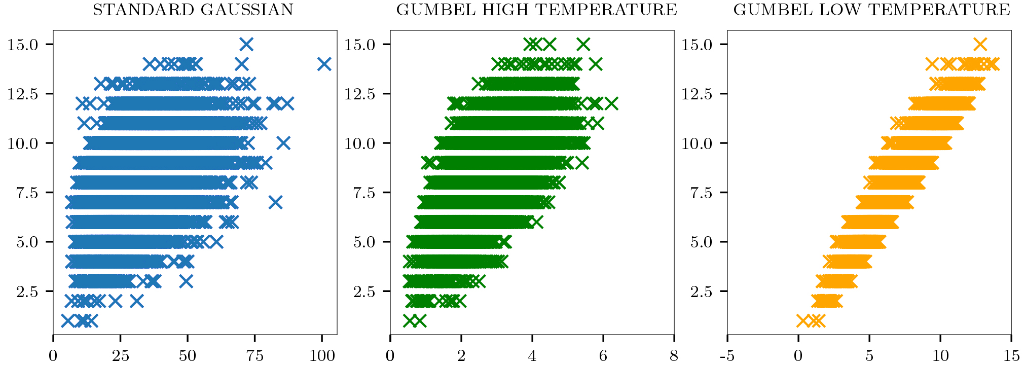 $x$ -axis) and Hamming distance after quantization ( $y$ -axis), computed on pairs of samples drawn from different latent distributions (32-bits).

5.1 Text datasets

We define four well-known text datasets: 20 Newsgroups, containing 18000 long documents (newsgroup posts) organized into 20 mutually exclusive classes; Reuters21578, containing 11000 news documents annotated with 90 non-exclusive tags (topics); TMC, containing 28000 documents (air traffic reports) organized into 22 non-exclusive tags; and Google Search Snippets, with 12000 short documents organized into 8 mutually exclusive classes (domains). These datasets were selected to experiment with documents of different length. The first three datasets have used in [5] to demonstrate the ability of standard VAEs to learn hash codes. The latter has been used in [51] with convolutional neural nets with the same purpose.

Pre-processing. We follow the pre-process setting of the work in [5]. This corresponds to perform lower-casing, removing extra-spaces, and finally removing stop-words and any character that is not a letter. The $V$ most frequent tokens are used to get a tf-idf document representation. This representation normalizes the term frequency factor $\text{tf}_{\text{w}}$ if the token $w$ appears in many documents, multiply by $\text{idf}_{\text{w}}=\log{\left(|D|/\text{df}_{w}\right)}+1$ , with $\text{df}_{w}$ the number of documents that contains $w$ . In [5], it is shown that a change in the representation (tf or binary) does not lead to significantly different results. A common training/validation/test split was done over each dataset, creating subsets of (80/10/10)% documents respectively. The pre-processed datasets and VDSH code are publicly available.1

¹
github.com/unsuthee/VariationalDeepSemanticHashing.

Neural Net Architecture. We adopt the same architecture for the encoder and decoder of the VAE baseline proposed in VDSH [5]: two fully connected (fc) layers for the encoder, with 500 ReLU activation units, and a linear decoder, with $V$ units with softmax activation. This architecture can be summarized as inp $V$ -fc500-fc500-fc $B$ -fc $V$ ( $B$ is the number of bits) using notation common in deep learning works. We also include a Batch Normalization[16] layer after each layer on the encoder. Earlier experiments reveal that this modification helps to stabilize the optimization, taking 30 epochs to converge.

The value of weight $\beta$ for the KL divergence in Eq. (7), is searched over a exponential grid ( $2^{-p}$ ) using the validation set to measure performance. The values found and set for our proposal on each dataset are $\{2^{-6},2^{-17},2^{-12},2^{-6}\}$ for 20 Newsgroups, Reuters, TMC and Snippets respectively. For the VDSH baseline these values are $\{2^{-4},2^{-4},2^{-4},2^{-3}\}$ .

5.2 Image datasets

We selected three widely-use image datasets: MNIST,2

²
http://yann.lecun.com/exdb/mnist.

containing 70000 28

\times

28 gray-scale images of handwritten digits, from 0 to 9 (10 classes); CIFAR-10,3

http://www.cs.toronto.edu/kriz/cifar.html.

containing 60000 32

\times

32 RGB images organized into 10 classes: NUS-WIDE,4

⁴

https://lms.comp.nus.edu.sg/wp-content/uploads/2019/research/nuswide/NUS-WIDE.html.

where we collected 169500 images from the original dataset in Flickr. The RGB images are annotated with 81 non-exclusive binary concepts (semantic labels). As a common setting on NUS-WIDE [39, 9], we selected the 21 most frequent labels for evaluation (158383 images).

Pre-processing. We follow the common approach of representing images based on VGGNet[42] descriptors. That means that we perform a forward pass with the re-scaled images (224 $\times$ 224) over the convolutional operations of VGG-16. This fixed-size representation helps to encode and reconstruct a simple representation of the image into a $d$ -dimensional vector. We perform the standard normalization of this representation, which consists in substracting the mean and dividing by the standard deviation. As a widely-used setting to create the test set on image datasets [24, 8, 39, 9], we randomly select 100 images from each class or tag. The validation set is created with the same procedure, keeping the rest of data to learn the proposed autoencoder.

Neural Net Architecture. We adopt an architecture similar to the one used for text hashing. As, after the convolutional layers of VGG-16, the images are fixed-size vectors, the architecture for the encoder is the same: two fully connected layers with 500 ReLU units followed of Batch Normalization. For the decoder, we set a linear layer with $d$ units (no activation) inspired in previous work [8]. This architecture can be summarized as inp $d$ -fc500-fc500-fc $B$ -fc $d$ ( $B$ is the number of bits). This model also took almost 30 epochs to converge.

The value $\beta$ for the KL in the Eq. (8) is searched in the same way as for the text datasets. The values found and set for each dataset in the experimentation are $\{2^{-16},2^{-8},2^{-9}\}$ for MNIST, CIFAR-10 and NUS-WIDE respectively. For the VDSH baseline, these values are $\{2^{-17},2^{-17},2^{-17}\}$ .

5.3 Evaluation protocol

The trained encoders are used to embed the corpus into the Hamming space. Based on this embedding, each test or validation document was then provided to the system as a query and used to retrieve similar documents from the training set. We consider two querying methods: (1) top- $K$ : retrieve $K$ documents whose hash codes are the most similar to the hash of the query, and (2) ball search: retrieve all the documents at a Hamming distance of at most $\theta$ bits. The results are evaluated using precision ( $P$ ) and recall ( $R$ ) over the retrieved documents at position $K$ . The formula for a query $q$ is given by:

$\displaystyle P_{q}@k=\frac{s_{k}}{k}\ \ \ \ \ \ \ \ \ \ R_{q}@k=\frac{s_{k}}{% |D_{q}|}\ ,$

with $D_{q}(\subseteq D)$ is the set of actual relevant documents of a query $q$ in the source dataset $D$ and $s_{k}(\leqslant|D_{q}|)$ is the number of similar document to the query $q$ among the $k$ retrieved documents. Two items were considered similar if they have at least one label in common [5].

Meanwhile, for the image datasets we also calculated the mean average precision (MAP) [37] of the Hamming ranking as several recent works do [24, 8, 39]. This metric represents an overall measurement of the retrieval performance. Let $\textit{rel}_{q}(k)$ be equal to 1 if the object at position $k$ is similar to the query $q$ (i.e. relevant). The MAP is thus given by

$\displaystyle\textit{MAP}=\frac{1}{|Q|}\sum_{q\in Q}\frac{1}{|D_{q}|}\sum_{k=1% }^{K}P_{q}@k\cdot\textit{rel}_{q}(k)\ .$

5.4 Convolutional features for image representation

Table 2
Precision and recall on the validation set using the first querying mechanism (top-100) on the MNIST dataset. The best result are bolded

Method	Representation	4 bits	8 bits	16 bits	32 bits	4 bits	8 bits	16 bits	32 bits
		Precision				Recall
VDSH	Raw	0.209	0.481	0.614	0.723	0.003	0.007	0.009	0.011
	VGG	0.310	0.536	0.664	0.770	0.004	0.008	0.010	0.011
B-VAE	Raw	0.371	0.601	0.743	0.825	0.004	0.008	0.010	0.012
	VGG	0.392	0.611	0.747	0.826	0.006	0.009	0.011	0.012

On Table 2, we can see the effect of using the VGG descriptors instead of the raw pixels in the MNIST dataset. The difficulty of using the raw pixels comes from the many parameters that encoder and decoder had to learn if trained from scratch. Here, it can be seen that the VGG representation outperforms the raw representation for all the bits and all the methods. As for the recall, the VGG representation is uniformly better, except for 32 bits where the raw representation performs equal. This experiment illustrate the effectiveness of convolutional layers to extract visual features and the advantage of using pre-trained models to reduce the number of trainable parameters.

5.5 Bernoulli versus Gaussian representations for information retrieval

In this section we compare the performance of Gaussian (VDSH, [5]) versus Bernoulli (proposed) variational autoencoders for hashing. As stated before, we present results in text and image datasets using the two querying mechanisms usually adopted in the literature.

5.5.1 Results for top $K$ Searches on image and text data

Table 3
Precision and recall on the test set using the first querying mechanism (top-100) by different number of bits. The best method on each bit configuration is bolded

		Precision				Recall
Dataset	Method	4 bits	8 bits	16 bits	32 bits	4 bits	8 bits	16 bits	32 bits
Newsgroup	VDSH	0.190	0.371	0.479	0.536	0.025	0.049	0.064	0.072
	B-VAE	0.219	0.375	0.551	0.564	0.029	0.050	0.074	0.076
Reuters	VDSH	0.510	0.681	0.731	0.773	0.028	0.042	0.049	0.058
	B-VAE	0.455	0.639	0.762	0.803	0.021	0.036	0.054	0.063
TMC	VDSH	0.582	0.650	0.682	0.703	0.007	0.010	0.012	0.013
	B-VAE	0.544	0.636	0.702	0.724	0.006	0.009	0.013	0.014
Snippets	VDSH	0.206	0.314	0.422	0.479	0.017	0.025	0.034	0.039
	B-VAE	0.156	0.345	0.483	0.517	0.012	0.029	0.040	0.045
MNIST	VDSH	0.296	0.553	0.695	0.776	0.004	0.008	0.010	0.011
	B-VAE	0.362	0.654	0.757	0.842	0.005	0.009	0.011	0.012
CIFAR-10	VDSH	0.307	0.393	0.468	0.500	0.005	0.007	0.008	0.008
	B-VAE	0.325	0.436	0.494	0.548	0.006	0.007	0.008	0.009
NUS-WIDE	VDSH	0.560	0.659	0.726	0.766	0.001	0.001	0.001	0.002
	B-VAE	0.594	0.668	0.740	0.776	0.001	0.001	0.001	0.002

In Table 3, we compare the results obtained by the Gaussian [5] and Bernoulli autoencoders using the first querying mechanism, for different number of bits $B$ . In terms of precision, our method outperforms the traditional VAE in all the image datasets and independently of the number of bits. In these datasets, our method has also an advantage in terms of recall in most cases, except for some particular configurations (e.g. 8 and 16 bits in CIFAR-10) where both methods perform equally well. In the text datasets, our proposed method maintains the advantage in precision and recall when we have enough number of bits ( $B\geqslant$ 16), except on the Newsgroup dataset where our method outperforms the Gaussian autoencoder in all the cases. If we use 4 bits, both methods suffer a high impact in terms of performance but the baseline gets more precise. We attribute this to the selected prior, that expects the entropy of the different bits to be high to prevent overfitting. It should be noted that, as word sizes are typically determined using bytes, using 4 bits is pretty uncommon in the literature.

In summary, our variational autoencoder outperforms the more traditional Gaussian autoencoder in terms of precision and recall in most cases. We achieved some large gaps of improvement on some cases. For instance, using 16 bits, the precision of the proposed method is $\sim$ 15% better on Newsgroup and $\sim$ 14% better on Snippets. Using 8 bits, it is $\sim$ 18% better in MNIST and $\sim$ 10% in CIFAR-10. This demonstrates the practical advantage of using explicit Bernoulli latent variables for hashing.

Table 4

MAP on the test set using all the hamming ranking by different number of bits. Best method on each bit configuration is on bold

Dataset	Method	4 bits	8 bits	16 bits	32 bits
Newsgroup	VDSH	0.155	0.233	0.306	0.375
	B-VAE	0.214	0.277	0.393	0.376
Reuters	VDSH	0.444	0.575	0.528	0.588
	B-VAE	0.425	0.508	0.619	0.604
TMC	VDSH	0.518	0.525	0.543	0.556
	B-VAE	0.514	0.540	0.560	0.558
Snippets	VDSH	0.177	0.243	0.280	0.300
	B-VAE	0.157	0.272	0.306	0.330
MNIST	VDSH	0.267	0.349	0.372	0.392
	B-VAE	0.304	0.471	0.505	0.516
CIFAR-10	VDSH	0.230	0.254	0.236	0.250
	B-VAE	0.250	0.287	0.278	0.271
NUS-WIDE	VDSH	0.529	0.510	0.520	0.515
	B-VAE	0.519	0.537	0.549	0.552

In Table 4, we compare the test performance of the methods in terms of mean average precision (MAP) overall hamming ranking. The obtained results are similar to those remarked previously in terms of ranked precision, i.e. our method outperforms the MAP of the baseline in most cases (bits) on the different datasets. In some datasets (Newsgroup, MNIST and CIFAR-10), our method is the best independently of number of bits (4 cases), while in other cases it is better in most of them (3 against 1 in TMC, Snippets and NUS-WIDE). In the Reuters dataset, the results are more evenly split between the algorithms: our method outperforms the baseline in only two cases. Overall, these results show that the proposed method maintains its advantages when the ranking on the whole dataset is considered. Sometimes we observe large gaps of improvement. For instance, the MAP of our method is $\sim$ 38% better using 4 bits in Newsgroups, $\sim$ 17% better with 16 bits in Reuters and $\sim$ 12% better with 8 bits in Snippets. On the image datasets, we achieved a $\sim$ 35% improvement with 8 and 16 bits in MNIST and $\sim$ 18% with 16 bits in CIFAR-10.

5.5.2 Results for range searches on image and text data

Figure 4.

Precision (circles) and recall (triangles) using the second querying mechanism (ball search), 32 bits are used. Points are obtained using different values of 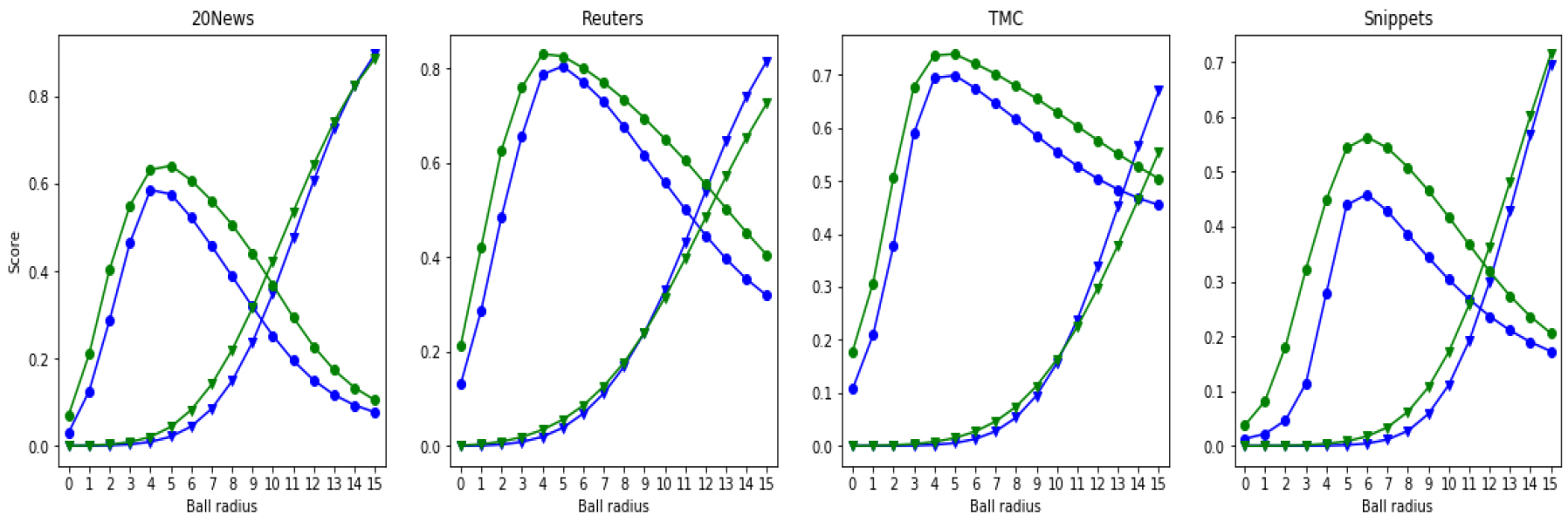$\theta$ on the text datasets. Upper curves for our method (B-VAE) and lower curves are for the baseline (VDSH).

In Fig. 4, we show the performance obtained by both types of autoencoder on the text datasets using the second querying mechanism, ball search. We fix the number of bits of the codes to 32 and vary, as usual, the value of search parameter (radius) $\theta$ . Results show that the advantage of the proposed method is robust to the choice of the search radius which is problem dependent and thus need to be carefully tuned in real world applications. The proposed method obtains a better precision in all the cases. As for the recall, it is more even among the algorithms.

Figure 4 also illustrates the advantage of using the second querying mechanism instead of the first one. For example, using $\theta=$ 8 (bits) in Reuters, our method can increase the recall from $\sim$ 0.06 (Table 3) to $\sim$ 0.20 without significantly reducing the precision. Using $\theta=$ 6 (bits) in Snippets, our method can increase the precision from 0.52 to $\sim$ 0.60, keeping the advantage in terms of recall. These results suggest the following interpretation about the encoding function learned by the models. In Reuters and TMC, the precision increases with a higher slope. That means that similar objects are very close in the Hamming Space while dissimilar objects are very far. The number of true positives increases quickly with a slight increase in the search radius without significantly increasing the number of false positives. In Snippets one has to explore more the space (change more bits) to find similar objects.

Figure 5.

Precision (circles) and recall (triangles) using the second querying mechanism (ball search), 32 bits are used. Points are obtained using different values of 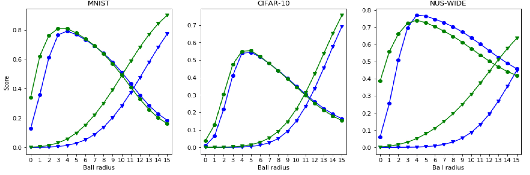$\theta$ on the image datasets. Comparison between our method (B-VAE) and baseline (VDSH). The curves that are greater at radius zero are from B-VAE.

In Fig. 5, we show the results obtained in the image datasets. Conclusions are similar to those drawn from the previous experiments. The proposed method obtains a better precision and recall in most cases, being the recall the metric that gets a more clear improvement. Also, based on same criteria commented earlier, it can be seen that in MNIST and NUS-WIDE, similar objects are very close in Hamming space. In CIFAR-10 one has to explore more the Hamming space to find similar objects.

5.6 Variational versus non-variational methods for hashing

5.6.1 Text retrieval tasks

We use the same experimental setting of [5], same datasets and evaluation protocol, in order to compare the variational methods against other unsupervised techniques for text hashing: LSH [7] (data-independent method) SH [50] (popular shallow baseline) and Stacked RMBs [38] (deep graphical model).

Table 5
Precision on the test set using the first querying mechanism (top- $100$ ). Values are extracted from [5]. The VDSH ${}^{\star}$ stands for our own implementation of the VDSH model. Best result on each dataset and bit is presented in bold

Dataset	Method	8 bits	16 bits	32 bits
Newsgroup	LSH [7]	0.057	0.060	0.067
	SpH [50]	0.255	0.320	0.371
	Stacked RBMs [38]	0.059	0.060	0.053
	VDSH [5]	0.364	0.390	0.433
	VDSH ${}^{\star}$	0.371	0.479	0.536
	B-VAE	0.375	0.551	0.564
Reuters	LSH [7]	0.280	0.322	0.386
	SpH [50]	0.608	0.634	0.651
	Stacked RBMs [38]	0.511	0.574	0.615
	VDSH [5]	0.686	0.717	0.775
	VDSH ${}^{\star}$	0.681	0.731	0.773
	B-VAE	0.639	0.762	0.803
TMC	LSH [7]	0.439	0.439	0.451
	SpH [50]	0.581	0.606	0.628
	Stacked RBMs [38]	0.485	0.511	0.517
	VDSH [5]	0.433	0.685	0.711
	VDSH ${}^{\star}$	0.650	0.682	0.703
	B-VAE	0.636	0.702	0.724

The results are presented in Table 5. First, it is worth noting that our own implementation of the Gaussian variational autoencoder (VDSH) obtains slightly better results in most cases. This could be due to the parameter used to weight the KL divergence in the objective function used for training that is selected using a validation set.

The results in Table 5 show that the variational (stochastic) models are better for hashing and information retrieval than the classic shallow models and the deep generative baseline. In most cases, the Bernoulli autoencoder outperforms all the unsupervised methods. In the Newsgroups dataset, this advantage is independent of the number of bits, while on Reuters and TMC our method outperforms all the baselines using 16 and 32 bits. With 8 bits, the proposed method is the second best performer after the VDSH method. Overall, these results show that a variational autoencoder with Bernoulli latent variables is an effective technique for text hashing, often providing state of the art performance.

5.6.2 Image retrieval tasks

We use the same setting of [39], same datasets and evaluation protocol, in order to compare against more unsupervised hashing techniques specialized on image retrieval. Here we compare the Bernoulli autoencoder against: LSH [7], SH [50], ITQ [11], and UH-BDNN [8], a state-of-the-art deterministic autoencoder model. All the methods use VGG convolutional descriptors.

Table 6
MAP on hamming ranking and Precision at 5000 on test set retrieval. Values are extracted from [39]. The VDSH ${}^{\star}$ stands for our implementation of the VDSH model. Best results on each bit and dataset are presented in bold. All methods use VGG descriptors

		MAP		P@ $k=$ 5000
Dataset	Method	16 bits	32 bits	16 bits	32 bits
MNIST	LSH [7]	0.167	0.182	0.195	0.244
	SpH [50]	0.249	0.241	0.299	0.296
	ITQ [11]	0.238	0.289	0.279	0.335
	UH-BDNN [8]	0.358	0.384	0.404	0.429
	VDSH ${}^{\star}$ [5]	0.372	0.392	0.428	0.454
	B-VAE	0.505	0.516	0.557	0.573
CIFAR-10	LSH [7]	0.151	0.166	0.204	0.259
	SpH [50]	0.209	0.189	0.242	0.224
	ITQ [11]	0.242	0.267	0.271	0.300
	UH-BDNN [8]	0.301	0.309	0.340	0.345
	VDSH ${}^{\star}$ [5]	0.236	0.250	0.273	0.290
	B-VAE	0.278	0.271	0.313	0.308
NUS-WIDE	LSH [7]	0.405	0.480	0.480	0.553
	SpH [50]	0.447	0.426	0.592	0.550
	ITQ [11]	0.543	0.548	0.673	0.689
	UH-BDNN [8]	0.543	0.517	0.702	0.696
	VDSH ${}^{\star}$ [5]	0.520	0.515	0.659	0.667
	B-VAE	0.549	0.552	0.680	0.697

The results on the image datasets, comparing MAP and Precision at top-5000, are presented in Table 6. Here it can be seen that the variational Gaussian autoencoder (VDSH) outperforms classic shallow models only on MNIST, being competitive against ITQ model in CIFAR-10 and NUS-WIDE. However, the proposed model is better than all the shallow models, in all the datasets and considering both retrieval metrics (MAP and ranked precision). Furthermore, the Bernoulli autoencoder is the best among all the methods (shallow and deep) in the MNIST dataset (MAP and ranked precision) and partially in NUS-WIDE (only MAP). The deep deterministic autoencoder (UH-BDNN) is competitive with the variational autoencoders on all the datasets: it exhibits the best MAP and ranked precision in CIFAR-10 and the best precision in NUS-WIDE, where our method is the second best option.

In summary, our B-VAE method shows the best MAP on 2 of 3 datasets and deep deterministic autoencoder presents the best precision on 2 of 3 datasets. Obtaining a good MAP is something commonly desired in image retrieval applications [8, 39, 9], because it considers the order of the search results. The better MAP scores of the Bernoulli autoencoder indicates that it puts more relevant documents on the top of the list.

As earlier experiments shows, our proposal is often the best among the variational models. However, the results in Table 6 shows that there is no a uniform winner in image hashing. It depends on the dataset type and the metric used to assess the models (e.g. MAP or ranked precision).

5.7 Interpretation of the hash codes

Table 7
Examples of most probable words by activating a bit on the hash code

Newsgroup	Reuters	Snippets
bit 9	bit 31	bit 25
Complexity	Device	Interaction
Heterosexual	Recognize	Biogeography
Likelihood	Responsibility	Composer
Inconsistent	Analyze	Radiology
Skeptic	Printing	Gymnastics
Presidential	Undoubtedly	Patient
Prohibits	Describing	Ballet
Homosexuality	Projecting	Strength

As the proposed method uses binary latent variables, each factor of the latent representation learned by this model can be understood as a bit of the address assigned to data point in the Hamming space. To show that this interpretation offers practical advantages, we conduct experiments aimed to analyze the properties of the codes learned by the model.

As a first experiment, we use the decoder (generator) learned on the text datasets, to determine if the bits can be assigned a semantics as in topic models used for text mining. As the reconstruction layer computes a probability distribution over the words/tokens, we can activate a single bit of the hash code and compute the top most probable words generated by the decoder. Table 7 shows a selection of the results of this experiment. We can see that in Newsgroups, bit number 9 seems to detect political discussions regarding sexuality. In Reuters, bit number 31 captures computer-related concepts. In Snippets, bit number 25 seems to detect terms associated with health or sport.

As a second experiment we use the encoder of the variational autoencoders to inspect the properties of the representation learned by these modes. Figure 6 shows histograms of the representations generated by both methods in the text datasets. For the Gaussian autoencoder we show the expectation $\mu(\bm{x})$ corresponding to the latent layer. Figure 7 shows equivalent graphs for the image datasets. For the Bernoulli autoencoder we show the activation probabilities $\alpha(\bm{x})$ corresponding to different factors/bits averaging among the different bits. In the graphs labelled by $\alpha(\bm{x})$ , the histograms were computed without averaging $\alpha(\bm{x})$ among the data points and considering all the bits. In the graphs labelled by $\alpha_{i}(\bm{x})$ , we plot the marginal activation probability of each bit separately, after averaging among the data i.e. we compute an histogram of $\mathbb{E}_{x}[\alpha_{i}(\bm{x})]$ .

Figure 6.

Histograms of the representations learned by B-VAE and VDSH (activation probabilities and mean values respectively) in the 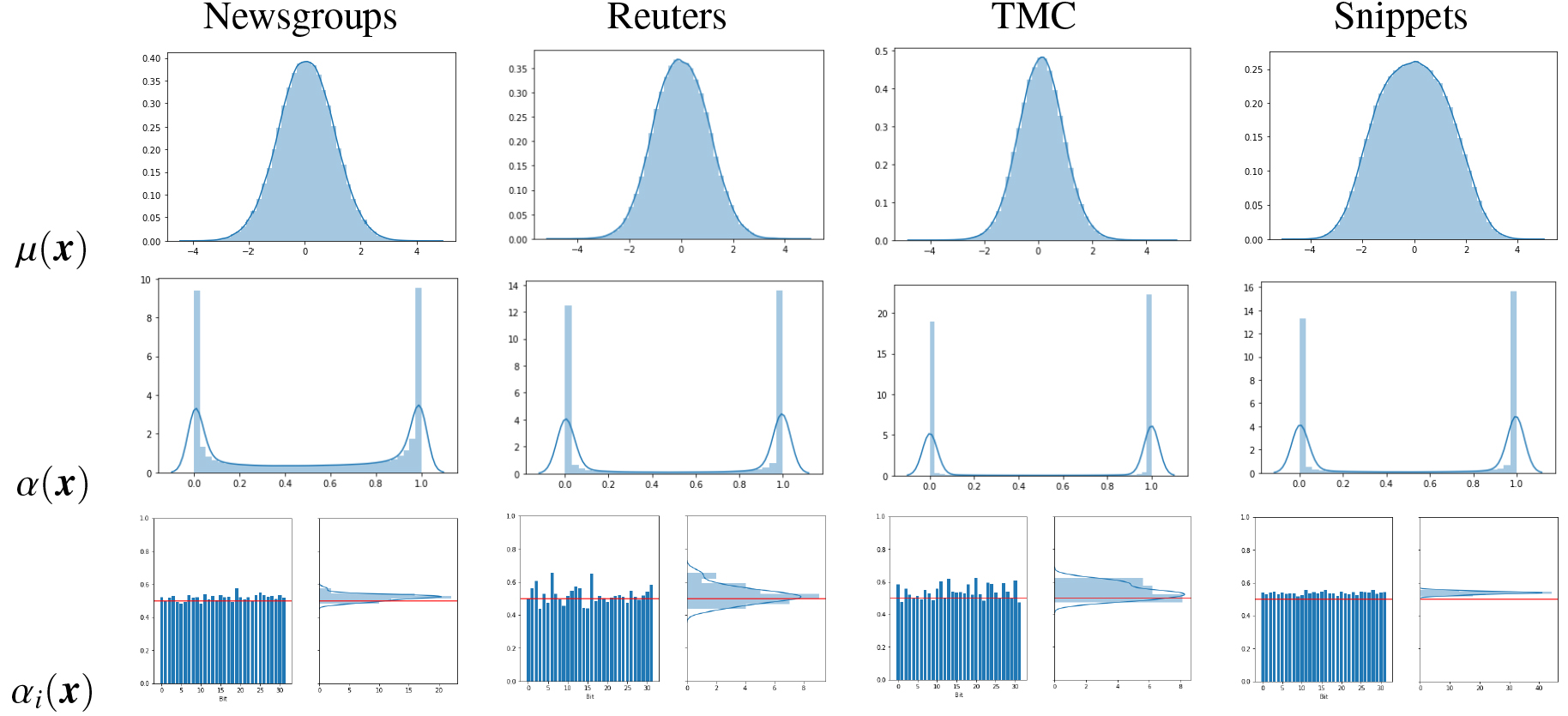text datasets. Last row shows the average of probability activation. For both methods we used a code length of $B=$ 32.

It can be seen that the activation probabilities of the bits learned for every object $x^{(\ell)}$ are saturated at the extremes (0 or 1), as expected. This is a good property, as we want to reduce the quantization error introduced by the thresholding operation applied to obtain deterministic codes. In average, the learned probabilities are very certain of the bit activation. Rephrasing, the model learns that some bits have to be ON for some inputs and have to be OFF for others, but it is unlikely that the model does not known if activating the bit or not. The figure also illustrates the lack of interpretability of the continuous representation learned by the Gaussian autoencoder. The representation cannot be easily associated to the bits using for indexing and search.

By inspecting the marginal activation probabilities in text datasets (Fig. 6), it can be seen another good property of the proposed model: the average activation probability is close to 0.5. As the activations are saturated at the extremes, that implies that every bit is 1 for about half of the dataset and 0 for the other half and so practically every bit is used to discriminate/separate. On the image datasets (Fig. 7) we observe a different result. For example, in the MNIST and NUS-WIDE datasets, some bit averages are very close to 1 and other very close to 0. That means that in these cases, some bits practically do not change their values. This perhaps explains why in these datasets, the proposed method is not always the top performer, and suggests that there is room for improvement in the design of the objective function.

5.8 Effect of tresholding

Figure 7.

Histograms of the representations learned by B-VAE and VDSH (activation probabilities and mean values respectively) in the 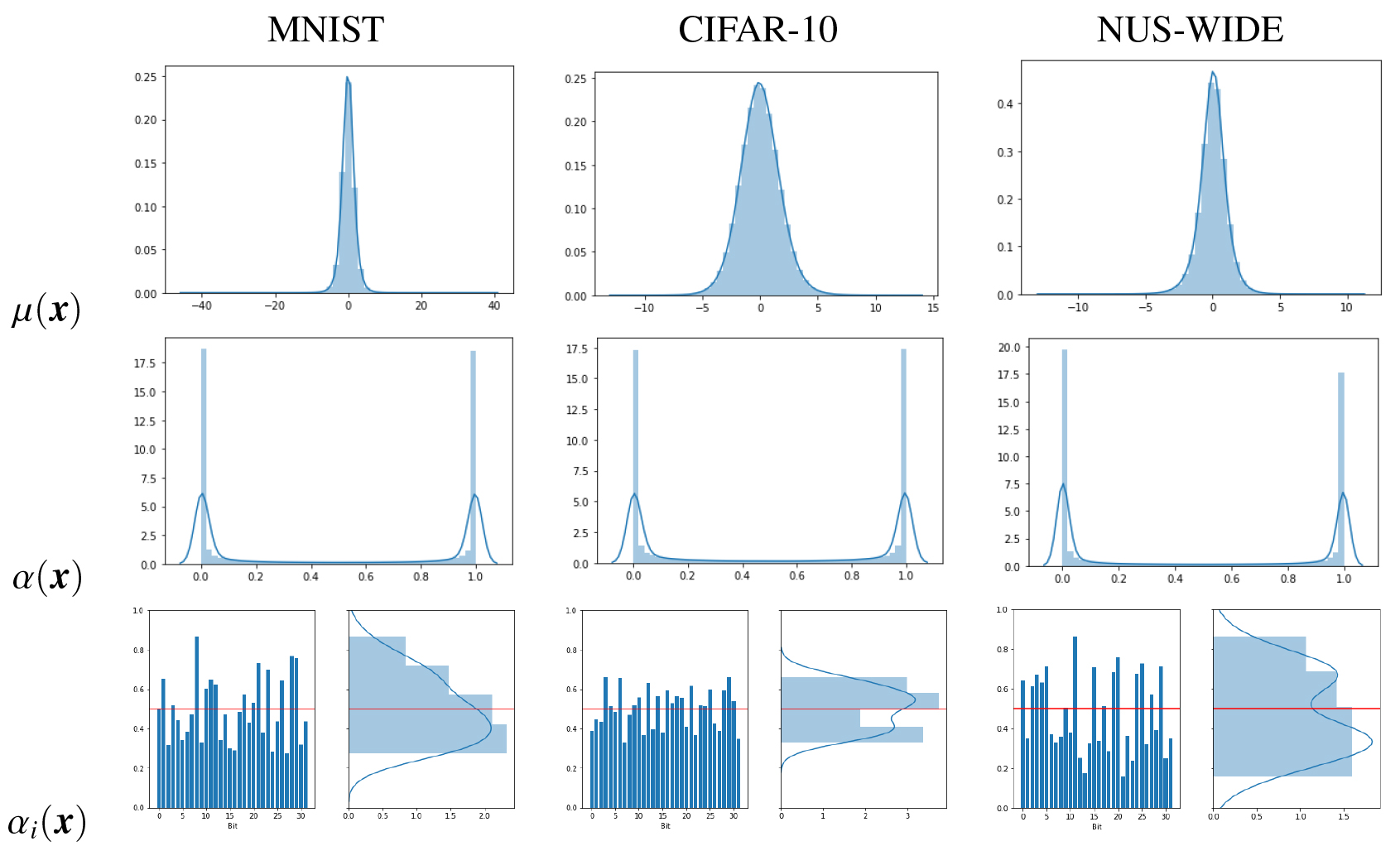image datasets. Last row shows the average of probability activation. For both methods we used a code length of $B=$ 32.

To analyze the effect of quantization on the representations learned by the traditional and the proposed autoencoder, we conduct extrinsic evaluation experiments which use classification as the desired (in this case auxiliary) task. To this end, we use a shallow fully connected network with one hidden layer of 256 ReLU units and a Softmax output layer that predicts the classes or tags corresponding to the input pattern.

Our first goal is to determine if a continuous (Gaussian) representation has advantages before thresholding (binarization). Hence, we first use the encoders of the Gaussian and the Bernoulli models to represent the data, train the neural net on these representation, and evaluate the accuracy and Jaccard score of the classifier on the training and test sets. The first column of Table 8 presents the results for a code length of 32 bits. We can see that the baseline (VDSH) obtains always the best performance, except in the test set of Snippets. This advantage is completely expected because the Gaussian model is trained to preserve information about the data in the form of a continuous embedding while the Bernoulli model constraints the latent variables to have only two states.

Table 8

Performance of labels prediction on training and test set, using the representation with 32 bits obtained before and after thresholding. Accuracy and Jaccard score for unique and multi label datasets. Best results on each set are presented in bold

		Before thresholding		After thresholding		Before $\rightarrow$ After
Dataset	Method	Train	Test	Train	Test	Train	Test
Newsgroup	VDSH	84.59	79.01	75.15	70.50	43.26	41.60
	B-VAE	83.15	77.13	80.41	73.23	79.07	73.01
Reuters	VDSH	79.55	77.41	72.60	70.05	36.31	35.68
	B-VAE	74.44	72.55	73.75	71.39	73.86	71.04
TMC	VDSH	53.60	46.31	49.60	42.97	31.57	28.72
	B-VAE	53.02	45.44	53.13	44.58	52.68	44.59
Snippets	VDSH	89.47	65.48	82.53	61.05	48.96	31.93
	B-VAE	89.06	68.20	87.92	66.23	87.43	65.79
MNIST	VDSH	97.94	95.40	90.63	88.30	49.95	51.50
	B-VAE	93.66	92.50	91.41	91.10	90.71	90.50
CIFAR-10	VDSH	87.65	84.90	74.18	73.00	44.06	42.80
	B-VAE	78.88	77.10	75.38	74.30	74.31	73.80
NUS-WIDE	VDSH	53.58	49.02	44.73	38.61	30.55	28.23
	B-VAE	48.24	41.64	44.63	37.79	45.26	38.74

We now binarize the data representation of both methods using the thresholding operation required to obtain hash codes, and repeat the procedure of training and evaluating the neural net. The second column of Table 8 summarizes the results. We can see that the superiority of the continuous Gaussian representation is lost after thresholding. The representation learned by our model outperforms the baseline in most cases (except NUS-WIDE) on the training and test sets. In addition, we can see that the Bernoulli representation has quite similar performance before and after thresholding. This is very clear in Reuters, TMC, Snippets and NUS-WIDE. We can conclude that (i) using Bernoulli latent variables the representation learned by the model is practically the same before and after thresholding; (ii) as the Bernoulli autoencoder learns to preserve the information about the dataset in the form of bits, it has advantages over a model trained to preserve that information in the form continuous features, when binary codes are required.

We conducted a additional experiment in which we train the classifier using the raw representations computed by the encoder but test the model using the representation after thresholding. The last column of Table 8 presents the results (“before $\rightarrow$ after” column). From this experiment we confirm that the representations of our model before and after thresholding are practically the same: the patterns learned to discriminate the classes are more robust to the quantization step.

Altogether, the results obtained in this section confirm that a standard variational autoencoder has an advantage if a continuous representation is required, but the Bernoulli VAE that we propose (B-VAE) is better suited for applications where a binary representation is required, as in indexing and search using hash codes.

6. Conclusions and final remarks

In this paper we have approached the problem of hashing in the framework of variational autoencoders and deep learning. This led to a novel algorithm to learn hash codes that resorts to an auxiliary generator network to compensate the lack of a supervisor. In contrast to methods based on traditional autoencoders, the model is not trained to learn a query-code association deterministically. Instead, an encoder network predicts the most likely region of the Hamming space where the input pattern could be allocated, in such a way that the generator net can reconstruct the observation by sampling from that region.

Our model for hashing differs from a previous technique using variational autoencoders by a simple but crucial decision: the latent codes are constrained to be binary. This is achieved by imposing Bernoulli instead of Gaussian distributions to the encoder, which leads to a model more easy to interpret in the context of hashing. The implementation and experimental analysis that resulted from this research proved that the latter choice is not problematic in a computational sense. The reparametrization trick is an effective technique to perform backpropagation through Bernoulli random layers and no specialized solvers are required.

We have assessed the proposed technique using seven public datasets from two different domains, namely image and text data, comparing the results with various methods from the state of the art. We found that learning Bernoulli rather than Gaussian latent variables improves similarity search metrics in the large majority of cases. In image retrieval tasks, the proposed method outperformed the Gaussian variational autoencoder in all the cases. A deterministic autoencoder with active binary constraints showed better ranked precision in many cases, suggesting than there is no silver bullet for hashing. As in these experiments, the proposed model provided the second best result, we can conclude that a Bernoulli autoencoder is a robust technique for hashing image data, even if sometimes it is not the top performer. Experiments on document retrieval tasks on the other hand, showed that in most cases the proposed method outperforms the Gaussian variant also in this type of problems. Together, the variational autoencoders were found always more effective than other techniques from the state of the art. Overall, these experiments demonstrated that the proposed method is functionally flexible and can be adapted to different types of data - it is enough to specialize the architecture of the neural nets for a particular application.

Experiments to illustrate the interpretability of the proposed model were also performed using the encoder and the decoder. In the text datasets, we found that most bits of the code learned by the model can be associated with a topic or set of words semantically related. We also found that most bits in the model are activated with a distribution that, in average, respects the model’s priors. All the bits were used to preserve information about the dataset, but they were activated selectively for some inputs but not for others. Finally, specific experiments were performed to measure the effect of quantization in both types of autoencoder. We found, as expected, that learning a continuous representation gives an advantage to the Gaussian autoencoder in tasks that do not require quantization. However, after quantization, the representations learned by the Bernoulli autoencoder preserves significantly more information about the dataset, and outperforms the Gaussian representations in all the extrinsic evaluations conducted except one (in which both perform about the same).

Overall, we conclude that Bernoulli variational autoencoders are an effective, interpretable and flexible approach to learn hash codes. In future work, we plan to extend this model to semi-supervised problems in which labels are available only for a small part of the dataset. We are also conducting experiments with novel training criteria inspired in information theory.

Footnotes

Acknowledgments

F. Mena thanks the Programa de Iniciación Científica PIIC-DGIP of the Federico Santa María University for funding this work.

References

Baeza-Yates

and Ribeiro-Neto

, Modern Information Retrieval, ACM, 1999.

Baldi

, Autoencoders, unsupervised learning, and deep architectures, In Proceedings of ICML workshop on unsupervised and transfer learning, 2012, pp. 37–49.

Broder

A.Z.

, On the resemblance and containment of documents, In Proceedings Compression and Complexity of SEQUENCES 1997 (Cat. No. 97TB100171), IEEE, 1997, pp. 21–29.

Carreira-Perpinán

M.A.

and Raziperchikolaei

, Hashing with binary autoencoders, In Proceedings of the CVPR, 2015, pp. 557–566.

Chaidaroon

and Fang

, Variational deep semantic hashing for text documents, In Proceedings of the 40th SIGIR, ACM, 2017, pp. 75–84.

Charikar

M.S.

, Similarity estimation techniques from rounding algorithms, In Proceedings of the thiry-fourth annual ACM symposium on Theory of computing, 2002, pp. 380–388.

Datar

Immorlica

Indyk

and Mirrokni

V.S.

, Locality-sensitive hashing scheme based on p-stable distributions, In Proceedings of the twentieth annual symposium on Computational geometry, 2004, pp. 253–262.

T.-T.

Doan

A.-D.

and Cheung

N.-M.

, Learning to hash with binary deep neural network, In Proceedings of the ECML, 2016, pp. 219–234.

Crémilleux

and Jurie

, Unsupervised deep hashing with stacked convolutional autoencoders, In 2017 IEEE International Conference on Image Processing (ICIP), IEEE, 2017, pp. 3420–3424.

10.

Gionis

Indyk

Motwani

et al., Similarity search in high dimensions via hashing, In Proceedings of the 25th International Conference on Very Large Data Bases, volume 99, 1999, pp. 518–529.

11.

Gong

Lazebnik

Gordo

and Perronnin

, Iterative quantization: A procrustean approach to learning binary codes for large-scale image retrieval, IEEE Transactions on Pattern Analysis Machine Intelligence 35(12) (2013), 2916–2929.

12.

Goodfellow

Bengio

and Courville

, Deep learning, MIT press, 2016.

13.

Higgins

Matthey

Pal

Burgess

Glorot

Botvinick

Mohamed

and Lerchner

, beta-vae: Learning basic visual concepts with a constrained variational framework, Iclr 2(5) (2017), 6.

14.

Chen

and Zhang

, Bayesian supervised hashing, In Proceedings of the IEEE Conference on Computer Vision and Pattern Recognition, 2017, pp. 6348–6355.

15.

Indyk

and Motwani

, Approximate nearest neighbors: towards removing the curse of dimensionality, In Proceedings of the thirtieth annual ACM symposium on Theory of computing, 1998, pp. 604–613.

16.

Ioffe

and Szegedy

, Batch normalization: Accelerating deep network training by reducing internal covariate shift, arXiv preprint arXiv:1502.03167, 2015.

17.

Jang

and Poole

, Categorical reparameterization with Gumbel-softmax, In Proceedings of the ICLR, 2017.

18.

Jia

Sun

Gao

Song

and Shi

B.E.

, Laplacian auto-encoders: An explicit learning of nonlinear data manifold, Neurocomputing 160 (2015), 250–260.

19.

Kingma

D.P.

and Welling

, Auto-encoding variational Bayes, 2013.

20.

Krizhevsky

Sutskever

and Hinton

G.E.

, Imagenet classification with deep convolutional neural networks, In Advances in neural information processing systems, 2012, pp. 1097–1105.

21.

Kulis

and Darrell

, Learning to hash with binary reconstructive embeddings, In Advances in neural information processing systems, 2009, pp. 1042–1050.

22.

Kulis

and Grauman

, Kernelized locality-sensitive hashing, IEEE Transactions on Pattern Analysis and Machine Intelligence 34(6) (2012), 1092–1104.

23.

Lin

Shen

Suter

and Van Den Hengel

, A general two-step approach to learning-based hashing, In Proceedings of the IEEE international conference on computer vision, 2013, pp. 2552–2559.

24.

Liong

V.E.

Wang

Moulin

and Zhou

, Deep hashing for compact binary codes learning, In Proceedings of the CVPR 2015, 2015, pp. 2475–2483.

25.

Lipton

Z.C.

Berkowitz

and Elkan

, A critical review of recurrent neural networks for sequence learning, arXiv preprint arXiv:1506.00019, 2015.

26.

Liu

Wang

Shan

and Chen

, Deep supervised hashing for fast image retrieval, In Proceedings of the IEEE conference on computer vision and pattern recognition, 2016, pp. 2064–2072.

27.

Liu

Wang

Jiang

Y.-G.

and Chang

S.-F.

, Supervised hashing with kernels, In CVPR 2012, 2012, pp. 2074–2081.

28.

Liu

Wang

Kumar

and Chang

S.-F.

, Hashing with graphs, 2011.

29.

Liong

V.E.

and Zhou

, Deep hashing for scalable image search, IEEE Transactions on Image Processing 26(5) (2017), 2352–2367.

30.

Maddison

C.J.

Mnih

and Teh

Y.W.

, The concrete distribution: A continuous relaxation of discrete random variables, arXiv preprint arXiv:1611.00712, 2016.

31.

Maddison

C.J.

Tarlow

and Minka

, A* sampling, In Advances in Neural Information Processing Systems, 2014, pp. 3086–3094.

32.

Mena

and Ñanculef

, A binary variational autoencoder for hashing, In Iberoamerican Congress on Pattern Recognition, Springer, 2019, pp. 131–141.

33.

Norouzi

and Fleet

D.J.

, Minimal loss hashing for compact binary codes, In Proceedings of the 28th ICML, 2011, pp. 353–360.

34.

Norouzi

Punjani

and Fleet

D.J.

, Fast exact search in Hamming space with multi-index hashing, IEEE PAMI 36(6) (2014), 1107–1119.

35.

Potapczynski

Loaiza-Ganem

and Cunningham

J.P.

, Invertible gaussian reparameterization: Revisiting the gumbel-softmax, arXiv preprint arXiv:1912.09588, 2019.

36.

Qin

Liu

and Chen

, How convolutional neural network see the world-a survey of convolutional neural network visualization methods, arXiv preprint arXiv:1804.11191, 2018.

37.

Rasiwasia

Costa Pereira

Coviello

Doyle

Lanckriet

G.R.

Levy

and Vasconcelos

, A new approach to cross-modal multimedia retrieval, In Proceedings of the 18th ACM international conference on Multimedia, 2010, pp. 251–260.

38.

Salakhutdinov

and Hinton

, Semantic hashing, International Journal of Approximate Reasoning 50(7) (2009), 969–978.

39.

Shen

Liu

Yang

Huang

and Shen

H.T.

, Unsupervised deep hashing with similarity-adaptive and discrete optimization, IEEE Transactions on Pattern Analysis and Machine Intelligence 40(12) (2018), 3034–3044.

40.

Shrivastava

and Li

, In defense of minhash over simhash, In Artificial Intelligence and Statistics, 2014, pp. 886–894.

41.

Silveira

, A. C., M. C., and M.-F. M., Topic modeling using variational auto-encoders with Gumbel-softmax and logistic-normal mixture distributions, In International Joint Conference on Neural Networks (IJCNN), IEEE, 2018.

42.

Simonyan

and Zisserman

, Very deep convolutional networks for large-scale image recognition, arXiv preprint arXiv:1409.1556, 2014.

43.

Strecha

Bronstein

and Fua

, Ldahash: Improved matching with smaller descriptors, IEEE Trans Pattern Anal Mach Intell 34(1) (2012), 66–78.

44.

Wang

Kumar

and Chang

S.-F.

, Semi-supervised hashing for scalable image retrieval, In 2010 IEEE Computer Society Conference on Computer Vision and Pattern Recognition, IEEE, 2010, pp. 3424–3431.

45.

Wang

Kumar

and Chang

S.-F.

, Semi-supervised hashing for large-scale search, IEEE Trans Pattern Anal Mach Intell 34(12) (2012), 2393–2406.

46.

Wang

Liu

Kumar

and Chang

S.-F.

, Learning to hash for indexing big data – A survey, Proceedings of the IEEE 104(1) (2016), 34–57.

47.

Wang

Liu

Sun

A.X.

and Jiang

Y.-G.

, Learning hash codes with listwise supervision, In Proceedings of the IEEE International Conference on Computer Vision, 2013, pp. 3032–3039.

48.

Wang

Zhang

and Zha

, Adaptive manifold learning, In Advances in neural information processing systems, 2005, pp. 1473–1480.

49.

Wang

X.-J.

Zhang

Jing

and Ma

W.-Y.

, Annosearch: Image auto-annotation by search, In 2006 IEEE Computer Society Conference on Computer Vision and Pattern Recognition (CVPR’06), volume 2, IEEE, 2006, pp. 1483–1490.

50.

Weiss

Torralba

and Fergus

, Spectral hashing, In NIPS, 2009.

51.

Wang

Tian

Zhao

Wang

and Hao

, Convolutional neural networks for text hashing, In Proceedings of the IJCAI’15, 2015.

52.

Yang

H.-F.

Lin

and Chen

C.-S.

, Supervised learning of semantics-preserving hash via deep convolutional neural networks, IEEE Transactions on Pattern Analysis and Machine Intelligence 40(2) (2017), 437–451.

53.

Zhang

W.-J.

and Guo

, Supervised hashing with latent factor models, In Proceedings of the 37th international ACM SIGIR conference on Research & development in information retrieval, 2014, pp. 173–182.

54.

Zhao

Huang

Wang

and Tan

, Deep semantic ranking based hashing for multi-label image retrieval, In Proceedings of the IEEE conference on computer vision and pattern recognition, 2015, pp. 1556–1564.

55.

Zhen

and Yeung

D.-Y.

, A probabilistic model for multimodal hash function learning, In Proceedings of the 18th ACM SIGKDD international conference on Knowledge discovery and data mining, 2012, pp. 940–948.

Interpretable and effective hashing via Bernoulli variational auto-encoders

Abstract

Keywords

1. Introduction

2.1 Similarity search

2.2 Hashing

2.3 Quantization error

2.4 Focus

2.5 Standard loss functions on discrete data

3.1 Randomized methods

3.2 Shallow learning based approaches

3.3 Deep learning methods

3.4 Autoencoders

3.5 Deep graphical models

3.5.1 Variational autoencoders

4. Proposed method

4.2 Learning approach

5. Experiments

Table 1 Information of the data used for the evaluation of objects retrieval

1 github.com/unsuthee/VariationalDeepSemanticHashing.

2 http://yann.lecun.com/exdb/mnist.

5.4 Convolutional features for image representation

Table 2 Precision and recall on the validation set using the first querying mechanism (top-100) on the MNIST dataset. The best result are bolded

5.5.1 Results for top K Searches on image and text data

Table 3 Precision and recall on the test set using the first querying mechanism (top-100) by different number of bits. The best method on each bit configuration is bolded

5.6.1 Text retrieval tasks

Table 5 Precision on the test set using the first querying mechanism (top- 100 ). Values are extracted from [5]. The VDSH ⋆ stands for our own implementation of the VDSH model. Best result on each dataset and bit is presented in bold

Table 6 MAP on hamming ranking and Precision at 5000 on test set retrieval. Values are extracted from [39]. The VDSH ⋆ stands for our implementation of the VDSH model. Best results on each bit and dataset are presented in bold. All methods use VGG descriptors

Table 7 Examples of most probable words by activating a bit on the hash code

Footnotes

Acknowledgments

References

Table 1
Information of the data used for the evaluation of objects retrieval

¹
github.com/unsuthee/VariationalDeepSemanticHashing.

²
http://yann.lecun.com/exdb/mnist.

Table 2
Precision and recall on the validation set using the first querying mechanism (top-100) on the MNIST dataset. The best result are bolded

5.5.1 Results for top $K$ Searches on image and text data

Table 3
Precision and recall on the test set using the first querying mechanism (top-100) by different number of bits. The best method on each bit configuration is bolded

Table 5
Precision on the test set using the first querying mechanism (top- $100$ ). Values are extracted from [5]. The VDSH ${}^{\star}$ stands for our own implementation of the VDSH model. Best result on each dataset and bit is presented in bold

Table 6
MAP on hamming ranking and Precision at 5000 on test set retrieval. Values are extracted from [39]. The VDSH ${}^{\star}$ stands for our implementation of the VDSH model. Best results on each bit and dataset are presented in bold. All methods use VGG descriptors

Table 7
Examples of most probable words by activating a bit on the hash code