Quadratic hyper-surface kernel-free least squares support vector regression

Abstract

We present a novel kernel-free regressor, called quadratic hyper-surface kernel-free least squares support vector regression (QLSSVR), for some regression problems. The task of this approach is to find a quadratic function as the regression function, which is obtained by solving a quadratic programming problem with the equality constraints. Basically, the new model just needs to solve a system of linear equations to achieve the optimal solution instead of solving a quadratic programming problem. Therefore, compared with the standard support vector regression, our approach is much efficient due to kernel-free and solving a set of linear equations. Numerical results illustrate that our approach has better performance than other existing regression approaches in terms of regression criterion and CPU time.

Keywords

Regression problem support vector regression quadratic kernel-free least squares support vector regression

1. Introduction

In recent years, support vector machines (SVMs) [6, 8, 10], including support vector classification (SVC), support vector regression (SVR), and their extensions, show excellent performances of the generalization in data classification problems and regression problems what mainly based on structural risk minimization (SRM) in statistical learning theory [26]. The SVC is also known as a maximum-margin classifier [11, 10, 5] as it attempts to reduce the generalization error by maximizing the margin between two bounded hyperplanes. The SVR is an approach for dealing with regression problems, which is similar in principle to SVMs [35, 14]. The standard SVR model sets an $\varepsilon$ -tube around data points within which errors are discards using an $\varepsilon$ -insensitive loss function. Recently, the extended versions of SVR are constantly emerging [4, 28, 20, 21], which have been widely applied to many fields such as biomedical [24, 23], and wind power forecasting [31, 30].

In the extended versions of SVMs [19, 1], least-squares support vector machines [34, 2, 25] are one of the better performances, which find the solutions by solving a system of linear equations instead of a convex quadratic programming problem for classical SVMs. However, it is known that the kernel trick [5, 10, 25] is an effective way to create a nonlinear decision function for SVMs. And there is no universal rule to automatically choose a suitable kernel for a given dataset. Moreover, its performance depends on the selected parameters in the kernel function. To avoid choosing the kernel function, in 2008, Dagher [13] developed a kernel-free quadratic SVM (QSVM), which is to find an optimal quadratic hyper-surface which separates the data into two classes with the maximum-margin. Recently, Bai [3] proposed a quadratic kernel-free least squares SVM for classification problems. Furthermore, Ma et al. [29] developed a quadratic kernel-free SVR model for the regression problems, called $\epsilon$ -SQSSVR, and analyzed the consistency relation between the primal problems of $\epsilon$ -SQSSVR and the classification model [13].

For the regression problems, we develop a novel hyper-surface kernel-free method, which is called the quadratic hyper-surface kernel-free least-squares SVR (QLSSVR). Specifically, given a training set, a quadratic function is to be found by a quadratic optimization problem with some equality constraints. It is worth noting that our proposed QLSSVR only needs to solve a system of linear equations, so its computational complexity is lower than that of the standard SVR. And in our proposed QLSSVR, the kernel function and kernel parameter need not be selected so that a lot of time is saved. The performance of our proposed QLSSVR is tested with the synthetic datasets and 11 benchmark datasets from the machine learning repository. The numerical results illustrate that our approach has better performances than other existing regression approaches in terms of regression criterion and CPU time.

The structure of this paper is as follows. Section 2 reviews work mostly related to ours. Section 3 presents the quadratic hyper-surface kernel-free least-squares SVR (QLSSVR). Numerical experiments including synthetic datasets and benchmark datasets are showed in Section 4. Section 5 is the conclusion of this paper.

2. Related work

Regression learning refers to finding a regression function to express the relationship between input and response value. One common goal is to get small generalization error and to encourage excellent fitting effect. Generally, research in this direction can be broadly reviewed into the following themes.

2.1 Linear fitting

The Linear fitting is the basic method of regression learning [9, 15, 27]. Its regression function is simple, the parameters are few, and it is easy to model. However, due to the diversity of data trends, its generalization performance and fitting effect have been poor.

2.2 Nonlinear fitting

As a kind of complex regression learning method, the goal of this method is to find a nonlinear function to fit data. However, there are too many forms of a nonlinear function, so it is often impossible to directly infer the expression of fitting function from the trend of samples. The traditional way to deal with nonlinear regression problem is kernel-based learning [12, 18, 32]. For example, the classic SVR model with kernel and its extended version LSSVR [34, 2, 25]. To solve SVR is usually to solve a quadratic programming problem in dual space. In contrast, LSSVR is easier to solve.

Suppose we were given a training set

$\displaystyle S=\{(\bm{x_{1}},y_{1}),(\bm{x_{2}},y_{2}),\ldots,(\bm{x_{n}},y_{% n})\}\in\mathcal{X}\times\mathcal{R}$ (1)

where $\bm{x_{i}}\in\mathcal{X}$ is the input sample and $y_{i}\in\mathcal{R}$ is the response value. In linear regression, the LSSVR’s main goal is to find a fitting function $f(\bm{x})=(\widetilde{\bm{w}}\cdot\bm{x})+\widetilde{b}$ , where $\widetilde{\bm{w}}$ is the model parameter (weight) vector, and $\widetilde{b}$ is a threshold. In the nonlinear LSSVR framework, the training data is mapped into a high-dimensional kernel feature space through a nonlinear mapping $\phi(\cdot)$ and then have a linear expression $f(\bm{x})=(\bm{w}\cdot\phi(\bm{x}))+b$ in that feature space.

$\displaystyle\min_{\bm{w},b}J(\bm{w},b)=\frac{1}{2}\bm{w}^{T}\bm{w}+\frac{1}{2% }\gamma\sum_{i=1}^{n}\xi_{i}^{2},$ (2) $\displaystyle\mathrm{s.t.}y_{i}=(\bm{w}\cdot\phi(\bm{x_{i}}))+b+\xi_{i},i=1,% \cdots,n,$ (3)

where $\gamma\in R^{+}$ is a user-specified penalty factor that controls the tradeoff between the generalization ability and empirical error. The primal optimization problem in Eqs (2) and (3) can be solved by transforming it into a linear equation system about $b$ and $\bm{\alpha}$ (multiplier vector) by the method of Lagrange multipliers [16].

Finally, the regression function obtained can be expressed as

$\displaystyle f(\bm{x})=\sum_{i=1}^{n}\alpha_{i}K(\bm{x},\bm{x_{i}})+b$ (4)

where $K(\bm{x},\bm{x_{i}})=(\phi(\bm{x})\cdot\phi(\bm{x_{i}}))$ is called kernel function. The selection of kernel function depends on the data distribution. When the linear kernel is selected, kernel-based LSSVR and linear LSSVR are equivalent. Besides, the common versions include polynomial kernel, Gaussian kernel, etc. Meanwhile, some novel kernel forms [7, 17] have also appeared. However, kernel-based methods are prone to the curse of kernelization [22], especially some online learning algorithms [33]. When the amount of data increases rapidly, the computing speed becomes slow or even infeasible. Therefore, the kernel learning method seems to be infeasible in the face of mass data calculation. In addition, it is worth noticed that kernel function will lose interpretability of the regression function.

To avoid the curse of kernelization, kernel-free technology stands out. The kernel-free technique is to deduce the expression of nonlinear regression function without kernel. At present, this work has been successfully applied to classification [3, 13, 29]. We briefly introduce a quadratic hyper-surface kernel-free support vector machine (QSVM) [13] for binary classification.

Given a training set

$\displaystyle D=\{(\bm{x_{1}},y_{1}),(\bm{x_{2}},y_{2}),\ldots,(\bm{x_{n}},y_{% n})\},$ (5)

where $\bm{x_{i}}\in R^{m}$ is the input, $y_{i}\in\{+1,-1\}$ is the output. Our task is to find the following quadratic hyper-surface

$\displaystyle f(\bm{x})=\frac{1}{2}\bm{x}^{T}W\bm{x}+\bm{b}^{T}\bm{x}+c,$ (6)

to divide the training set into two parts, where $W$ is an $m\times m$ symmetric matrix, $\bm{b}$ is an $m$ -dimensional column vector, $c$ is a scalar.

To obtain the quadratic hyper-surface Eq. (6), according to the maximal margin idea, the optimization problem can be written as

$\displaystyle\min_{W,b,c}\sum_{i=1}^{n}\|W\bm{x_{i}}+\bm{b}\|_{2}^{2}+C\sum_{i% =1}^{n}\xi_{i},$ (7) $\displaystyle\mathrm{s.t.}y_{i}\left(\frac{1}{2}\bm{x_{i}}^{T}W\bm{x_{i}}+\bm{% b}^{T}\bm{x_{i}}+c\right)\geqslant 1-\xi_{i},i=1,\cdots,n,\xi_{i}\geqslant 0,i% =1,\cdots,n,$ (9)

where $W$ , $\bm{b}\in R^{m}$ and $c\in R$ are defined before, $\xi_{i}$ is the slack variable, $i=1,2,\cdots,n$ and $C$ is a penalty parameter. The optimization problem is transformed into its equivalent form. Moreover, solving the dual problem of the equivalent form, the optimal solution can be obtained. In this paper, we apply this kernel-free technology in the field of regression.

3. Quadratic hypersuface kernel-free least squares support vector regression (QLSSVR)

In this section, we propose a quadratic non-linear least squares support vector regression without kernel function (QLSSVR) for the regression problem.

For a regression problem, the following training set is given

$\displaystyle T=\{(\bm{x_{1}},y_{1}),(\bm{x_{2}},y_{2}),\cdots,(\bm{x_{n}},y_{% n})\},$ (10)

where $\bm{x_{i}}\in R^{m}$ is the input, $y_{i}\in R$ is the output, $i=1,2,\cdots,n$ . Our task is to find the following quadratic function as the estimated function

$\displaystyle f(\bm{x})=\frac{1}{2}\bm{x}^{T}W\bm{x}+\bm{b}^{T}\bm{x}+c,$ (11)

where

$\displaystyle W=W^{T}=\left(\begin{array}[]{cccc}w_{11}&w_{12}&\cdots&w_{1m}\\ w_{12}&w_{22}&\cdots&w_{2m}\\ \vdots&\vdots&\ddots&\vdots\\ w_{1m}&w_{2m}&\cdots&w_{mm}\\ \end{array}\right)\in R^{m\times m},\bm{b}=\left(\begin{array}[]{c}b_{1}\\ b_{2}\\ \vdots\\ b_{m}\\ \end{array}\right)\in R^{m},c\in R.$

In order to get the estimated function, we formulate the optimization problem as follows

$\displaystyle\min_{W,\bm{b},c,\bm{\eta}}J(W,\bm{b},\bm{\eta})=\sum_{i=1}^{n}\|% W\bm{x_{i}}+\bm{b}\|_{2}^{2}+\frac{\lambda}{2}\sum_{i=1}^{n}\eta_{i}^{2},$ (12) $\displaystyle\text{s.t.}\frac{1}{2}\bm{x_{i}}^{T}W\bm{x_{i}}+\bm{b}^{T}\bm{x_{% i}}+c=y_{i}-\eta_{i},i=1,\cdots,n,$ (13)

where $\lambda>0$ is a penalty parameter.

In the above optimization problem, the objective function is comprised of two terms. One is a regularization term, which can control the candidate set of estimated function. Another is the square loss function, which is an empirical risk. In fact, it can be roughly seen as an implementation of structural risk minimization. The constraints only contain equalities, which result in finding the solution by solving a system of linear equations instead of a convex quadratic programming problem. The penalty parameter $\lambda$ trades off between the structural risk and the empirical risk.

Notice that it is very challenging to solve the optimization problem Eqs (12) and (13) because one of the variables, $W$ is a matrix. In fact, the gradient of the first term of objective function is in the following gradient of the estimation function

$\displaystyle\nabla f(\bm{x})=W\bm{x}+\bm{b}.$ (14)

And the 2-norm square of the gradient is

$\displaystyle\|\nabla f(\bm{x})\|_{2}^{2}=(W\bm{x}+\bm{b})^{T}(W\bm{x}+\bm{b})% =\bm{x}^{T}W^{T}W\bm{x}+\bm{b}^{T}\bm{b}+2\bm{b}^{T}W\bm{x}.$ (15)

For convenience, we use the following approximation method in [13],

$\displaystyle\min\|\nabla f(\bm{x})\|_{2}^{2}\approx\min\bm{x}^{T}W^{T}W\bm{x}% +\bm{b}^{T}\bm{b},$ (16)

to transform the optimization problem Eqs (12) and (13) into

$\displaystyle\min_{W,\bm{b},c,\bm{\eta}}J(W,\bm{b},\bm{\eta})=\sum_{i=1}^{n}(% \bm{x_{i}}^{T}W^{T}W\bm{x_{i}}+\bm{b}^{T}\bm{b})+\frac{\lambda}{2}\sum_{i=1}^{% n}\eta_{i}^{2},$ (17) $\displaystyle\text{s.t.}\frac{1}{2}\bm{x_{i}}^{T}W\bm{x_{i}}+\bm{b}^{T}\bm{x_{% i}}+c=y_{i}-\eta_{i},i=1,\cdots,n,$ (18)

where $\lambda>0$ is a penalty parameter.

Now, let us divide the estimated function into two terms: one term is related to the linear part of the function and another term is related to the non-linear term, that is, $f(\bm{x})=f_{\text{linear}}(\bm{x})+f_{\text{non-linear}}(\bm{x})$ , here $f_{\text{linear}}(\bm{x})=\bm{b}^{T}\bm{x}+c$ and $f_{\text{non-linear}}(\bm{x})=\frac{1}{2}\bm{x}^{T}W\bm{x}$ .

For the linear part, the 2-norm square of the gradient can be expressed as

$\displaystyle\|\nabla f_{\text{linear}}(\bm{x_{i}})\|_{2}^{2}=\bm{b}^{T}\bm{b}.$ (19)

And the quadratic form of the above Eq. (19) is

$\displaystyle\|\nabla f_{\text{linear}}(\bm{x_{i}})\|_{2}^{2}=\frac{1}{2}\bm{b% }^{T}H_{\text{linear}}\bm{b},$ (20)

where $H_{\text{linear}}=\text{diag}(2,2,\cdots,2)_{m\times m}$ .

For the non-linear part,

$\displaystyle\sum_{i=1}^{n}\|\nabla f_{\text{non-linear}}(\bm{x_{i}})\|_{2}^{2% }=\sum_{i=1}^{n}\bm{x_{i}}^{T}W^{T}W\bm{x_{i}},$ (21)

its the quadratic form can be expressed as follows

$\displaystyle\sum_{i=1}^{n}\|\nabla f_{\text{non-linear}}(\bm{x_{i}})\|_{2}^{2% }=\frac{1}{2}\bm{w}^{T}H_{\text{non-linear}}\bm{w},$ (22)

where the vector $\bm{w}$ is made up of taking the $\frac{m^{2}+m}{2}$ parameter of the upper triangle of the matrix $W$ . And define

$\displaystyle\bm{w}=\mbox{vec}(W)=(w_{11},w_{12},\cdots,w_{1m},w_{22},\cdots,w% _{2m},\cdots,w_{mm})^{T}\in R^{\frac{m^{2}+m}{2}},$ (23)

and then $W=\mbox{mat}(\bm{w})$ is the inverse operation. The matrix $H_{\text{non-linear}}=\sum_{i=1}^{n}M_{i}M_{i}^{T}$ , here the matrix $M_{i}\in R^{(\frac{m^{2}+m}{2})\times m}$ , $i=1,2,\cdots,n$ , can be constructed as follows: for the $i$ -th input $\bm{x_{i}}=(x_{1i},\linebreak x_{2i},\cdots,x_{mi})^{T}\in R^{m}$ , in each $j$ -th column of $M_{i}$ , find the position of all the components of $\bm{w}$ which have the form $w_{jd}$ or $w_{dj}$ (where $d=1,2,\cdots,\frac{m^{2}+m}{2}$ ), and set those position in the $i$ -th column of $M_{i}$ to $x_{di}$ , and set the other position to zero.

To illustrate the above steps, a simple example is given for $m=3$ . The $i$ -th input is $\bm{x_{i}}=(x_{1i},x_{2i},\linebreak x_{3i})^{T}$ . $W$ is a $3\times 3$ symmetric matrix

$\displaystyle W=\left(\begin{array}[]{ccc}w_{11}&w_{12}&w_{13}\\ w_{12}&w_{22}&w_{23}\\ w_{13}&w_{23}&w_{33}\\ \end{array}\right)\Rightarrow\bm{w}=\text{vec}(W)=[w_{11},w_{12},w_{13},w_{22}% ,w_{23},w_{33}]^{T},$

and

$\displaystyle M_{i}=\left(\begin{array}[]{ccc}x_{1i}&0&0\\ x_{2i}&x_{1i}&0\\ x_{3i}&0&x_{1i}\\ 0&x_{2i}&0\\ 0&x_{3i}&x_{2i}\\ 0&0&x_{3i}\\ \end{array}\right),i=1,2,\cdots,n.$

Next, define the vector of variables $\bm{z}=[\bm{w}^{T},\bm{b}^{T},c]^{T}$ and the matrix $U=(\bm{u_{1}},\bm{u_{2}},\ldots,\bm{u_{n}})\in R^{\frac{m^{2}+3m+2}{2}}\times R% ^{n}$ , here

$\displaystyle\bm{u_{j}}=\left(\frac{1}{2}x_{1j}^{2},x_{1j}x_{2j},\cdots,x_{1j}% x_{mj},\frac{1}{2}x_{2j}^{2},\cdots,x_{2j}x_{mj},\cdots,\frac{1}{2}x_{mj}^{2},% x_{1j},\cdots,x_{mj},1\right)^{T}$ (24) $\displaystyle\in R^{\frac{m^{2}+3m+2}{2}},j=1,\ldots,n.$

Then the optimization problem Eqs (12) and (13) can be formulated as

$\displaystyle\min_{\bm{z},\bm{\eta}}J(\bm{z},\bm{\eta})=\frac{1}{2}\bm{z}^{T}H% \bm{z}+\frac{\lambda}{2}\bm{\eta}^{T}\bm{\eta},$ (25) $\displaystyle\mbox{s.t.}\bm{y}=U^{T}\bm{z}+\bm{\eta},$

where

$\displaystyle H=\left(\begin{array}[]{ccc}{H_{\textit{non-linear}}}&0&0\\ 0&nH_{\textit{linear}}&0\\ 0&0&0\\ \end{array}\right).$

We can build the following Lagrange function to solve the above optimization problem

$\displaystyle L(\bm{\alpha},\bm{\eta},\bm{z})=\frac{1}{2}\bm{z}^{T}H\bm{z}+% \frac{\lambda}{2}\bm{\eta}^{T}\bm{\eta}-\bm{\alpha}^{T}(U^{T}\bm{z}+\bm{\eta}-% \bm{y}),$ (26)

where $\bm{\alpha}=(\alpha_{1},\alpha_{2},\ldots,\alpha_{n})^{T}$ is Lagrange multiplier vector. Taking partial derivatives of the Lagrange Eq. (26) with respect to the variables $\bm{\alpha},\bm{\eta}$ and $\bm{z}$ , respectively, we have:

$\displaystyle\left\{\begin{array}[]{ll}\nabla_{\bm{\alpha}}L=0&\Rightarrow\bm{% \eta}=\bm{y}-U^{T}\bm{z},\\ \nabla_{\bm{\eta}}L=0&\Rightarrow\bm{\alpha}=\lambda\bm{\eta},\\ \nabla_{\bm{z}}L=0&\Rightarrow H\bm{z}-U\bm{\alpha}=0.\\ \end{array}\right.$ (27)

By eliminating $\bm{\eta}$ and $\bm{\alpha}$ in the linear system Eq. (27), we can get the following set of linear equations about $\bm{z}$

$\displaystyle(H+\lambda UU^{T})\bm{z}=\lambda U\bm{y},$ (28)

where

$\displaystyle H=\left(\begin{array}[]{ccc}{H_{\textit{non-linear}}}&0&0\\ 0&nH_{\textit{linear}}&0\\ 0&0&0\\ \end{array}\right),$

$\lambda>0$ is the penalty parameter, $\bm{z}=[\bm{w}^{T},\bm{b}^{T},c]^{T}$ , the matrix $U=(\bm{u_{1}},\bm{u_{2}},\ldots,\bm{u_{n}})$ is given by the Eq. (3) and $\bm{y}=(y_{1},\ldots,y_{n})^{T}$ . In this way, to obtain the solution of the optimization problem Eq. (25), we just need to solve the above linear system Eq. (28). It is easy to see that the coefficient matrix is an $\frac{m^{2}+3m+2}{2}$ -order square matrix in the linear system Eq. (28), where $m$ is the dimension of the input $\bm{x_{i}}$ in the training set Eq. (10). So the number of variables in the linear system Eq. (28) is mainly determined by the dimension of the input $m$ . And then, to solve the linear system Eq. (28), the computational complexity is mostly affected by the dimension of the input $m$ rather than the number of training points $n$ . In contrast, in the standard SVR, the size of the kernel matrix involves the number of training points $n$ . This means that the computational complexity is the opposite of our proposed QLSSVR for solving the standard SVR.

4. Numerical experimentations

In this section, some numerical experiments are presented to illustrate the performance of the QLSSVR. We also compare QLSSVR with different versions of SVR for regression problems. They are L-SVR-Vap, L-SVR-Qua, L-LSSVR, P-SVR-Vap, P-SVR-Qua and P-LSSVR. Actually, L-SVR-Vap is the SVR with the linear kernel and the $\epsilon$ -insensitive loss function, L-SVR-Qua is the SVR with linear function and the quadratic loss function, L-LSSVR is the LSSVR with linear kernel, P-SVR-Vap is the SVR with the polynomial kernel, P-SVR-Qua is the SVR with the polynomial kernel and the quadratic loss function and P-LSSVR is the LSSVR with the polynomial kernel. And our numerical experiments are used on two types of training datasets. One is synthetic datasets, another is the benchmark datasets from UCI Machine Learning Laboratory. All numerical experiments in this section are carried out by Matlab R2016(b) on a PC equipped with 2.50GHz (i5-4210U) CPU and 4G usable RAM.

Figure 1.

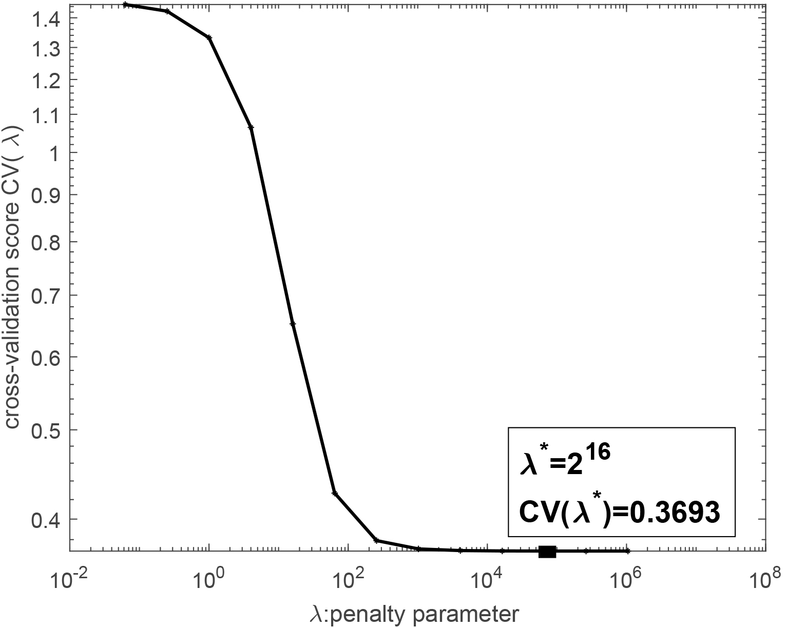
The relationship between the score of cross validation $CV(\lambda)$ and the penalty parameter $\lambda$ .

Figure 2.

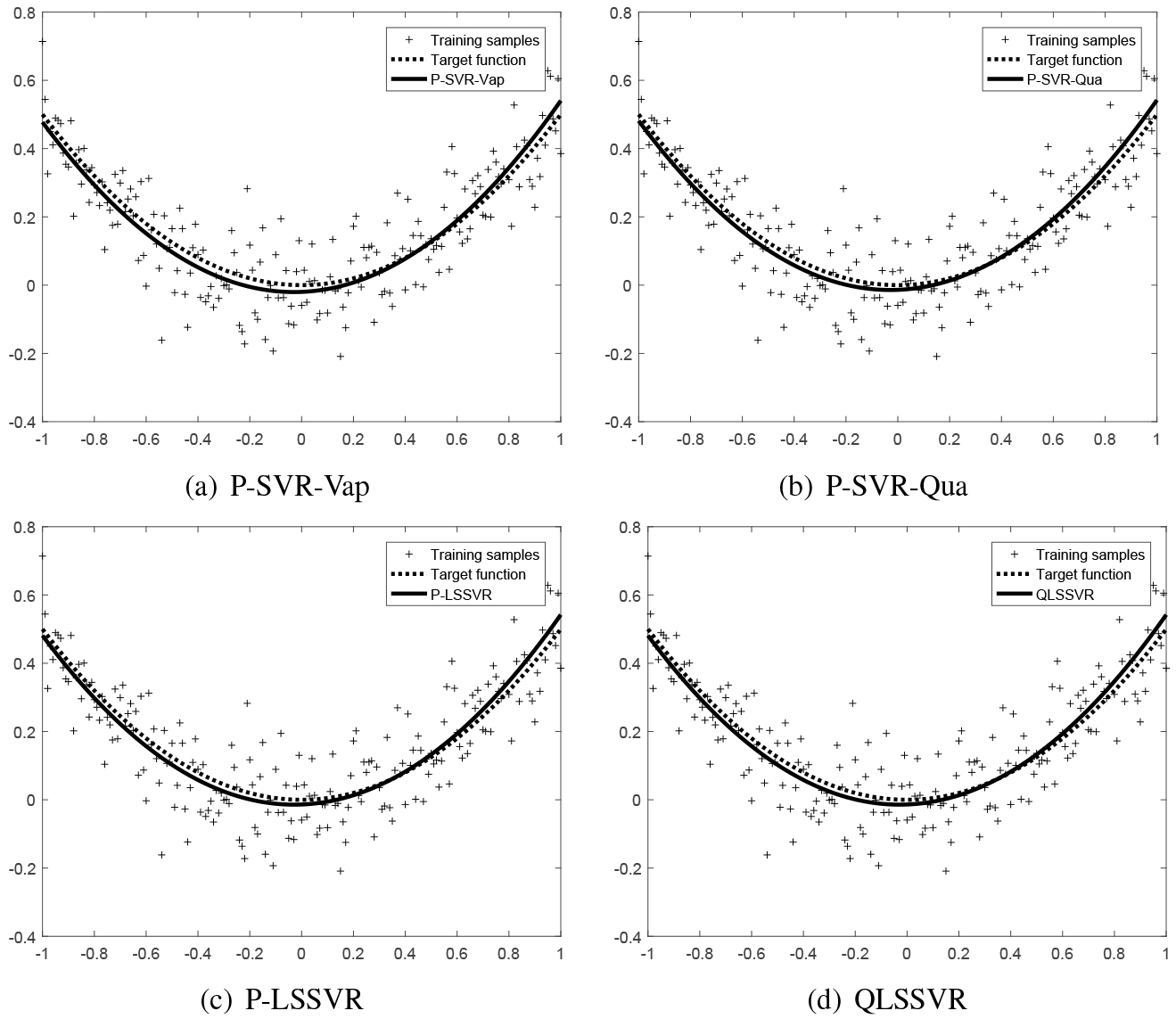
Comparing the results of P-SVR-Vap, P-SVR-Qua, P-LSSVR and QLSSVR.

In all the computations, the penalty parameters are selected from the grid-set of values $\{2^{i}|i=-4,-2,\cdots,20\}$ by cross validation. For comparison, we adopt the mean absolute error (MAE) and mean square error (MSE) to measure fitting error. We also calculate the sum squared error (SSE) and interpretable sum squared deviation of regression (SSR), sum squared deviation of testing samples (SST), and two ratio indexes from them to verify the fitting performance. One is that the smaller the value of SSE/SST is, the better the regression effect will be. The larger the value of SSR/SST is, the better the regression effect will be. The definitions of these evaluation criteria are given as

$\displaystyle\text{MAE}=\frac{1}{n}\sum_{i=1}^{n}\mid y_{i}-f(\bm{x_{i}})\mid,$ $\displaystyle\text{MSE}=\frac{1}{n}\sum_{i=1}^{n}(y_{i}-f(\bm{x_{i}}))^{2},$ $\displaystyle\text{SSE}=\sum_{i=1}^{n}(y_{i}-f(\bm{x_{i}}))^{2},$ $\displaystyle\text{SSR}=\sum_{i=1}^{n}(f(\bm{x_{i}})-\overline{y})^{2},$ $\displaystyle\text{SST}=\sum_{i=1}^{n}(y_{i}-\overline{y})^{2},$

where $n$ is the number of testing samples, $y_{i}$ is the real value of a input $\bm{x_{i}}$ and $f(\bm{x_{i}})$ is the predicted value of a input $\bm{x_{i}}$ , $\overline{y}$ is the means of $y_{1},y_{2},\cdots,y_{n}$ .

4.1 Synthetic datasets

4.1.1 Geometric interpretation

To visually reflect the performance of our proposed QLSSVR, we first implement it on synthetic datasets $y=0.5x^{2}+\xi$ function, where $x\in[-1,1]$ and $\xi\sim N(0,0.1)$ . Specifically, 201 points $\{(x_{i},y_{i})\}_{i=1}^{201}$ are sampled on the closed interval $[-1,1]$ and the output $y_{i}$ is added by the Gaussian noise with the mean $\mu=0$ and the variance $\sigma=0.1$ . The 201 points are randomly split into two parts, which 80% points are as the training set, and the rest of the points are as the test set.

To evaluate the performance of our proposed QLSSVR on the synthetic datasets, we define the following score of cross validation

$\displaystyle CV(\lambda)=\sum_{i=1}^{l}\left(\overline{y}_{i}-\left(\frac{1}{% 2}\overline{x}_{i}^{T}W_{\lambda}\overline{x}_{i}+b_{\lambda}^{T}\overline{x}_% {i}+c_{\lambda}\right)\right)^{2},$ (29)

where the point $(\overline{x}_{i},\overline{y}_{i})$ cames from the test set after randomly removing the training set, $W_{\lambda}=\text{mat}(w_{\lambda})$ , $b_{\lambda}$ and $c_{\lambda}$ are obtained by Eq. (11) on the training set and $l=\lfloor 20\%\times 201\rfloor$ . Figure 1 shows the relationship between cross validation score $CV(\lambda)$ and $\lambda$ , when $\lambda$ ranged from $2^{-4}$ to $2^{20}$ with the ratio 2. In fact, we can also see that, with the increase of $\lambda$ , the score of cross validation $CV(\lambda)$ gradually decreases, and then reaches a flat level. When $\lambda=2^{16}$ , the score $CV(\lambda)$ reaches the minimum 0.3693, that is, the optimal penalty parameter $\lambda^{*}$ is $2^{16}$ .

Next, we present the results of P-SVR-Vap, P-SVR-Qua, P-LSSVR, and our proposed QLSSVR on the synthetic datasets in Fig. 2 when the penalty parameter $\lambda^{*}$ is $2^{16}$ . It can be seen from Fig. 2 that our proposed QLSSVR has a similar fit to the other three methods with the quadratic polynomial kernel function, although our approach does not require the use of a kernel function.

Table 1

Comparing the CPU running times of different methods with the different data sizes $n$ and input dimensions $m$ (CPU time: sec.)

Data points	Methods	$m=$ 2	$m=$ 4	$m=$ 8	$m=$ 16	$m=$ 24	$m=$ 32
$n=$ 200	P-SVR-Vap	1.9269	1.7800	1.8691	1.6309	1.0150	1.2839
	P-SVR-Qua	1.2288	1.1988	1.1570	1.1473	0.9679	1.1364
	P-LSSVR	1.1063	1.0994	1.1178	1.1198	1.0435	1.1615
	QLSSVR	0.1304	0.1373	0.1345	0.2791	0.6321	2.4602
$n=$ 400	P-SVR-Vap	14.1307	9.8510	7.5796	7.3327	6.3389	4.1023
	P-SVR-Qua	4.4078	4.2272	3.8165	3.8140	3.7799	3.7343
	P-LSSVR	3.6186	3.5730	3.6509	3.6278	3.9136	3.6326
	QLSSVR	0.1117	0.1078	0.1255	0.3885	1.1698	3.0897
$n=$ 600	P-SVR-Vap	27.3528	33.0550	20.5308	17.7407	16.8083	13.1874
	P-SVR-Qua	9.6201	8.7496	8.2190	8.3290	8.7816	8.3433
	P-LSSVR	8.1818	8.0694	8.1142	8.2005	8.6140	8.2459
	QLSSVR	0.1424	0.1354	0.2019	0.5704	1.5748	4.5991
$n=$ 800	P-SVR-Vap	99.6186	60.6332	39.7413	35.5498	36.7134	30.2127
	P-SVR-Qua	19.1237	16.2576	14.7880	14.7339	14.7124	14.7524
	P-LSSVR	14.8736	14.4905	14.5642	14.5241	14.5201	14.9214
	QLSSVR	0.1914	0.1911	0.2369	0.7367	2.0562	5.9857
$n=$ 1000	P-SVR-Vap	185.2633	111.2788	85.2383	66.4834	79.5502	68.8742
	P-SVR-Qua	24.6751	22.8673	26.6687	26.4496	26.2827	25.6121
	P-LSSVR	22.2680	22.4359	22.5679	24.8718	25.1144	24.7836
	QLSSVR	0.2088	0.2129	0.3070	1.1921	3.3127	11.8244

4.1.2 Comparing the CPU time

To compare the computation time of our proposed QLSSVR with those of the standard SVR and LSSVR with quadratic polynomial kernel, we still reconstruct the synthetic datasets of different sizes with different dimensions for the quadratic function $y_{i}=0.5x_{i}^{2}+\xi_{i}$ , where $x_{i}\in R^{m}$ , obeys standard uniform distribution, $\xi_{i}\in R$ , $i=1,2,\dots,n$ , obeys normal distribution with the mean $\mu=0$ and the variance $\sigma=0.1$ . Specifically, the dimension of the input $m$ is from the set $\{2,4,8,16,24,32\}$ , and the number of the training points $n$ is from the set $\{200i|i=1,2,\cdots,5\}$ .

Table 1 shows the CPU time of P-SVR-Vap, P-SVR-Qua, P-LSSVR and our proposed QLSSVR are performed on the synthetic datasets with the different data sizes $n$ and input dimensions $m$ . The best performing results are marked in bold font. From Table 1, it can be seen that the performance of our proposed QLSSVR is optimal because it is kernel-free. And it is obvious that the CPU time of P-SVR-Vap are seriously affected by the sizes of the training points.

Figure 3.

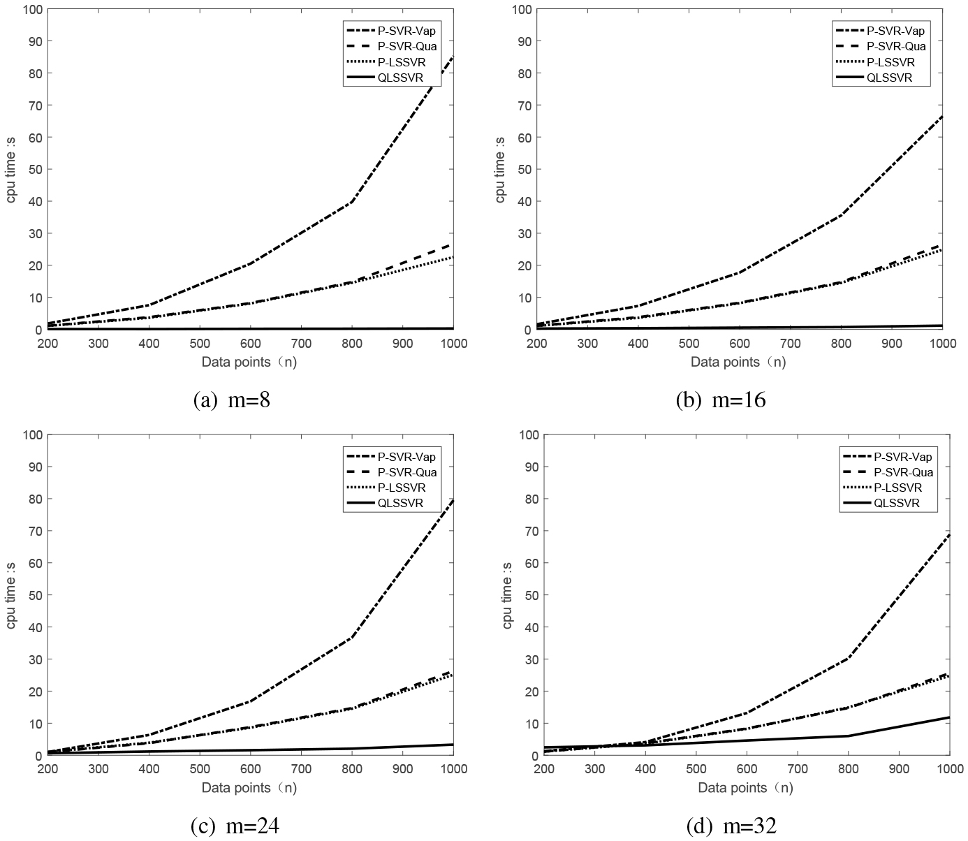
CPU running times of the different methods with the different data sizes when $m=$ 8, 16, 24 and 32.

In addition, we also show the line charts of the CPU running times of different methods with the different data sizes $n$ and input dimensions $m$ in Figs 3 and 4. Specifically, in Fig. 3, we present the line charts of the change between the CPU time and the number of the training points, where the input dimension $m=$ 8, 16, 24 and 32. It can be seen that the CPU time of our proposed QLSSVR increases slowly with the increase of the input dimension $m$ , though. The CPU time of the other three approaches increase rapidly, especially, the standard SVR with the quadratic polynomial kernel.

Figure 4.

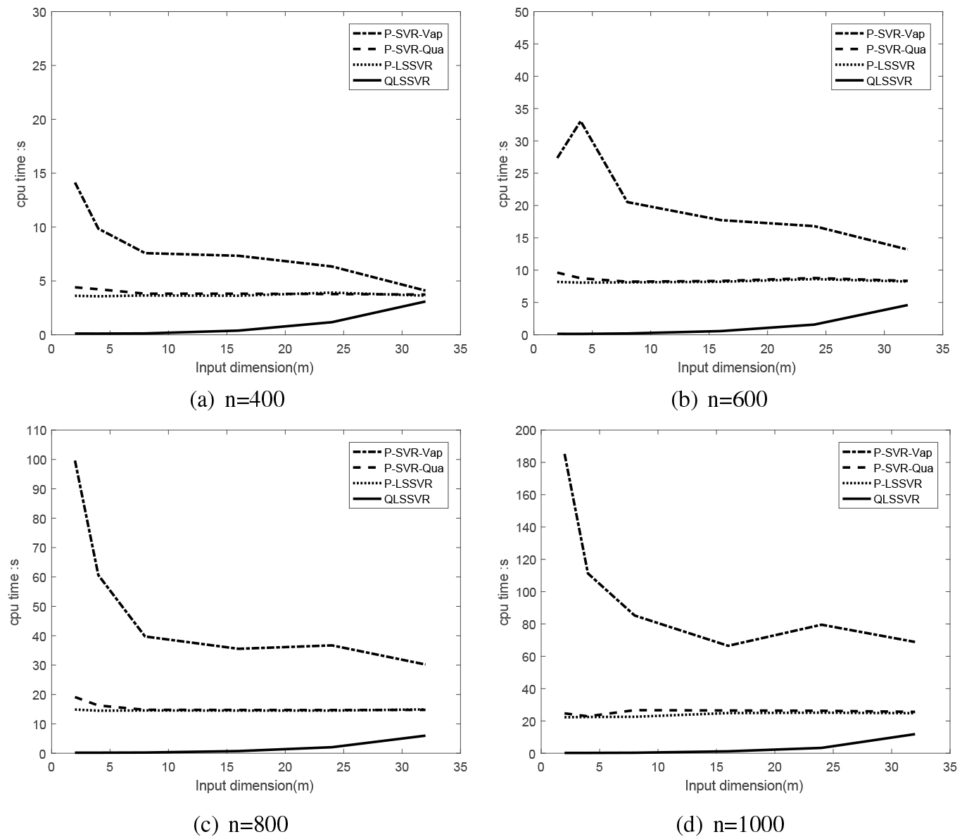
The CPU time of the different methods with the different dimensions of the inputs when $n=$ 400, 600, 800 and 1000.

In Fig. 4, we show the line charts of the change between the CPU time and the dimensions of the inputs, where the number of the training points $n=$ 400, 600, 800 and 1000. Although, when the dimension of the inputs increases, the CPU time of our proposed QLSSVR will increase slightly, but overall it is less time spent than the other three approaches. Furthermore, when the dimension of the inputs $m$ is less than 20, the CPU time of our proposed QLSSVR can always be kept below 1 second.

Table 2

Comparison of MAE and MSE of different approaches for the different input dimensions $m$ and different data sizes $n$

Data points	Methods	$m=$ 2	$m=$ 4	$m=$ 8	$m=$ 16	$m=$ 24	$m=$ 32
$n=$ 200	P-SVR-Vap	0.080/0.010	0.084/0.011	0.061/0.008	0.026/0.005	3.0e-9/1.4e-17	5.6e-10/5.5e-19
	P-SVR-Qua	0.092/0.014	0.082/0.010	0.062/0.006	0.037/0.002	5.5e-8/5.4e-15	2.0e-8/6.4e-16
	P-LSSVR	0.080/0.009	0.071/0.008	0.066/0.007	0.043/0.003	1.3e-7/2.8e-14	4.0e-8/3.2e-15
	QLSSVR	0.073/0.008	0.075/0.009	0.072/0.008	0.040/0.003	8.3e-6/1.8e-10	2.8e-6/1.4e-11
$n=$ 400	P-SVR-Vap	0.080/0.010	0.077/0.009	0.072/0.009	0.054/0.008	0.020/0.003	2.8e-6/1.2e-11
	P-SVR-Qua	0.077/0.009	0.080/0.010	0.077/0.009	0.063/0.006	0.033/0.002	5.6e-8/5.2e-15
	P-LSSVR	0.078/0.010	0.084/0.011	0.079/0.010	0.069/0.007	0.037/0.002	1.4e-7/3.4e-14
	QLSSVR	0.076/0.009	0.075/0.009	0.073/0.009	0.062/0.006	0.036/0.002	1.5e-5/3.8e-10
$n=$ 600	P-SVR-Vap	0.077/0.009	0.081/0.011	0.077/0.010	0.061/0.008	0.047/0.007	0.018/0.005
	P-SVR-Qua	0.077/0.009	0.077/0.010	0.074/0.009	0.066/0.007	0.049/0.004	0.021/0.001
	P-LSSVR	0.078/0.009	0.078/0.010	0.077/0.009	0.070/0.008	0.053/0.004	0.024/0.001
	QLSSVR	0.079/0.010	0.081/0.010	0.077/0.009	0.070/0.008	0.053/0.005	0.026/0.001
$n=$ 800	P-SVR-Vap	0.082/0.010	0.078/0.010	0.080/0.011	0.069/0.009	0.052/0.008	0.033/0.006
	P-SVR-Qua	0.078/0.009	0.078/0.010	0.078/0.010	0.069/0.008	0.061/0.006	0.043/0.003
	P-LSSVR	0.076/0.009	0.081/0.011	0.079/0.010	0.072/0.008	0.060/0.006	0.043/0.003
	QLSSVR	0.077/0.009	0.081/0.010	0.079/0.010	0.072/0.008	0.059/0.005	0.042/0.003
$n=$ 1000	P-SVR-Vap	0.079/0.010	0.078/0.010	0.075/0.010	0.067/0.009	0.060/0.009	0.042/0.006
	P-SVR-Qua	0.082/0.011	0.084/0.011	0.081/0.010	0.071/0.008	0.067/0.007	0.052/0.004
	P-LSSVR	0.085/0.011	0.087/0.012	0.076/0.009	0.074/0.009	0.065/0.007	0.054/0.005
	QLSSVR	0.078/0.009	0.076/0.009	0.080/0.010	0.077/0.009	0.065/0.007	0.052/0.004

Tables 2 and 3 show the comparison of the MAE, MSE, $D_{1}=\textit{SSE/SST}$ and $D_{2}=\textit{SSR/SST}$ of the four approaches for the different input dimensions $m$ and different data sizes $n$ . Combining Tables 1–3, it can be clearly seen that our proposed QLSSVR not only has better values of regression criterions at different dataset scales, but also have the least CPU time.

Table 3

Comparison of $D_{1}=\textit{SSE/SST}$ and $D_{2}=\textit{SSR/SST}$ of different approaches for the different input dimensions $m$ and different data sizes $n$

Data points	Methods	$m=$ 2	$m=$ 4	$m=$ 8	$m=$ 16	$m=$ 24	$m=$ 32
$n=$ 200	P-SVR-Vap	0.195/0.802	0.133/0.861	0.034/1.004	0.015/0.998	3.4e-17/1.00	6.8e-19/1.00
	P-SVR-Qua	0.229/0.803	0.102/0.898	0.030/0.970	0.006/0.994	9.7e-15/1.00	9.8e-16/1.00
	P-LSSVR	0.186/0.814	0.078/0.923	0.046/0.955	0.009/0.992	5.0e-14/1.00	4.3e-15/1.00
	QLSSVR	0.176/0.824	0.090/0.910	0.039/0.961	0.006/0.994	3.0e-10/1.00	1.9e-11/1.00
$n=$ 400	P-SVR-Vap	0.175/0.798	0.102/0.894	0.050/0.925	0.021/0.986	0.005/0.994	1.6e-11/1.00
	P-SVR-Qua	0.152/0.848	0.093/0.907	0.050/0.950	0.018/0.982	0.003/0.997	7.2e-15/1.00
	P-LSSVR	0.208/0.792	0.097/0.903	0.049/0.951	0.019/0.981	0.004/0.996	4.4e-14/1.00
	QLSSVR	0.183/0.817	0.080/0.921	0.051/0.949	0.013/0.987	0.004/0.996	5.0e-10/1.00
$n=$ 600	P-SVR-Vap	0.174/0.867	0.101/0.913	0.060/0.947	0.023/0.978	0.014/0.996	0.006/0.999
	P-SVR-Qua	0.169/0.831	0.110/0.890	0.053/0.947	0.020/0.980	0.007/0.993	0.001/0.999
	P-LSSVR	0.167/0.833	0.098/0.902	0.052/0.948	0.021/0.979	0.008/0.992	0.001/0.999
	QLSSVR	0.193/0.807	0.108/0.892	0.052/0.948	0.018/0.982	0.008/0.992	0.002/0.998
$n=$ 800	P-SVR-Vap	0.180/0.823	0.096/0.908	0.057/0.951	0.025/0.974	0.015/0.989	0.008/0.999
	P-SVR-Qua	0.172/0.828	0.102/0.898	0.053/0.947	0.021/0.979	0.010/0.990	0.004/0.996
	P-LSSVR	0.179/0.821	0.111/0.889	0.056/0.944	0.021/0.979	0.010/0.990	0.004/0.996
	QLSSVR	0.165/0.835	0.100/0.900	0.052/0.948	0.021/0.979	0.010/0.991	0.004/0.996
$n=$ 1000	P-SVR-Vap	0.189/0.825	0.102/0.889	0.048/0.940	0.024/0.958	0.016/0.988	0.009/0.994
	P-SVR-Qua	0.189/0.753	0.111/0.829	0.062/0.938	0.023/0.977	0.013/0.987	0.006/0.994
	P-LSSVR	0.208/0.708	0.115/0.818	0.053/0.947	0.024/0.976	0.013/0.988	0.006/0.994
	QLSSVR	0.169/0.831	0.097/0.903	0.055/0.945	0.025/0.975	0.012/0.988	0.006/0.995

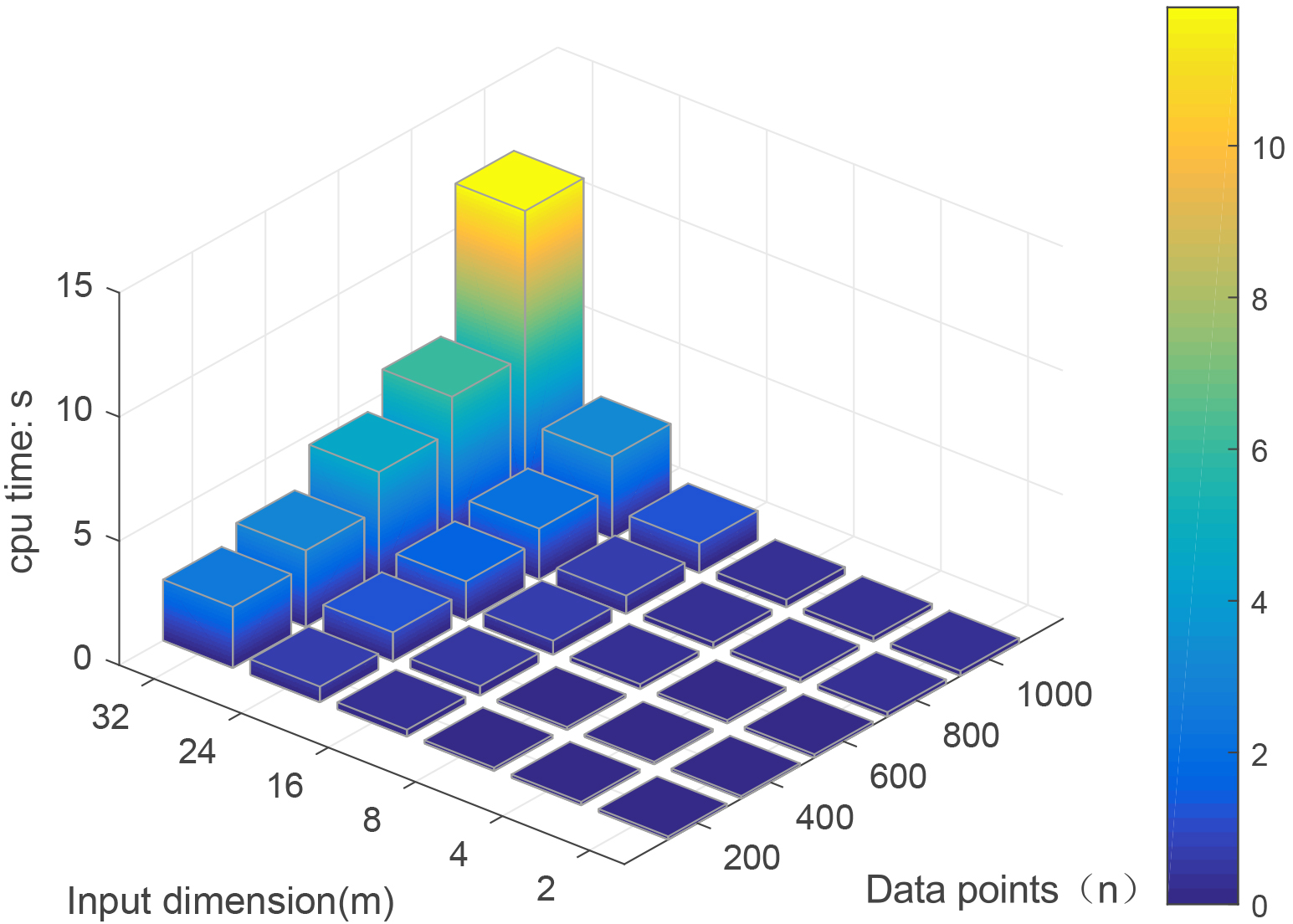
Finally, to show the performance of our proposed QLSSVR more intuitively. We present a three-dimensional color gradient histogram with the input dimension, data scale, and CPU time of QLSSVR in Fig. 5. It can be seen that the CPU time of our proposed QLSSVR are less than 15 seconds for all the scales of datasets, although the time obviously increases when the dimension of the inputs is over 16.

4.2 Benchmark datasets

In this section, we show the comparison on UCI benchmark datasets, i.e., we have tested the efficacy of the algorithms on eleven benchmark datasets which includes Concrete slump, Yacht, Energy_Heating, Energy_Cooling, House, Real estate valuation, QSAR fish toxicity, AirfoilSelf_Noise, Skill craft, MG and Space_ga. Table 4 shows the detail of the eleven benchmark datasets. In particular, there are missing values in skill craft data set. We use the mean value of the attribute to complete. All the datasets are normalized to between 0 and 1. In fact, according to the number of the training points, the eleven datasets are divided into two groups based on the numbers of training points, the first six datasets as one group, the rest as another group. To select the optimal parameter, we use 10-fold cross-validation at the first six benchmark datasets. We use 3-fold cross-validation at the rest of the benchmark datasets because their numbers of training points are over 1000. Notably, due to the excessive amount of training points in SkillCraft master and Space_ga, we have increased the step size of the search grid to save time.

Table 4
Detailed information about benchmark data sets

Data sets	#samples	#attributes	Missing values
Concrete slump	103	7	No
Yacht	308	6	No
Energy_Heating	768	8	N0
Energy_Cooling	768	8	No
House	506	13	No
Real estate valuation	414	6	No
QSAR fish toxicity	908	6	No
AirfoilSelf_Noise	1503	6	No
Skill Craft	3395	18	Yes
Mg	1385	6	No
Space_ga	3107	6	No

#denotes the number of.

Figure 5.

Three dimensional color gradient histogram with input dimension, data scale and CPU time of QLSSVR.

Table 5

Comparision the overall performance of QSLSSVR with some advanced methods on the first group of benchmark data sets (Mean/Std)

Data sets	Methods	MAE	MSE	$D_{1}=\frac{\textit{SSE}}{\textit{SST}}$	$D_{2}=\frac{\textit{SSR}}{\textit{SST}}$	Time1 (:s)	Time2 (:s)
Concrete slump	L-SVR-Vap	0.0059/0.0003	0.0041/9.8e-6	0.1252/0.0147	0.8809/0.0213	35.64	3.95
	L-SVR-Qua	0.0063/0.0004	0.0041/7.7e-6	0.1247/0.0108	0.8582/0.0281	28.37	3.62
	L-LSSVR	0.0062/0.0004	0.0041/8.0e-6	0.1262/0.0116	0.8635/0.0167	27.90	2.62
	QLSSVR	0.0010/9.8e-6	0.0003/3.2e-8	0.0089/5.0e-5	0.9759/0.0046	18.42	2.13
	P-SVR-Vap	0.0008/6.1e-6	0.0002/5.3e-8	0.0074/2.6e-5	0.9874/0.0033	28.13	6.61
	P-SVR-Qua	0.0010/9.8e-6	0.0003/3.2e-8	0.0090/5.2e-5	0.9826/0.0055	22.84	3.82
	P-LSSVR	0.0010/9.0e-6	0.0003/3.2e-8	0.0091/5.3e-5	0.9799/0.0058	19.45	4.42
Yacht	L-SVR-Vap	0.0084/0.0007	0.0283/0.0001	0.4774/0.0020	0.2215/0.0060	198.56	13.19
	L-SVR-Qua	0.0099/0.0010	0.0205/7.1e-5	0.3515/0.0027	0.6308/0.0148	148.10	10.75
	L-LSSVR	0.0088/0.0008	0.0204/7.0e-5	0.3500/0.0020	0.6106/0.0166	78.61	6.05
	QLSSVR	0.0066/0.0004	0.0050/4.6e-6	0.0889/0.0009	0.9496/0.0250	9.07	0.69
	P-SVR-Vap	0.0045/0.0002	0.0067/1.4e-5	0.1117/0.0008	0.7053/0.0151	197.10	15.19
	P-SVR-Qua	0.0061/0.0004	0.0049/4.3e-6	0.0869/0.0007	0.9486/0.0224	85.88	6.67
	P-LSSVR	0.0058/0.0003	0.0049/4.3e-6	0.0862/0.0007	0.9399/0.0215	81.90	6.37
Energy heating	L-SVR-Vap	0.0052/0.0003	0.0065/1.8e-6	0.0885/0.0005	0.8833/0.0012	1681.31	123.64
	L-SVR-Qua	0.0053/0.0003	0.0062/1.2e-6	0.0853/0.0003	0.8958/0.0015	1080.26	80.58
	L-LSSVR	0.0053/0.0003	0.0062/1.2e-6	0.0852/0.0003	0.8920/0.0016	477.88	36.92
	QLSSVR	0.0020/4.1e-5	0.0008/1.7e-8	0.0106/5.6e-6	0.9875/0.0012	17.94	1.31
	P-SVR-Vap	0.0017/2.8e-5	0.0004/1.5e-8	0.0059/3.4e-6	1.0049/0.0002	1824.72	188.96
	P-SVR-Qua	0.0018/3.1e-5	0.0006/1.2e-8	0.0079/3.1e-6	0.9905/0.0002	535.06	41.94
	P-LSSVR	0.0019/3.6e-5	0.0008/1.8e-8	0.0104/4.7e-6	0.9870/0.0003	498.50	38.97
Energy cooling	L-SVR-Vap	0.0052/0.0003	0.0076/3.7e-6	0.1173/0.0006	0.8978/0.0058	1820.84	132.54
	L-SVR-Qua	0.0053/0.0003	0.0074/3.5e-6	0.1143/0.0005	0.8891/0.0038	1083.65	81.20
	L-LSSVR	0.0053/0.0003	0.0074/3.4e-6	0.1141/0.0005	0.8871/0.0036	481.15	36.93
	QLSSVR	0.0037/0.0001	0.0027/8.1e-8	0.0426/6.4e-5	0.9565/0.0024	17.60	1.32
	P-SVR-Vap	0.0029/0.0001	0.0028/2.4e-7	0.0439/3.4e-5	0.9610/0.0107	2082.07	202.98
	P-SVR-Qua	0.0033/0.0001	0.0023/1.1e-7	0.0357/2.3e-5	0.9673/0.0025	539.83	42.28
	P-LSSVR	0.0038/0.0001	0.0027/1.0e-7	0.0411/2.6e-5	0.9634/0.0026	498.40	38.36
House	L-SVR-Vap	0.0082/0.0007	0.0119/4.2e-5	0.2868/0.0107	0.6846/0.0255	1298.29	88.52
	L-SVR-Qua	0.0083/0.0007	0.0115/3.0e-5	0.2799/0.0075	0.7343/0.0201	691.45	57.20
	L-LSSVR	0.0083/0.0007	0.0115/3.0e-5	0.2809/0.0077	0.7498/0.0215	360.41	37.11
	QLSSVR	0.0053/0.0003	0.0050/2.6e-6	0.1342/0.0049	0.9036/0.0045	35.39	4.15
	P-SVR-Vap	0.0060/0.0004	0.0055/1.2e-5	0.1368/0.0045	0.8847/0.0074	1326.96	124.62
	P-SVR-Qua	0.0053/0.0003	0.0048/2.6e-6	0.1298/0.0037	0.9229/0.0056	425.75	37.00
	P-LSSVR	0.0053/0.0003	0.0049/2.6e-6	0.1306/0.0038	0.9301/0.0073	377.10	36.88
Real estate valuation	L-SVR-Vap	0.0061/0.0004	0.0065/2.1e-5	0.4173/0.0208	0.6116/0.0247	844.40	44.57
	L-SVR-Qua	0.0062/0.0004	0.0066/2.0e-5	0.4283/0.0213	0.6154/0.0274	1061.90	46.13
	L-LSSVR	0.0062/0.0004	0.0066/2.0e-5	0.4285/0.0212	0.6057/0.0272	639.68	50.73
	QLSSVR	0.0051/0.0003	0.0051/1.6e-5	0.3237/0.0208	0.7378/0.0322	40.46	2.70
	P-SVR-Vap	0.0053/0.0003	0.0052/1.6e-5	0.3320/0.0221	0.7262/0.0286	2435.33	163.55
	P-SVR-Qua	0.0052/0.0003	0.0051/1.7e-5	0.3216/0.0211	0.7260/0.0280	550.69	58.81
	P-LSSVR	0.0052/0.0003	0.0051/1.7e-5	0.3223/0.0210	0.7170/0.0300	663.44	34.05

Table 5 shows the comparison results for the first six benchmark datasets, while Table 6 shows the comparison results for the other five benchmark datasets. For each dataset, we all compare the result of our proposed QLSSVR with those of the six approaches mentioned earlier: L-SVR-Vap, L-SVR-Qua, L-LSSVR, P-SVR-Vap, and P-SVR-Qua. And we list the following criteria: MAE, MSE, $D_{1}=\textit{SSE/SST}$ , $D_{2}=\textit{SSR/SST}$ , Time1 and Time2 for each approach, where Time1 is the CPU time for choosing optimal parameter by $k$ -fold cross-validation and Time2 is the CPU time for the final test. All the results are repeated $k$ times independently, where $k=10$ and 3. The best results are represented by a boldface.

From Tables 5 and 6, the QLSSVR derives the best criterion for almost all the datasets when compared to SVR and LSSVR with linear kernel. Compared to SVR and LSSVR with quadratic polynomial kernel, the QLSSVR performs similarly in case of benchmark datasets. It is worth noting that the clearly shows the superiority of QLSSVR over the other approaches in terms of the CPU time.

Table 6

Comparing the overall performance of QLSSVR with some advanced methods on the second group of benchmark data sets (Mean/Std)

Data sets	Methods	MAE	MSE	$D_{1}=\frac{\textit{SSE}}{\textit{SST}}$	$D_{2}=\frac{\textit{SSR}}{\textit{SST}}$	Time1 (:s)	Time2 (:s)
QSAR fish toxicity	L-SVR-Vap	0.0240/0.0017	0.0101/1.0e-6	0.4357/0.0004	0.5537/3.4e-5	1588.89	67.62
	L-SVR-Qua	0.0239/0.0017	0.0101/1.0e-6	0.4355/0.0005	0.5387/0.0013	560.41	27.52
	L-LSSVR	0.0240/0.0017	0.0101/9.9e-7	0.4363/0.0004	0.5511/0.0023	235.71	25.52
	QLSSVR	0.0230/0.0016	0.0096/3.1e-7	0.4133/1.2e-5	0.6197/0.0011	12.99	1.48
	P-SVR-Vap	0.0232/0.0016	0.0097/7.7e-7	0.4191/0.0007	0.6992/0.0008	960.63	63.91
	P-SVR-Qua	0.0233/0.0016	0.0096/3.7e-7	0.4148/0.0001	0.6143/0.0012	266.72	22.81
	P-LSSVR	0.0230/0.0016	0.0096/3.6e-7	0.4142/0.0001	0.6212/0.001	297.58	21.83
AirfoilSelf noise	L-SVR-Vap	0.0331/0.0033	0.0166/1.6e-6	0.5001/0.0059	0.5652/0.0058	3661.93	140.77
	L-SVR-Qua	0.0334/0.0034	0.0165/1.1e-6	0.4954/0.0043	0.4946/0.0012	2356.87	196.56
	L-LSSVR	0.0334/0.0034	0.0165/1.1e-6	0.4950/0.0042	0.4739/0.0003	1448.30	134.05
	QLSSVR	0.0292/0.0025	0.0124/1.6e-6	0.3735/0.0031	0.6539/0.0056	18.35	1.90
	P-SVR-Vap	0.0287/0.0025	0.0132/2.5e-6	0.3981/0.0054	0.7556/0.0010	5073.81	371.67
	P-SVR-Qua	0.0292/0.0026	0.0124/1.6e-6	0.3734/0.0031	0.6558/0.0055	1714.50	93.61
	P-LSSVR	0.0292/0.0026	0.0124/1.6e-6	0.3733/0.0031	0.6551/0.0055	1575.95	142.65
Skill craft	L-SVR-Vap	0.0130/0.0005	0.0047/3.8e-8	0.6329/0.0040	0.2702/0.0011	13494.80	1742.20
	L-SVR-Qua	0.0125/0.0005	0.0045/6.3e-8	0.6191/0.0056	0.3548/0.0049	2706.63	787.84
	L-LSSVR	0.0125/0.0005	0.0045/8.5e-8	0.6183/0.0062	0.3986/0.0039	1035.21	298.66
	QLSSVR	0.0124/0.0005	0.0042/2.0e-7	0.5646/0.0029	0.4860/0.0228	40.83	14.66
	P-SVR-Vap	0.0106/0.0003	0.0045/2.1e-7	0.6087/0.0011	0.3951/0.0095	8125.40	2517.60
	P-SVR-Qua	0.0125/0.0005	0.0041/2.0e-7	0.5601/0.0023	0.5006/0.0293	910.31	312.88
	P-LSSVR	0.0133/0.0005	0.0042/2.1e-7	0.5617/0.0021	0.5398/0.0068	2318.94	487.09
Mg	L-SVR-Vap	0.0403/0.0049	0.0219/7.6e-7	0.4287/0.0007	0.5745/0.0024	1645.82	116.88
	L-SVR-Qua	0.0410/0.0050	0.0214/1.8e-6	0.4185/0.0013	0.5776/0.0008	950.17	111.32
	L-LSSVR	0.0410/0.0050	0.0214/1.9e-6	0.4187/0.0013	0.5687/0.0003	642.75	54.54
	QLSSVR	0.0353/0.0037	0.0169/2.6e-7	0.3315/0.0003	0.6875/0.0012	20.11	1.67
	P-SVR-Vap	0.0356/0.0038	0.0179/9.0e-7	0.3499/0.0007	0.7113/0.0011	3648.55	299.22
	P-SVR-Qua	0.0353/0.0037	0.0169/2.7e-7	0.3316/0.0003	0.6861/0.0012	846.02	91.69
	P-LSSVR	0.0353/0.0037	0.0169/2.6e-7	0.3317/0.0003	0.6900/0.0012	1109.08	80.20
Space_ga	L-SVR-Vap	0.0105/0.0003	0.0017/3.7e-8	0.4234/0.0002	0.6057/0.0041	8156.68	2064.76
	L-SVR-Qua	0.0105/0.0003	0.0017/3.5e-8	0.4217/0.0002	0.5667/0.0017	6522.02	2106.80
	L-LSSVR	0.0105/0.0003	0.0017/3.4e-8	0.4223/0.0002	0.5524/0.0004	530.52	134.68
	QLSSVR	0.0090/0.0002	0.0013/1.3e-8	0.3307/0.0008	0.6633/0.0021	3.27	0.66
	P-SVR-Vap	0.0088/0.0002	0.0013/1.2e-8	0.3379/0.0016	0.6954/0.0063	20654.03	2285.5
	P-SVR-Qua	0.0090/0.0002	0.0013/1.4e-8	0.3336/0.0009	0.6659/0.0024	857.54	242.51
	P-LSSVR	0.0090/0.0002	0.0013/1.7e-8	0.3354/0.0007	0.6529/0.0021	561.99	138.17

5. Conclusions

For a regression problem, we propose a new method called as quadratic hyper-surface kernel-free least squares support vector regression (QLSSVR). In this approach, the quadratic function is used as the regression function such that the kernel is free, which is the main advantage of our approach. And the constraints of the quadratic programming only contains equalities, which results in finding the solution by solving a set of linear equations instead of a convex quadratic programming problem. The performance of our proposed QLSSVR is checked with the synthetic datasets and 11 benchmark datasets from the machine learning repository. The numerical results illustrate that our approach has better performance than other existing regression approaches in terms of regression criterion and CPU time.

Footnotes

Acknowledgments

The authors would like to thank the anonymous referees and editor for their valuable suggestions and helpful comments, which greatly improved the content and presentation of the paper.

This work is supported by Xinjiang Provincial Natural Science Foundation of China (No. 2020D01C028), the Xinjiang Provincial University Research Foundation of China (No. XJEDU2018I002) and the National Natural Science Foundation of China (No. 12061071).

Conflict of interest

The authors declare that they have no conflict of interest.

References

Abe

, Fuzzy support vector machines for multilabel classification, Pattern Recognition 48(6) (2015), 2110–2117.

S.J.

et al., Least squares support vector machines, World Scientific, 2002.

Bai

Han

Chen

and Yu

, Quadratic kernel-free least squares support vector machine for target diseases classification, Journal of Combinatorial Optimization 30(4) (2015), 850–870.

Balasundaram

Gupta

and Kapil, Lagrangian support vector regression via unconstrained convex minimization, Neural Netw. 51 (Mar. 2014), 67–79.

Boser

B.E.

Guyon

I.M.

and Vapnik

V.N.

, A training algorithm for optimal margin classifiers, in: Proceedings of the Fifth Annual Workshop on Computational Learning Theory, ACM, 1992, pp. 144–152.

Burges

C.J.

, A tutorial on support vector machines for pattern recognition, Data Mining and Knowledge Discovery 2(2) (1998), 121–167.

Cai

Wang

and Fan

, A multiple-kernel lssvr method for separable nonlinear system identification, Journal of Control Theory and Applications 11(4) (2013), 651–655.

Cherkassky

and Mulier

, Learning from data: concepts, theory, and methods john wiley and sons, New York, 1998.

Cleveland

Grosse

and Shyu

, Local regression models. statistical models in s (chambers, jm and hastie, tj, eds), 309–376, Wadsworth & Brooks, Pacific Grove, 1991.

10.

Cortes

and Vapnik

, Support-vector networks, Machine Learning 20(3) (1995), 273–297.

11.

Cover

T.M.

, Geometrical and statistical properties of systems of linear inequalities with applications in pattern recognition, IEEE Transactions on Electronic Computers (3) (1965), 326–334.

12.

Crammer

and Singer

, On the algorithmic implementation of multiclass kernel-based vector machines, Journal of Machine Learning Research 2(Dec) (2001), 265–292.

13.

Dagher

, Quadratic kernel-free non-linear support vector machine, Journal of Global Optimization 41(1) (2008), 15–30.

14.

Drucker

Burges

C.J.

Kaufman

Smola

A.J.

and Vapnik

, Support vector regression machines, in: Advances in Neural Information Processing Systems, 1997, pp. 155–161.

15.

Fan

Huang

et al., Profile likelihood inferences on semiparametric varying-coefficient partially linear models, Bernoulli 11(6) (2005), 1031–1057.

16.

Fletcher

, Practical methods of optimization, John Wiley & Sons, 2013.

17.

Glielmo

Sollich

and De Vita

, Accurate interatomic force fields via machine learning with covariant kernels, Physical Review B 95(21) (2017), 214302.

18.

Hofmann

Schölkopf

and Smola

A.J.

, Kernel methods in machine learning, in: The Annals of Statistics, 2008, pp. 1171–1220.

19.

Izonin

Trostianchyn

Duriagina

Tkachenko

Tepla

and Lotoshynska

, The combined use of the wiener polynomial and svm for material classification task in medical implants production, Int. J. Intell. Syst. Appl. (IJISA) 10(9) (2018), 40–47.

20.

Karal

, Maximum likelihood optimal and robust support vector regression with lncosh loss function, Neural Networks 94 (2017), 1–12.

21.

Khemchandani

Goyal

and Chandra

, Twsvr: regression via twin support vector machine, Neural Networks 74 (2016), 14–21.

22.

Nguyen

T.D.

Nguyen

and Phung

, Approximation vector machines for large-scale online learning, The Journal of Machine Learning Research 18(1) (2017), 3962–4016.

23.

Huber

M.B.

Lancianese

S.L.

Nagarajan

M.B.

Ikpot

I.Z.

Lerner

A.L.

and Wismuller

, Prediction of biomechanical properties of trabecular bone in mr images with geometric features and support vector regression, IEEE Transactions on Biomedical Engineering 58(6) (June 2011), 1820–1826.

24.

Mahmoodian

and Ebrahimian

, Using support vector regression in gene selection and fuzzy rule generation for relapse time prediction of breast cancer, Biocybernetics and Biomedical Engineering 36(3) (2016), 466–472.

25.

Marquardt

D.W.

, An algorithm for least-squares estimation of nonlinear parameters, Journal of the Society for Industrial and Applied Mathematics 11(2) (1963), 431–441.

26.

Naumovich

V.V.

Vapnik

et al., Statistical learning theory, 1998.

27.

Nelder

J.A.

and Wedderburn

R.W.

, Generalized linear models, Journal of the Royal Statistical Society: Series A (General) 135(3) (1972), 370–384.

28.

Peng

, Tsvr: an efficient twin support vector machine for regression, Neural Networks 23(3) (2010), 365–372.

29.

Ping

M.M.

and Xia

Y.Z.

\epsilon

-kernel-free soft quadratic surface support vector regression, Submitted.

30.

Zhang

and Xie

, Short-term wind speed or power forecasting with heteroscedastic support vector regression, IEEE Transactions on Sustainable Energy 7 (11 2015), 1–9.

31.

Zhang

Xie

and Wan

, Noise model based ν-support vector regression with its application to short-term wind speed forecasting, Neural Networks 57 (Sept. 2014), 1–11.

32.

Schaback

and Wendland

, Kernel techniques: from machine learning to meshless methods, Acta Numerica 15 (2006), 543–639.

33.

Steinwart

, Sparseness of support vector machines, Journal of Machine Learning Research 4(Nov) (2003), 1071–1105.

34.

Suykens

J.A.

and Vandewalle

, Least squares support vector machine classifiers, Neural Processing Letters 9(3) (1999), 293–300.

35.

Vapnik

Golowich

S.E.

and Smola

A.J.

, Support vector method for function approximation, regression estimation and signal processing, in: Advances in Neural Information Processing Systems, 1997, pp. 281–287.

Quadratic hyper-surface kernel-free least squares support vector regression

Abstract

Keywords

1. Introduction

2. Related work

2.1 Linear fitting

2.2 Nonlinear fitting

4.1.1 Geometric interpretation

Table 4 Detailed information about benchmark data sets

Footnotes

Acknowledgments

Conflict of interest

References

Table 4
Detailed information about benchmark data sets