Predictive modelling of hospital readmission: Evaluation of different preprocessing techniques on machine learning classifiers

Abstract

Hospital readmission is a major cost for healthcare systems worldwide. If patients with a higher potential of readmission could be identified at the start, existing resources could be used more efficiently, and appropriate plans could be implemented to reduce the risk of readmission. Therefore, it is important to predict the right target patients. Medical data is usually noisy, incomplete, and inconsistent. Hence, before developing a prediction model, it is crucial to efficiently set up the predictive model so that improved predictive performance is achieved. The current study aims to analyse the impact of different preprocessing methods on the performance of different machine learning classifiers. The preprocessing applied by previous hospital readmission studies were compared, and the most common approaches highlighted such as missing value imputation, feature selection, data balancing, and feature scaling. The hyperparameters were selected using Bayesian optimisation. The different preprocessing pipelines were assessed using various performance metrics and computational costs. The results indicated that the preprocessing approaches helped improve the model’s prediction of hospital readmission.

Keywords

Hospital readmission machine learning predictive modelling preprocessing

1. Introduction

Hospital readmission or re-hospitalisation is defined as a patient’s admission to a hospital either to the same or different hospital after being discharged, within a certain period, typically thirty days [92]. Hospital readmission has major financial implications for the healthcare system in many countries. It is also a crucial issue in the United States (US) [42]. These financial implications include increased operating revenues per patient, increased operating expenses per patient, and increased healthcare resources such as beds, doctors, and overtime pay for the staff, as well as related treatments. In theory, readmission risk is determined 1) as a quality metric of the hospital and 2) to target the delivery of resources to high-risk patients [52]. According to Laudicella et al. [54], the Centre of Medicare and Medicaid Services (CMS) in the United States, The National Centre for Health Outcomes Development (NCHOO) in the United Kingdom, and the Australian Institute of Health and Welfare (AIHW) in Australia informs the public about hospital readmission rates to indicate healthcare quality. These quality metrics serve as a benchmark for hospital management – to improve healthcare quality by reducing readmission rates. At the same time, this metric helps patients select hospitals that offer better care. Following this development, the research community has started to establish models for predicting hospital readmission rates.

Conventionally, models that predict hospital readmission usually target three groups, namely all-cause readmission, certain population diseases, and specific patient attributes. Kansagara et al. [52] reviewed the risk prediction models for the first target group. The study described the models’ performance and assessed their suitability for clinical or administrative use. The study found that most readmission risk prediction models had poor discriminative performance but should be further improved. This result might be due to the complex nature and many inherent limitations of predicting readmission risk. Most of the models incorporated variables such as medical comorbidity and past utilisation, while a few studies considered variables associated with overall health and function, the severity of illness, and social determinants of health. Similarly, Zhao et al. [105] reviewed the risk factors that could be widely generalised for all causes of unplanned re-hospitalisation, regardless of the target population or location. The study found that comorbidity indices could be considered as highly generalisable risk factors while health insurance was country-specific. Besides, the study found that about 34 risk factors were not specific to any population or location.

Meanwhile, a detailed review of the second target group was also done with a focus on certain population disease risk prediction models rather than all diseases. Ross et al. [80] contributed an essential review of the readmission of patients with the most critical disease, i.e., heart failure (HF). The study also reviewed the characteristics of patients that would be readmitted because of heart failure. Additionally, predictive analytics was conducted via a statistical model. The study found that Logistic Regression and Cox proportional hazards regression were the most commonly used analytics models. Conversely, the patient-level characteristics considered for the population included sociodemographic attributes (age and sex), comorbid conditions (diabetes mellitus and hypertension), and HF severity attributes (systolic ejection fraction).

Elsewhere, Rao et al. [76] reviewed the re-hospitalisation of stroke patients. They concluded that the common causes of readmission in this population were recurrent stroke, infections, and cardiac conditions. Moreover, Ali et al. [4], in their review of readmission after a hip fracture, concluded that patient-related factors such as age, comorbidities, and functional status were stronger predictors than hospital-related factors. Recently, Smith et al. [84] reviewed the performance of models that predicted the readmission of patients with Acute Myocardial Infarction (AMI). The study found that up until the time of the review, the existing risk prediction for AMI readmission had modest discrimination ability with uncertain generalisability because of methodological limitations. Most models incorporated demographic, comorbidity, and utilisation metric variables.

The third target group involves specific patient attributes, focusing only on certain criteria of the patient. For example, Garcia-Perez et al. [37] conducted a systematic review focusing on elderly patients. The study highlighted the need to investigate this group further, especially specific characteristics such as prior utilisation, length of hospital stay, morbidity, and poor functional ability.

Recently, many studies have started to use machine learning (ML) to predict hospital readmission due to the powerful capability of ML. Studies in this field applied different objectives, target populations that are readmitted, threshold readmission lengths (either 30-day readmission or other durations), and machine learning preprocessing pipelines, and classification algorithms. For instance, Artetxe et al. [9] conducted a systematic review of methods for predicting hospital readmission risk. The study found that machine learning models had evolved in recent years – from 2010 until now – reaching its peak in 2015. Additionally, some studies, for example, Futoma et al. [36], Tong et al. [90], and Frizzell et al. [35], also compared the performance of different machine learning models. However, these studies mainly focused on comparing several machine learning classifiers, with not much focus on preprocessing methods. The most challenging task in machine learning is preprocessing. This phase also consumes the most time in the model development process.

This study established the following research aims:

•
To provide an overview of the most commonly used preprocessing techniques and machine learning models for predicting hospital readmission from 2010 to 2019.
•
To provide an in-depth analysis of the effect of different preprocessing pipelines on the overall performance of readmission risk predictive models.
•
To introduce Bayesian optimisation to tune machine learning hyperparameters, as the literature has shown that this method could improve the overall performance of machine learning predictive models.

Hence, this paper adds to the existing body of work in this field three-fold. First, the impact of preprocessing pipelines, based on predictive models outlined in [9], were analysed, starting from the year 2010. Additionally, some recent studies that were not included in the review paper [9] were also analysed. Second, this study presented an analysis of the impact of different preprocessing pipelines, including feature selection, missing value imputation, data balancing, feature scaling, and classification algorithms on the overall performance of readmission risk predictive models. To the best of the authors’ knowledge, this is the first study to assess the suitability of commonly used preprocessing pipelines with overall hospital readmission predictive models. Finally, an alternative approach to existing predictive methods was introduced; namely, a powerful hyperparameter optimisation technique called Bayesian optimisation. To date, this approach has not yet been actively explored in addressing the readmission problem. This paper assesses the overall performance of the model based on two measures: a) classification evaluation metrics and b) computational cost.

The remainder of this paper is organised as follows: Section 2 presents the related works, while Section 3 elucidates the methodology of the hospital readmission framework. This methodology is divided into feature selection, missing value imputation, class imbalance, feature scaling, classification algorithm, and hyperparameter optimisation. Section 4 discusses the experimental data, the evaluation metrics, and the results of the analysis. Section 5 discusses the results and Section 6 presents the conclusion to this study and recommendations for future works.
2. Related works

Predictive modelling using ML models in hospital readmission has evolved in recent years. Numerous studies in light of readmission application had focused on the performance of the classification model, in comparison to preprocessing methods. Data preprocessing is beneficial in many ways, especially to ease the process of predictive modelling. In ML classifications, one can improve the quality of data and ensure useful information before proceeding to the next task.

Missing value imputation is the first preprocessing technique highlighted in the readmission study which refers to a missing critical value of an important attribute in an instance. Many medical datasets in existing databases have test groups that are absent or with incomplete information. This scenario might be due to several factors such as the lack of time due to clinical routines or the patient’s inability to perform a test [60], as well as insufficient monitoring [26]. Every value in a medical record is crucial for an accurate diagnosis. Besides, [41] mentioned that missing values and instances are common when utilising a common digitalised database, such as the Electronic Medical Record (EMR). This situation emerges because of the data collection method employed, especially when different facilities and multiple systems are involved. Among the common missing value imputation methods used are complete case deletion (CC) analysis, single imputation using mean/median and mode imputation (MMI), and multiple imputations by chained equation (MICE).

Nijhawan et al. [70], Mortazavi et al. [69], Lin et al. [59], and Leary et al. [55] used CC deletion analysis for the readmission task, while Zolfaghar et al. [107], AbdelRahman et al. [1], Shadmi et al. [82], Agrawal et al. [2], Golas et al. [41] and Wang et al. [100] used MMI. Meanwhile, Tulloch et al. [91] and Hatipoglu et al. [46] used MICE for the same task. However, these studies did not explain why they used missing imputation. Hence, this current review further analyses and assesses these imputation approaches (i.e., CC, MMI, and MICE) to determine their suitability to prediction tasks.

Another preprocessing method involved in the readmission task is feature selection, which has been widely applied in data analytics as it enables the researcher to identify the most significant variables in a dataset. In the medical domain, feature selection identifies the key factors associated with a disease and its specific risk conditions. For instance, feature selection helps the researcher to select a compact subset of attributes that helps maximise discrimination capability while reducing model complexity and overfitting [78]. At the same time, feature selection helps increase model interpretability [50]. It is common for readmission studies that use filter methods to employ univariate analysis, see [45, 15, 101, 72, 70, 104, 28, 107, 93, 81, 34, 12, 53, 65, 59, 62, 16, 92, 88, 49, 33, 19, 89, 55, 22, 46]. Firstly, filter feature selection operates on the characteristics of the data; it evaluates attributes without a classification algorithm. Then, it ranks the characteristics accordingly to decide whether the data should be removed from or kept in the dataset. Under the filter feature selection approach, readmission studies have also used multivariate analysis [39, 27, 36], Mutual Information-based methods such as information based on the Gini index [47, 1, 25, 79], Minimum-Redundancy-Maximum-Relevance (mRMR) [50], and Kullback-Leibler divergence [41].

The second frequently used feature selection was from the wrapper-based method. In contrast to the filter model, which selects variables independent of any classifier, the wrapper method uses a specific classifier to evaluate the performance of selected attributes. Previous studies that have applied the wrapper technique, especially forward selection, backward elimination or stepwise selection, include van Walraven et al. [94], Lopez-Aguila et al. [61], Allen et al. [5], Wallmann et al. [97], Allison et al. [6], Morris et al. [68], Pereira et al. [74], Tulloch et al. [91], Vigod et al. [96], Kaur et al. [53], Mortazavi et al. [69], Dorajoo et al. [30], Agrawal et al. [2], Greenwald et al. [43], Brauer et al. [17], Leary et al. [55], and Lim et al. [58].

Besides missing value imputation and feature selection, handling data imbalance is an acknowledged problem in hospital readmission as reported by Artetxe et al. [9]. Data balancing is applied to correct a class imbalance, which occurs when the number of instances, especially the target class (i.e. patient readmitted) is relatively very small compared to the other class [60]. Hospital readmission prediction involves a high class imbalance, resulting in a predictive model that is biased towards predicting the negative class (not readmitted) [51]. Of all the studies that had applied data balancing, about 70% used the resampling strategy [47, 98, 106, 69, 50, 44], 20% used the cost-sensitive strategy [69, 99] and the remaining used the ensemble strategy [92].

Apart from the commonly utilised preprocessing techniques mentioned above, the feature scaling approach is also crucial especially when the numerical values display wide variation. Only two studies have stated the use of feature scaling, wherein the related methods are normalisation [44] and standardisation [41]. Multiple studies pertaining to hospital readmission had adopted the preprocessing approach as part of their predictive modelling framework. As such, this study focused on the performance of classifier, while the impact of the different preprocessing methods is not discussed. The framework of hospital readmission is discussed in the next section, along with the detailed explanation of each preprocessing technique employed in this study.

Figure 1.

The overall framework for predicting hospital readmission.

3. Methodology

The overall framework for the selection of hospital readmission preprocessing methods and Machine Learning modelling is shown in Fig. 1. This figure provides an overview of the preprocessing approaches and machine learning classifiers used in previous hospital readmission predictive studies. The initial task starts with cleaning the collected data. Then, the subjects for the study, which are inpatient admission records, are identified. Since the task requires examining patients that could be readmitted in the future, patients that have died were removed. In this early phase, the most suitable study variables and the most appropriate data cleaning processes were determined based on proper domain insight and data familiarity. With reference to past studies concerning readmission and domain knowledge, only features potentially associated with hospital readmissions were retained.

3.1 Preprocessing pipeline

Before conducting any predictive analysis, it is important to ensure that a good dataset is chosen. In other words, the dataset must be clean and complete. The dataset for this study was denoted as $D$ . In any analysis, it is almost impossible to find a clean dataset because the data collection process is prone to human error. Hence, preprocessing is an essential step that must be applied for any predictive modelling task. However, in some cases, different preprocessing methods also cause a butterfly effect on the predictive model. Therefore, the most appropriate preprocessing method must be selected to ensure the model achieves good performance, and, therefore, yields good results. At the same time, the model can provide a correct overview of the problem at hand. Based on the extensive literature review of related studies [9], and with the help from domain experts, the most appropriate preprocessing methods were selected to ensure that the model yields exceptional performance. In this paper, the main focus was on missing value imputation, feature selection, data balancing, and feature scaling. These preprocessing methods are described in more detail in the next following subsection.

3.1.1 Missing value imputation

From the current investigation on the readmission problem, surprisingly, only about 20% of the studies reported using missing value imputation for preprocessing. Among the common missing value imputation methods used are complete case deletion (CC) analysis, single imputation using mean/median and mode imputation (MMI), and multiple imputations by chained equation (MICE). In most situations, simple techniques such as mean imputation, CC analysis, and missing-indicator methods were commonly used due to their ease of implementation. However, these simple techniques lead to biased results [29]. Besides, CC is generally not recommended because it leads to poor prediction and substantial bias [8] although it has been used widely because of its simplicity. The CC analysis, or also known as case-wise or list-wise deletion, removes all rows that have lost information while missing-indicator methods replace missing values with new dummy variables. On the other hand, MMI is one of the most commonly used methods for tackling many problems, including readmission tasks. This method simply replaces missing data in a numerical attribute with a mean value and replace a missing value in nominal or categorical data with a mode value.

Multiple imputations are improvements to the simple techniques mentioned above. Multiple imputations aim to reduce the uncertainty of missing data by creating several different plausible imputed sets of data and then combining the results obtained [38]. The first step in this method is to impute the missing values by sampling the predictive distribution of the observed data and creating multiple copies of the dataset. The imputation process must fully consider all uncertainties when predicting the missing value by injecting the appropriate variability when the true values of the missing data are not known. The second step is to use standard statistical methods to fit the selected model to each of the imputed datasets [86]. The multiple imputation method used in most of the readmission task is MICE, also known as the fully conditional specification of sequential regression multiple imputations. MICE is a more flexible approach, even for large data that contains hundreds of variables, as compared to the initially developed multiple imputation methods, which are based on normal joint distribution [11]. Algorithm 1 presents the MICE pseudo-code.

MICE algorithmRequire: Original data, $D$ BeginLet the variable be $X_{a}^{b}$ with $b=1,\ldots,n$ missing series in every $a=1,\ldots,m$ variable that has missing values Perform the mean imputation for each variable $a$ each variable $a$ , Calculate mean [ $a$ ] $=$ (sum of non $b$ )/(Total number of non $b$ ) Fill the corresponding mean [ $a$ ] in the corresponding $b$ Perform the imputation for every specified cycle $C$ where $C=1,\ldots,c$ each cycle $C$ , each variable $a$ (“one variable”), Set back the mean imputed cells for “one variable” in a to missing Perform regression on “one variable” Impute the missing value in “one variable” from the predicted regression model

The observed value of the first variable, assigned as “one variable”, will be a dependent variable while the other variables will be taken as independent variables. The regression model only considers the non-missing instances to predict the missing instance in every “one variable”. The steps will be repeated for the second variable, and the procedure to impute the next variables is repeated for several cycles [11].

3.1.2 Feature selection

In general, there are three types of feature selection, namely filter, wrapper, and embedded. There are two main steps in the filter algorithm. Firstly, it ranks the attributes based on a chosen criterion. Then, it selects the highest-ranking attributes to input into the classification model. The feature ranking is evaluated either based on univariate or multivariate analysis. In the univariate technique, each attribute is ranked independently of the feature space, while multivariate techniques evaluate attributes according to batch [2]. Univariate analysis is the most commonly used technique in readmission studies due to its simplicity. Besides, it often works well in practice. The technique is usually combined with a regression-based classifier. This technique selects a list of variables with strong relationships to the target variable. To do this, it performs a statistical test such as Pearson’s correlation, the student $t$ -test, Chi-square, Wilcoxon, or other related tests. If not significant, the variables will be removed. Many readmission studies use a $p$ -value of 0.05 to denote the significance level [62, 46].

The second feature selection method is the wrapper method. Typical wrapper models perform two main steps. Firstly, it searches the subset of attributes. Secondly, it evaluates the selected subsets by looking at the performance of the classification models. Some techniques for the search strategies include hill-climbing, best-first, and Greedy search [2, 95]. Many readmission studies have used Greedy search strategies as part of the wrapper feature selection. Greedy search makes the optimal choice at each step to find a subset of attributes with the highest evaluation. The algorithm uses forward selection and backward elimination. Forward selection begins with an empty set of variables that is gradually added into a larger and larger subset. Meanwhile, backward elimination starts by considering all sets of features and then progressively removing the least important ones.

Finally, the third feature selection method is the embedded technique. The embedded model learns the attributes that best contribute to the model accuracy when the model is being created. It usually achieves an accuracy comparable to the wrapper model and efficiency comparable to the filter model. This method performs feature selection during learning. In the same way, it simultaneously achieves model fitting and feature selection. Readmission studies normally use regularisation embedded methods to reduce fitting errors. Examples of regularisation techniques are LASSO, Ridge, and Elastic net regularisation, which are often used together with LR [98, 73, 36, 69]. Subsequently, the medical profession prefers LASSO because it can reduce the number of predictors whenever possible; thus, making it easier to accommodate various medical information [90].

Some studies have also used other approaches for feature selection. These methods do not fall into the three categories mentioned above and are mainly end-to-end prediction models such as Random Forest, Decision Tree, and Neural Networks [10, 7, 56, 82]. Besides, some studies also used knowledge-driven features such as the LACE index or the HOSPITAL score. Min et al. [66] considered these knowledge-driven features in comparison to their additional features. In this study, the most frequently used techniques for each category are examined, namely the univariate approach for filter feature selection, Recursive Feature Elimination (RFE) for wrapper feature selection, and LASSO for embedded feature selection.

3.1.3 Data balancing

Several strategies have been developed to address this issue. Some of these strategies include resampling (under-sampling, over-sampling or hybrid), and applying cost-sensitive and ensemble models (including bagging and boosting). Based on the current review, only 13% (eight studies) applied a data balancing algorithm, whereas the rest did not report or consider any data balancing approach. This study investigated the resampling approach because it was used the most. The idea behind resampling is to provide a balanced dataset distribution [32]. In under-sampling, the number of negative patterns is reduced to balance the ratio between two classes. However, when the number of positive instances is extremely low, the negative resampling patterns might not represent the negative classes as a whole and will lead to the loss of some important information. The default under-sampling technique, yet the simplest is by randomly selecting sample from the majority class and remove the remaining sample from the training dataset. The pseudo-code for this case is shown in Algorithm 2.

Under-sampling algorithmRequire: Original data, $D$ BeginLet the positive class, negative class and new under-sampling data be $P$ , $N$ , and $D^{\prime}$ , respectively Get the indices of $P$ , $P=\textit{len}$ (positive class) Get the indices of $N$ , $N=\textit{len}$ (negative class) Concatenate random sample $N$ and $P$ with the same length, $D^{\prime}=\textit{concat}$ ( $P, N$ .sample $(r=\textit{len}(P)))$ Shuffle the order of data $D^{\prime}$

The extension approaches used to identify the characteristics of the overall majority class were determined after considering the heuristics or learning models that detect redundant samples to remove or useful samples to retain. Identifying the overall characteristics of the majority class was integral to select subsets that could be mixed with the minority class, in order to better discriminate these two classes. Among the techniques employed were clustering the majority class and selecting the samples that behaved more like the majority class [103], selecting the samples majority class with minimum distance to the closest or furthest minority class [64], as well as removing the samples of majority class that are close to the boundary of minority class [31].

Meanwhile, oversampling attempts to balance the ratio of different classes by increasing the number of positive patterns. Nevertheless, this approach tends to overfit the data, although it will not lose any information [63, 57]. As a result, some formulations for oversampling have been introduced, such as SMOTE [20]. Many applications, including readmission studies, have used SMOTE.

3.1.4 Feature scaling

Machine learning algorithms sometimes do not perform well when faced with numerical features containing different scales. For example, the values of feature A could range from 5 to 30,000, while the median could only range from 10 to 100. Feature scaling is important to scale the data within a particular range and to help ease computation. Target variables usually do not require feature scaling, especially classification tasks, because most of the time, the output variable is already within range. Based on the current investigation of the readmission problem, many studies did not use feature scaling probably be due to different foci of interest. However, this study aims to determine the impact of using different preprocessing approaches, and hence the impact of using different feature scaling approaches, as well. Generally, the two most commonly used feature scaling techniques are normalisation and standardisation.

Normalisation, or also known as min-max scaling, shifts and rescales a value in the range of zero to one. Each value in numerical features $i=1,\ldots,d$ will be subtracted with the minimum value and divided by the difference between the maximum value and the minimum value, as represented by Eq. (1). The effect of the bounded range will end up as a smaller standard deviation, which is not suitable for data with outliers, as it can suppress the effect of the outliers [77].

$\displaystyle X_{i_{\textit{new}}}=\frac{X_{i}-X_{i_{\textit{min}}}}{X_{i_{% \textit{max}}}-X_{i_{\textit{min}}}}$ (1)

In line with the above finding, standardisation shifts the value to a zero mean and a standard deviation of one, which is the unit variance. Each value (in numerical features) will be subtracted with the mean value and divided by the standard deviation. The equation for standardisation is represented by Eq. (2). The data will be rescaled, so it has the properties of a standard normal distribution. The rescaling value is not bound to a specific range, unlike normalisation. This technique is very useful if the data contains multiple variables, and if it has different scales to make comparison easier.

$\displaystyle X_{i_{\textit{new}}}=\frac{X_{i}-\mu_{i}}{\sigma_{i}}$ (2)

After the data were analysed using several preprocessing techniques, the data were ready for modelling and evaluation phases. The next phase involved technical tasks with an emphasis on computation. Both domain knowledge and technical expert were required for model evaluation to validate the overall performance of the prediction models and to verify the significance of the results.

3.2 Machine learning models

This paper attempts to present an overview of the most common machine learning models that are suitable for classification. These models include individual models and ensemble models. All the common machine learning models were compared to assess the suitability of each model in predicting re-hospitalisation. The suitability was assessed in terms of accuracy and other performance measures. Previous studies only compared selected models and chose the one with the highest accuracy. It is not suitable to compare the models used in these studies because of the different settings involved, such as the number of instances, the length of readmission, etc. Therefore, the overall suitability of the machine learning models was not analysed.

Based on the overview of previous studies, Logistic Regression was the most widely used machine learning technique, representing about 70% of the models predicting hospital readmission. It is the most commonly used model because it uses a binary response variable that indicates “yes”or “no” [90]. The next most-used model is RF, which comprises 11% of the studies, followed by SVM, used in about 9% of the studies, while the remaining studies used other ML models. However, the Neural Network is now becoming more popular and has emerged as of the most competitive models due to its ability to learn readmission task complexities.

For the model, let $Y$ be the discrete target value, where 1 indicates that the patient was readmitted within 30 days, and 0 indicates that the patient is not readmitted within 30 days. Hence, the discrete target value is assumed to fall into exactly one $K$ possible class $\{C_{k}\}$ for $k\in\{0,1\}$ and $X=\langle X_{1},\ldots,X_{d}\rangle$ is the vector of predictor variables. This study considered Logistic Regression, Decision Tree, Support Vector Machine, Naïve Bayes, $k$ -Nearest Neighbour, Random Forest, and the Gradient Boosting Classifier as the most common ML techniques. Naïve Bayes is computationally fast and performs well when dealing with high dimensional data. It is also known as the simplest Bayesian classifier. To handle the sample complexity to learn a classifier, a conditional independence assumption is considered. Given $Y$ , the attributes $X_{1},\ldots,X_{d}$ are all conditionally independent of one another. Naïve Bayes can be defined as Eq. (3).

$\displaystyle P(Y=C_{k}|X)=\frac{P(X|Y=C_{k})P(Y=C_{k})}{P(X)}$ (3)

The $k$ -Nearest Neighbour is a commonly used classification algorithm that applies a distance function to find the most similar instance to instances under consideration. The idea is to determine the nearest $k$ -instance to the test instances and to construct a simple model in the set to determine the class label. The majority class among the nearest neighbours may be assigned as relevant labels.

Logistic Regression forms a linear decision boundary between instances. Logistic Regression is commonly used for outcome variables measured on a binary scale. LR has also been widely used in many medical applications to predict whether or not a patient has cancer. Almost all readmission studies have applied LR. Here, the aim is to estimate the distribution of $P(Y|X)$ where the model can be defined by Eq. (4).

$\displaystyle P(Y=C_{k}|X)=g(\theta^{T}X)=\frac{1}{1+e^{-\theta^{T}X}}$ (4)

where $g(\theta^{T}X)$ is the sigmoid function and $\theta^{T}X=\sum_{0}^{d}\theta_{i}X_{i}$ .

The Support Vector Machine forms a linear decision boundary between instances that maximises the margin between classes. SVM is well suited for complex classifications within a small to medium dataset volume. The main idea of SVM is to find a hyperplane that divides the dataset into two classes or multiple classes. Although linear SVM is efficient for handling many problems, many real-world problems are not even close to being linearly separable. To handle the nonlinear problems, a similarity function is used, where new features are computed depending on the proximity to particular landmarks. One commonly used similarity function is the Gaussian Radial Basis Function (RBF). In this readmission task, SVM with RBF is considered [40].

The Decision Tree recursively partitions the data, separating the different partitions at the leaf level to a different class. The partition at each level is created using split criteria. The criteria are considered using a condition on a single feature or multiple features. The algorithm will search for the pair of single features and thresholds that produce the purest subset. Once the first split is successful, the sub-subset is then split with the same rule and so on, recursively. The process is stopped after the maximum depths is reached or if the split cannot be found, which can reduce the impurity. The “Gini” index or entropy calculates the impurity. The Decision Tree is preferred because of its ability to interpret decisions [21].

The Random Forest is an ensemble method that uses a combination of Decision Tree predictors during training. It outputs the prediction by averaging all individual trees [18]. The Random Forest trains many independent and identically distributed trees on bootstrap samples, growing trees deep enough to minimise bias, averaging the output of all trees to lower the variance of the noise, and minimising the correlation between trees to reduce variance [50]. The Random Forest reduces high variance and overfitting problems for deep Decision Trees by averaging multiple deep Decision Trees.

The Gradient Boosting Classifier is an ensemble boosting method that trains weak learners sequentially to form a strong model. Most of the weak learners used are Decision Trees. Each subsequent Decision Tree is trained with data that has been classified incorrectly by the previous classifier. This allows the model to focus more on difficult-to-predict cases gradually [79].

3.3 Hyperparameters optimisation

Many widely used machine learning algorithms take a significant amount of time to train because some configuration variables must first be setup before training. These variables are called hyperparameters. Some example hyperparameters are the learning rates for most of the machine learning models, the maximum depth of the Decision Tree, the regularisation strength, and the choice of similarity function for SVM and others. Hyperparameters in general significantly affect the success of machine learning models, as poorly-configured algorithms could lead to the worst prediction accuracy and vice versa [13]. The objective function in machine learning involves many dimensions because it considers model hyperparameters [24]. These processes prolong the training time for the model.

Hyperparameters are commonly set either manually (trial and error) or by default. More sophisticated setup methods are the grid search and the random search. These approaches explore a few combinations of hyperparameters with different searching procedures. Another robust hyperparameter optimisation approach is Bayesian optimisation. This approach is also called Sequential model-based optimisation (SMBO). SMBO is a probabilistic model-based approach; it builds a probability model of the objective function. This model maps the input value to the probability of loss. To form a probabilistic model, SMBO uses previous results, such as the smaller number of trees or the similarity function of the “linear” or “Gini” criterion. This technique will likely produce the lowest error. The term “previous result” in the Bayesian language is called prior belief, while the updated belief or hypothesis is called the posterior.

Let the given data be $D$ , and the prior distribution be $P(\alpha)$ where $\alpha$ is an unobserved quantity that will be treated as a latent random variable. The posterior distribution is $P(\alpha|D)$ . Hence, by using Bayes’ rule, $P(\alpha|D)$ can be defined as Eq. (5).

$\displaystyle P(\alpha|D)=\frac{P(D|\alpha)P(\alpha)}{P(D)}$ (5)

Where $P(D|\alpha)$ is the likelihood model and $P(D)$ is the marginal likelihood of the data. The above posterior represents the updated belief about alpha after observing data $D$ . After observing a prior belief, the Bayesian methods select the next values to be evaluated by searching the parameter space and updating the prior belief during training. Then acquisition functions are used to evaluate the next values or to conduct observation. An acquisition function explores new space in the objective functions and exploits areas that are already known to have promising hyperparameter values [83]. One example of an acquisition function is Expected Improvement (EI), which has been shown to work well in a variety of settings [14]. EI can be calculated using Eq. (6).

$\displaystyle EI=\int_{-\infty}^{\alpha^{\ast}}(\alpha^{\ast}-\alpha)P(\alpha|% D)d\alpha$ (6)

Where $\alpha^{\ast}$ are the minimum values observed in history so far and $(\alpha^{\ast}-\alpha)$ is considered an improvement. The point with the highest EI is selected to be the hyperparameter optimisation value. In this study, the “hyperopt” library in Python was used for the Bayesian hyperparameter optimisation. Hyperopt makes the Bayesian algorithm an interchangeable component so that it can be applied to any search problem using any machine learning algorithm. Overall, optimising machine learning with Bayesian hyperparameters has been shown to be more efficient than manual optimisation, or random or grid search [13].

4. Experimental results

4.1 Dataset description

This study used public data from the UCI Machine Learning repository. This repository stores the inpatient hospital admission data of 70,000 diabetes patients. It also has 100,000 medical records from 130 hospitals in the United States for over ten years, from 1999 to 2008 [87]. The dataset includes over 50 variables such as demographics, admission information, laboratory test results, medication, and status of readmission (whether or not a patient has been readmitted to the hospital within 30 days). In this study, only the binary outcomes were considered, i.e., patients that were not readmitted were taken as “no”, while patients readmitted within 30 days were taken as “yes”. This process helped eliminate patients who were readmitted after more than 30 days. Subsequently, the total number of instances left was about 67,000. The 30-day readmission threshold was focused on because it is the most widely used readmission threshold in the literature [9]. Hence, the percentage of readmitted patients in this study was 17.15%, which refers to 11,357 data points.

4.2 Experimental evaluation

The dataset was divided into a ratio of 0.7:0.3 for training and testing. In this study, four evaluation metrics (precision, recall, AUC, and accuracy) were used to measure the discrimination performance of each pipeline. The idea behind this step is to measure the efficiency of the model in separating the readmitted and non-readmitted groups. Before proceeding to the details of these evaluation metrics, it is important to understand the definition of the terms true positive (TP), false negative (FN), false positive (FP), and true negative (TN) with respect to the readmission problem. In this case, TP refers to the people who are hospitalised and were predicted to be hospitalised, FN refers to people who are hospitalised and were predicted not to be hospitalised, FP refers to people who are not hospitalised and were predicted to be hospitalised, and TN refers to people who are not hospitalised and were predicted to not be hospitalised.

Precision is the rate at which the readmitted patients have been correctly predicted (out of the total predicted positive class, which are readmitted patients (P: TP/(TP $+$ FP))). It indicates the efficiency of the classifier in preventing the negative class from being misclassified as a positive class [3]. Recall, also known as sensitivity, is the rate at which the readmitted patients have been correctly predicted out of the total actual positive class, which are the readmitted patients (R: TP/(TP $+$ FN)). Recall, also known as the True Positive Rate (TPR), is a performance metric that is useful for handling imbalanced class problems. It is especially useful for this study because the focus is on identifying the positive class. As mentioned above, EMR is highly imbalanced; therefore, the aim is to maximise Recall. Unfortunately, in many cases, the best results for both measures cannot be achieved, so the AUC metric was introduced to mitigate the issue.

The area under the Receiver Operating Characteristics (ROC) curve (AUC) is another common performance measure. Instead of plotting Precision versus Recall, the ROC curve plots TPR versus False Positive Rate (FPR), which represents the patients that were not readmitted but were classified as readmitted patients. A perfect classifier would have an AUC equal to one. Accuracy measures correctly predicted patients. Accuracy is sometimes not the preferred method to measure the performance of a classifier, especially when imbalanced datasets are involved, as this measure tends to classify the negative class perfectly.

4.3 Preprocessing performances

The overall preprocessing approaches and the frequency of use in readmission tasks are illustrated in Fig. 2, in which FS denotes feature selection, MV is missing value imputation, and DB signifies data balancing. Studies that predicted readmission using machine learning models from 2010 to 2019 were reviewed. Figure 2 shows that univariate analysis was the most frequently used feature selection approach. From the current investigation, most of the studies that used Logistic Regression prediction models tended to use the univariate analysis to identify the most significant variables. This result might be due to the suitability of the univariate analysis with Logistic Regression. At the same time, univariate analysis has long been established as a statistical approach. The next important finding from Fig. 2 shows that almost 80% of the studies did not report using any procedure for missing value imputation or imbalanced data. Most of the studies used MMI for the imputation of missing values since MMI is easy to use. As for data balancing, most studies used resampling, with oversampling being the preferred method due to its better generalisation results [106].

Figure 2.

The frequency of preprocessing techniques used in hospital readmission studies.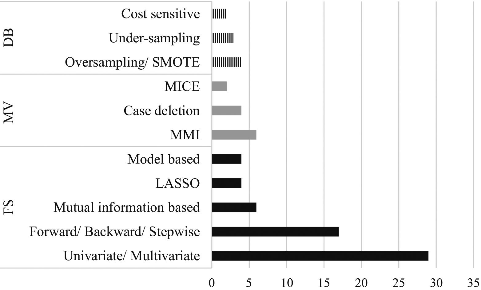

In the next section, the impact of each preprocessing approach is reported and discussed. Firstly, readmission discrimination performance is reported. Secondly, the time it takes to tune the Bayesian hyperparameters to optimise the ML models is discussed. The results reported are based on testing performance. Most of the machine learning algorithms assumed numerical inputs; hence the categorical variables were transformed into one-hot encoding before feature selection was made, after imputing the missing values. This technique is a common practice in many applications that deal with categorical data. This paper excluded deep learning analysis because preprocessing is implicitly integrated into the learning pipeline [66]. This study aimed to analyse the different preprocessing methods and the impact of each method on the prediction accuracy of the machine learning models.

4.3.1 Impact of missing value imputation

The two most common imputations used in readmission studies are MMI and MICE. Of the two, MMI is more preferred because it is easy to use and is not computationally heavy. Table 1 presents the impact of different missing value imputation methods on model performance.

Table 1
The impact of different missing value imputations on model performance

ML models	Criterion	Missing imputation algorithm
		Not applied	MMI	MICE
$k$ -NN	AUC	0.666	0.656	0.657
	Recall	0.552	0.533	0.529
	Precision	0.364	0.272	0.268
	Accuracy	0.750	0.658	0.656
LR	AUC	0.668	0.698	0.734
	Recall	0.655	0.580	0.623
	Precision	0.237	0.316	0.326
	Accuracy	0.567	0.698	0.702
NB	AUC	0.643	0.538	0.640
	Recall	0.897	0.981	0.970
	Precision	0.182	0.180	0.182
	Accuracy	0.268	0.198	0.214
DT	AUC	0.512	0.682	0.688
	Recall	0.069	0.506	0.503
	Precision	0.250	0.334	0.348
	Accuracy	0.799	0.731	0.742
RF	AUC	0.628	0.719	0.736
	Recall	0.552	0.632	0.645
	Precision	0.229	0.310	0.319
	Accuracy	0.591	0.682	0.690
SVM	AUC	0.626	0.703	0.722
	Recall	0.621	0.586	0.608
	Precision	0.214	0.306	0.310
	Accuracy	0.530	0.688	0.687
GBC	AUC	0.494	0.711	0.717
	Recall	0.759	0.595	0.607
	Precision	0.175	0.314	0.307
	Accuracy	0.323	0.694	0.684

According to the overall performance results listed in Table 1, studies that used missing value imputation had better overall performances in comparison with studies that did not (i.e., those that used CC analysis). For example, the imputation technique improved the AUC for LR, DT, RF, SVM, and GBC. The CC analysis or the removal of all the missing values led to poor prediction because the information removed might have contained some important information for prediction, and so some generalisation of the data could have been lost.

However, some of the classifiers such as $k$ -NN and NB were not affected by the CC analysis, as the AUC scores were almost similar to that of other imputation approaches, per Table 1. The $k$ -NN was not affected by any imputation approach, probably because it finds the most appropriate nearest neighbour throughout the entire dataset, regardless of data size. Meanwhile, the NB model uses the probabilistic approach and tries to minimise the outlier effect in the data. It works well with small data and hence, works well with CC analysis, as this approach reduces the amount of data.

In comparing MMI to MICE, interestingly, MICE techniques led to high AUC scores in almost all the machine learning models considered. The result could be due to the way MICE works, i.e., it allows some information from other variables by building a regression equation for the imputation process. This consideration of other predictors during the imputing process helps the researcher to select the most promising imputed values that in return help the overall prediction. Besides, LR is among the most affected models when used with MICE, where the difference in the AUC score in comparison to MMI was high (0.036). Since the foundation of the LR classifier is almost similar to MICE, these approaches share almost similar information (weight) with other variables. Therefore, it can be concluded that MICE is very suitable to use with LR.

On the other hand, MMI obtained a moderate AUC score. In most of the cases, it performed less than MICE but at the same time better than CC. This situation is because MMI simply imputes the mean or the mode of the overall data in a column, which often leads to bias, especially when there is a high range of values in specific features.

4.3.2 Impact of feature selection

The impact of different feature selection methods on the performance of the ML models was quantified, as shown in Table 2. This study considered the most frequently used feature selection category based on the studies. The results showed that the univariate Chi-Square filter method, the RFE wrapper method, and the LASSO embedded method were the most used feature selection categories. Therefore, these categories were compared.

Table 2
The impact of different feature selection algorithms on the ML model performance

ML models	Criterion	Feature scaling approach
		Not applied	LASSO	RFE	Univ. Chi-Square
$k$ -NN	AUC	0.657	0.664	0.690	0.681
	Recall	0.529	0.476	0.605	0.531
	Precision	0.268	0.288	0.289	0.296
	Accuracy	0.656	0.695	0.663	0.690
LR	AUC	0.734	0.735	0.698	0.732
	Recall	0.623	0.619	0.585	0.617
	Precision	0.326	0.325	0.314	0.325
	Accuracy	0.702	0.702	0.697	0.702
NB	AUC	0.640	0.669	0.661	0.669
	Recall	0.970	0.176	0.969	0.378
	Precision	0.182	0.448	0.183	0.342
	Accuracy	0.214	0.814	0.218	0.759
DT	AUC	0.688	0.685	0.660	0.683
	Recall	0.503	0.493	0.539	0.496
	Precision	0.348	0.349	0.318	0.334
	Accuracy	0.742	0.744	0.711	0.733
RF	AUC	0.736	0.736	0.697	0.734
	Recall	0.645	0.642	0.609	0.643
	Precision	0.319	0.320	0.305	0.317
	Accuracy	0.690	0.692	0.681	0.688
SVM	AUC	0.722	0.726	0.691	0.725
	Recall	0.608	0.626	0.655	0.623
	Precision	0.310	0.313	0.287	0.317
	Accuracy	0.687	0.687	0.634	0.692
GBC	AUC	0.717	0.729	0.697	0.733
	Recall	0.607	0.651	0.612	0.634
	Precision	0.307	0.309	0.298	0.320
	Accuracy	0.684	0.676	0.673	0.694

AUC was used to evaluate the overall performance of the models because it is the most commonly used measure in many readmission studies and imbalanced cases. The next performance measure used to examine the overall prediction performance was accuracy. Table 2 shows that studies that used feature selection selected better variables for the final prediction models and helped with the overall performance in comparison with studies that did not. For example, feature selection helped improve the performance of $k$ -NN, LR, NB, SVM and GBC (in terms of AUC) and increased the accuracy as compared to when no feature selection was used.

On the other hand, the performance of the AUC score for tree-based models such as DT and RF does not provide a significant difference either applying the feature selection or not. The reason for this case is that RF can work well with a large number of features as it builds the ensemble model from the subspace of data using DT. Hence, the tree-based models do not give much impact on any feature selection used.

Of all the feature selection methods, LASSO had the best performance (in terms of AUC and accuracy). LASSO outperformed other feature selection methods that used LR, NB, RF, and SVM. LASSO is an embedded technique, so it adds a constraint to the model to prevent overfitting and to improve generalisation. The weak features are forced to have a zero coefficient, so only the most impactful features are left. Also, this technique effectively captures dependencies between variables.

Conversely, RFE is underperformed compared to the other feature selection methods in most of the models. The reason for this case might be related to how RFE works. RFE recursively removes the features using a Greedy search to obtain the best subset. The remaining variables are then re-ranked by training a classifier. The weak features will be removed, so this could lead to reduced performance, as the weak features might still be useful when combined with other features. However, a past study justified that RFE is more suitable for small sample problems [23] and is less scalable to large datasets [48].

4.3.3 Impact of data balancing

This study considered resampling as the data balancing method, as it was the most used method in previous hospital readmission studies. Hence, this study compared the random under-sampling approach and the over-sampling approach. SMOTE was selected for the over-sampling approach because past readmission studies used this method the most. Most of these studies did not consider using data balancing. Hence, the performance of different data balancing methods was compared to highlight the importance of this method. Table 3 presents the result of this comparison.

Table 3
The impact of different data balancing approaches on model performance

ML models	Criterion	Data balancing approach
		Not applied	Under-sampling	Over-sampling
$k$ -NN	AUC	0.675	0.657	0.627
	Recall	0.018	0.529	0.102
	Precision	0.884	0.268	0.394
	Accuracy	0.821	0.656	0.808
LR	AUC	0.738	0.734	0.669
	Recall	0.130	0.623	0.222
	Precision	0.615	0.326	0.413
	Accuracy	0.827	0.702	0.801
NB	AUC	0.502	0.640	0.517
	Recall	0.996	0.970	0.902
	Precision	0.182	0.182	0.188
	Accuracy	0.187	0.214	0.272
DT	AUC	0.687	0.688	0.642
	Recall	0.060	0.503	0.287
	Precision	0.722	0.348	0.352
	Accuracy	0.825	0.742	0.774
RF	AUC	0.748	0.736	0.704
	Recall	0.095	0.645	0.219
	Precision	0.718	0.319	0.447
	Accuracy	0.829	0.690	0.809
SVM	AUC	0.683	0.722	0.680
	Recall	0.083	0.608	0.157
	Precision	0.706	0.310	0.484
	Accuracy	0.827	0.687	0.816
GBC	AUC	0.494	0.717	0.644
	Recall	0.759	0.607	0.292
	Precision	0.175	0.307	0.337
	Accuracy	0.323	0.684	0.767

It is justified that recall is as important as AUC score when evaluating the performance of the data balancing approach in handling the imbalanced data in a readmission dataset. Recall or TPR evaluates the extent to which the True Positive class has been correctly predicted out of the Total Positive classes. According to the overall performance results in Table 3, data balancing led to a more stable performance. Here, it can be seen that the AUC of some classifiers such as $k$ -NN, LR, RF, and GBC were higher when data balancing was not considered. However, most of the Recall values when not applying data balancing were quite low, indicating that the models failed to highlight the positive class. Also, the high accuracy in this situation shows that the model’s ability to predict the right targets came mostly from the negative class.

Of the data balancing approaches used, under-sampling had the best AUC score for all the classifiers. It can also be seen that under-sampling led to a more stable performance (in terms of recall and accuracy) in most of the cases. Based on Table 3, the Recall score was very low for almost all of the classifiers when SMOTE was used. This result is because under-sampling eliminates the sample of the majority class while oversampling replicates the majority class. The reason why under-sampling works well for this dataset is that the ratio of imbalanced data was nearly one-fifth of the overall dataset and comprised a handful of positive cases of around more than ten thousand instances. Additionally, the resampled negative class can represent the whole negative pattern of the data, so a stable performance is achieved.

4.3.4 Impact of feature scaling

Most of the studies did not report using feature scaling to predict readmission. Hence, this study investigated the impact of feature scaling on different classifiers. Table 4 presents the results of comparing the model performance when different data scaling approaches were used.

Table 4
The impact of different feature scaling approaches on model performance

ML models	Criterion	Feature scaling approach
		Not applied	Standardization	Normalization
$k$ -NN	AUC	0.653	0.657	0.617
	Recall	0.647	0.529	0.554
	Precision	0.249	0.268	0.238
	Accuracy	0.587	0.656	0.603
LR	AUC	0.735	0.734	0.733
	Recall	0.625	0.623	0.624
	Precision	0.326	0.326	0.324
	Accuracy	0.702	0.702	0.700
NB	AUC	0.646	0.640	0.645
	Recall	0.883	0.970	0.956
	Precision	0.193	0.182	0.184
	Accuracy	0.318	0.214	0.233
DT	AUC	0.675	0.688	0.686
	Recall	0.505	0.503	0.468
	Precision	0.317	0.348	0.356
	Accuracy	0.716	0.742	0.753
RF	AUC	0.736	0.736	0.735
	Recall	0.645	0.645	0.642
	Precision	0.321	0.319	0.320
	Accuracy	0.692	0.690	0.691
SVM	AUC	0.685	0.722	0.721
	Recall	0.622	0.608	0.630
	Precision	0.282	0.310	0.307
	Accuracy	0.649	0.687	0.680
GBC	AUC	0.721	0.717	0.729
	Recall	0.642	0.607	0.661
	Precision	0.305	0.307	0.312
	Accuracy	0.675	0.684	0.678

According to the results listed in Table 4, the feature scaling approaches did not show significant differences, despite specific models showing some minor differences. The reason might be due to the nature of the data itself. Feature scaling is very useful when the data has different scales across different features. This method turns all the features into comparable units. The studies reviewed only had ten numerical features, while the rest consisted of categorical features that had been transformed into a one-hot-encode label. Additionally, not all the numerical features had very large scales. For example, the range varied from [1–132], [0–6], [1–81], and [0–60] for the number of lab procedures, the number of procedures, the number of medications, and the number of diagnoses, respectively. Therefore, the small difference in scales caused feature scaling to have no significant impact on model performance.

Subsequently, moving into the details of the results, some of the findings may reveal some useful information. The Tree-based classifier, as can be seen in the Random Forest, was not affected by feature scaling, similar to some cases that used the Decision Tree. This result is possibly due to the splitting criteria that order the values in each attribute and then calculate the Gini or entropy split. Additionally, Naïve Bayes and Logistic Regression also presented consistent AUC values in Table 4. This result might also be due to the nature of the classifiers. For example, the model’s priors are determined from the count in each class, not by the actual values in Eq. (1). Hence, Naïve Bayes was not affected by feature scaling. For Logistic Regression, the coefficients represent the strength of the impact of each variable on the target variable. If the features do not affect the outcome, a broad range of data will render the corresponding coefficients of the regression algorithm small, so it will not affect the prediction as much.

Nevertheless, $k$ -NN was very much affected by feature scaling. This method uses Euclidean distance, which measures the nearest neighbours. This variable is affected by different scale magnitudes, and hence, the scaling procedure allows the attributes to have comparable units. Another classifier that is also affected by feature scaling, based on Table 4, is SVM. This classifier provides a decision boundary by measuring distance where it tries to maximise the margin between classes. In other words, attributes with very large numbers will dominate other attributes. According to the overall performance of each model, it can be concluded that data scaling led to improved classifier performance, especially the distance-based algorithms.

4.4 Bayesian hyperparameter optimisation tuning time

Under Bayesian optimisation, 100 maximum evaluations were set for each preprocessing combination and machine learning classifier to tune the hyperparameters. This setting was chosen based on several previous papers related to practical Bayesian optimisation [85, 75]. Then, studies that did not use feature selection and studies that used LASSO were compared because the overall tuning time for LASSO and other feature selection methods was not much different. Besides, LASSO also had the best performance. Table 5 shows the hyperparameter tuning time using Bayesian optimisation for different feature selection methods and data balancing techniques. The reported tuning times are presented in the format of hh: mm: ss indicating hours, minutes, and seconds, respectively.

Table 5
Bayesian hyperparameter tuning time (hours: minutes: seconds) for different feature selection methods and data balancing approaches

ML models	Feature selection	Data balancing
		Not apply	Under-sampling	Over-sampling
$k$ -NN	No FS	06 : 14 : 44	03 : 33 : 21	18 : 45 : 37
	LASSO	03 : 53 : 52	02 : 33 : 29	12 : 25 : 48
LR	No FS	01 : 38 : 42	00 : 56 : 51	05 : 47 : 24
	LASSO	00 : 08 : 57	00 : 12 : 09	00 : 06 : 16
DT	No FS	00 : 01 : 21	00 : 01 : 21	00 : 01 : 56
	LASSO	00 : 00 : 42	00 : 00 : 35	00 : 01 : 14
RF	No FS	02 : 58 : 22	01 : 16 : 53	03 : 59 : 49
	LASSO	01 : 27 : 50	00 : 53 : 31	02 : 38 : 28
GBC	No FS	11 : 03 : 28	03 : 30 : 15	20 : 25 : 18
	LASSO	06 : 40 : 46	02 : 13 : 30	22: 56 : 18

Naïve Bayes has no hyperparameters, so it does not need tuning. Therefore, this classifier was not included in the assessment. Table 5 shows a notably lower computational cost when LASSO feature selection is used. Additionally, data balancing using SMOTE oversampling had a very high computational cost, taking more than double the time it took for under-sampling approaches, especially for the $k$ -NN, RF, and GBC classifiers. The computational cost when no data balancing was used was in between undersampling and SMOTE techniques, with the under-sampling approach having a faster computational time. Table 6 shows the tuning time for the SVM hyperparameters. The time taken for the SVM hyperparameter optimisation was much longer than other machine learning models. Also, the exact time taken for SMOTE data balancing could not be determined because of its very long computation. Hence, for SVM, the same kernel was used for all cases, which is the RBF kernel. This kernel was chosen due to its performance and because it is the most commonly used kernel for SVM models in readmission studies [92, 50, 102].

Table 6

Bayesian hyperparameter tuning time (hours: minutes: seconds) for the SVM model

ML model	Feature selection	Data balancing
		Under-sampling	Over-sampling
SVM	No FS	56 : 01 : 34	–
	LASSO	28 : 10 : 13	${}^{*}$ 737 : 22 : 17

${}^{*}$ Computation time at the second evaluation.

Of the ML models, SVM demonstrated the highest computational cost, especially in combination with SMOTE and not apply feature selection. GBC and $k$ -NN dominated next after SVM, but in most of the cases, $k$ -NN took longer to optimise the hyperparameters. DT required little computational cost for optimising the hyperparameters, albeit when not apply feature selection and considering the over-sampling approach. Hence, DT is very suitable for fast decision making and predictions. In sum, the Bayesian optimisation of the hyperparameters with feature selection and under-sampling required much less time and lesser computational costs, regardless of the ML model used.

5. Discussions

Preprocessing is a challenging task, especially when the data is noisy, severely skewed, and contains hundreds of attributes. In this study, four preprocessing approaches were considered, which are missing value imputation, feature selection, data balancing, and feature scaling. The combination of all these methods was evaluated based on the AUC, precision, recall, and accuracy of all the ML classifiers.

Missing value imputation is an important task, especially when there is a huge number of missing instances. In most of the readmission studies, MMI was used because it is easy to use and has a low computational cost. However, this study showed that using multiple imputations (i.e. MICE) could improve the overall classification performance, as shown in Table 1. This is because MICE allows the use of some information (e.g., the degree of the relationship between other attributes) for the imputation process. These imputation values can then be used for imputing other attributes.

Secondly, feature selection was shown to improve the performance of the ML models. Even though in some cases, the performance of the models that did not use feature selection was almost the same as that of models using feature selection, feature selection still helped reduce the overall computational cost. Of the feature selection methods considered in this study, LASSO showed the most outstanding performance. The reason for this result is that LASSO removes weak features by shrinking them to zero coefficients, hence only leaving the most impactful features.

Thirdly, data balancing was proven crucial for handling imbalanced data. It can help identify the behaviour of minority samples (i.e. readmitted patients). Resampling techniques were studied, namely undersampling and oversampling, using SMOTE. Table 3 shows that data balancing helped produce a more stable performance compared to when no data balancing was used. Another important finding is that under-sampling outperformed SMOTE in most of the cases in this study. This is because of the nature of the data, which can be considered not too heavily skewed. Besides, at the same time, the resampling of negative instances could represent the whole negative pattern in the data.

Finally, the last preprocessing approach considered in this study was feature scaling. This method is also an essential step to apply when the data is not in the same range. The commonly used feature scaling approaches are standardisation and normalisation. Based on the findings in Table 4, it can be concluded that feature scaling had no significant impact on classifier performance. This is mainly because of the nature of the data used in this study, which has a numerical data range that is not too large. However, the ML models in this study that used the NB, LR, DT, RF, and GBC classifiers were unaffected by scaling methods while those that used the $k$ -NN and SVM classifiers were very much affected. This result is mainly due to how these classifiers work, as explained in Section 4.3.4 above.

On the other hand, hyperparameter optimisation is also an important process in predictive modelling. This study used Bayesian hyperparameter optimisation, which is an effective way to tune hyperparameters. Hence, the effect of the computational time of different preprocessing approaches on the performance of different ML models was investigated to provide the researcher with some insight on the suitability of this optimisation method with different pipelines.

Based on the experiment involving each approach, the hyperparameter tuning for every ML model together with SMOTE data balancing led to triple the computational costs compared to the under-sampling approach. In the same way, every ML model that used hyperparameter tuning with no feature selection also had higher computational costs than the models that did not use feature selection. The computational cost increased when both the above approaches were combined (i.e. no feature selection and SMOTE). On the other hand, the hyperparameter tuning also differs for each ML model. Regardless of the preprocessing approach selected, SVM took a very long time to tune the hyperparameters. In contrast, DT took a very short time to tune the hyperparameters. Hence, DT is very suitable for fast decision making and fast predictions.

Overall, the results showed a modest to good testing. The results might be incomparable across other related studies, as they varied depending on the target population or disease, the availability of the features in a database, and the length of readmissions. When classification performance and computational cost were combined, RF with MICE imputation, LASSO feature selection and under-sampling framework gave the best performance. Additionally, the second proposed combination were the ML classifiers of LR, GBC and SVM with MICE imputation, LASSO embedded feature selection and under-sampling framework. The third best combination that has a similar pipeline for ML classifiers above are MICE imputation, Univariate Chi-Square filter feature selection and under-sampling framework.

6. Conclusion and further study

This study evaluated the effect of preprocessing and machine learning pipelines on hospital readmission prediction. It can be concluded that the most promising pipeline was the combination of the RF classifier for the ML model with MICE imputation, LASSO feature selection, and under-sampling data balancing as the preprocessing framework. The same preprocessing method also works well for other ML classifiers such as GBC, SVM, and LR. Machine learning has emerged as a promising approach in recent years, more so than other statistical modelling techniques, especially for predicting readmission risk. Hence, most of the existing studies had prepared an overall workflow limited to the baseline of the models. Also, these studies tended to follow established procedures.

Based on the ML prediction studies reviewed, most did not focus on preprocessing approaches. Overall, most of the studies used feature selection with only 20% applying missing value imputation and 13% addressing the imbalanced class problem. However, missing value imputation could be irrelevant in some cases due to the completeness of the data in hand. In contrast, class imbalance is a well-known problem that affects overall discrimination performance. Most of the studies used MMI as the missing value imputation approach, which is also the simplest. Meanwhile, the univariate feature selection was the most commonly used approach.

Bayesian optimisation has increasingly been used in many applications in recent years, as it helps choose the appropriate set of hyperparameters for each model. The right combination of preprocessing methods may help reduce computational costs and improve discrimination performance. This study only considered a maximum evaluation of 100 due to the computational cost. For future research, the number of assessments might be increased to further improve the selection of hyperparameters. Moreover, a comparative study could be done to assess the impact of different numbers of evaluations on different datasets. In sum, this study considered the effect of selected preprocessing methods on the performance of the machine learning classifiers. Besides, this study only considered existing datasets, so the results might not generalise the overall performance of readmission prediction. Hence, further comparative studies should be done to assess the impact of other available preprocessing techniques with different readmission datasets to better generalise the effect of preprocessing pipelines on predictive performance.

Another challenge in readmission prediction refers to the curse of dimensionality due to the large data sets involved with many potential predictor variables. Theoretically, the incorporation of additional variables into the model yielded better prediction, thus enabling information storage. Nonetheless, it rarely helps in practical as the convergence to obtain those solutions might be increasingly slow due to the potential presence of noise and redundant variables [71]. Solutions that had effectively managed the curse of dimensionality were feature selection and dimensionality reduction, wherein both had minimised the input variable. The capability of input variables reduction displayed in this study using feature selection techniques is applicable for supervised learning [67]. Feature selection had enhanced the overall prediction performance in this study. On the other hand, the dimensionality reduction methods, such as principal component analysis (PCA), is applicable for both supervised and unsupervised data and may be further investigated by future researchers in comparative studies to address the curse of dimensionality, and to determine the suitability of these approaches in studies related to hospital readmission.

The prediction of hospital readmission is a naturally complex problem, as explained in [52]. Besides, predicting hospital admission is not as easy as predicting death, so high discrimination performance is also not easily achieved [9]. The machine learning models might have limited overall performance because of the lack of relevant data, although more complex models have been used. With the improvements to the whole machine learning framework, which includes the preprocessing pipeline, prediction performance can also be improved. Meanwhile, although it is known that no one model fits all, this study offered some insight into the importance of applying preprocessing for machine learning models. Hence, future studies could refer to this study to explore other preprocessing pipelines for machine learning classifiers, especially for readmission tasks, and for other medical problems in general.

Footnotes

Acknowledgments

The financial support received from the University of Malaya (IIRG004B-19HWB), Universiti Kebangsaan Malaysia, and the Ministry of Higher Education Malaysia are gratefully acknowledged.

Conflict of interest

The authors declare no conflict of interest.

References

AbdelRahman

S.E.

Zhang

Bray

B.E.

and Kawamoto

, A three-step approach for the derivation and validation of high-performing predictive models using an operational dataset: congestive heart failure readmission case study, BMC Medical Informatics and Decision Making 14(1) (2014), 41.

Agrawal

Chen

C.-B.

Dravenstott

R.W.

Strömblad

C.T.

Schmid

J.A.

Darer

J.D.

Devapriya

and Kumara

, Predicting patients at risk for 3-day postdischarge readmissions, ed visits, and deaths, Medical Care 54(11) (2016), 1017–1023.

Ali

Shamsuddin

S.M.

Ralescu

A.L.

et al., Classification with class imbalance problem: a review, Int. J. Advance Soft Compu. Appl 7(3) (2015), 176–204.

Ali

A.M.

and Gibbons

C.E.

, Predictors of 30-day hospital readmission after hip fracture: a systematic review, Injury 48(2) (2017), 243–252.

Allen

L.A.

Tomic

K.E.S.

Smith

D.M.

Wilson

K.L.

and Agodoa

, Rates and predictors of 30-day readmission among commercially insured and medicaid-enrolled patients hospitalized with systolic heart failure, Circulation: Heart Failure 5(6) (2012), 672–679.

Allison

G.M.

Muldoon

E.G.

Kent

D.M.

Paulus

J.K.

Ruthazer

Ren

and Snydman

D.R.

, Prediction model for 30-day hospital readmissions among patients discharged receiving outpatient parenteral antibiotic therapy, Clinical Infectious Diseases 58(6) (2013), 812–819.

Amalakuhan

Kiljanek

Parvathaneni

Hester

Cheriyath

and Fischman

, A prediction model for copd readmissions: catching up, catching our breath, and improving a national problem, Journal of Community Hospital Internal Medicine Perspectives 2(1) (2012), 9915.

Ambler

Omar

R.Z.

and Royston

, A comparison of imputation techniques for handling missing predictor values in a risk model with a binary outcome, Statistical Methods in Medical Research 16(3) (2007), 277–298.

Artetxe

Beristain

and Grana

, Predictive models for hospital readmission risk: a systematic review of methods, Computer Methods and Programs in Biomedicine 164 (2018), 49–64.

10.

A.G.

McAlister

F.A.

Bakal

J.A.

Ezekowitz

Kaul

and van Walraven

, Predicting the risk of unplanned readmission or death within 30 days of discharge after a heart failure hospitalization, American Heart Journal 164(3) (2012), 365–372.

11.

Azur

M.J.

Stuart

E.A.

Frangakis

and Leaf

P.J.

, Multiple imputation by chained equations: what is it and how does it work? International Journal of Methods in Psychiatric Research 20(1) (2011), 40–49.

12.

Baltodano

P.A.

Webb-Vargas

Soares

Hicks

Cooney

C.M.

Cornell

Burce

Pawlik

and Eckhauser

, A validated, risk assessment tool for predicting readmission after open ventral hernia repair, Hernia 20(1) (2016), 119–129.

13.

Bergstra

Yamins

and Cox

D.D.

, Hyperopt: A python library for optimizing the hyperparameters of machine learning algorithms, in: Proceedings of the 12th Python in Science Conference, Citeseer, 2013, pp. 13–20.

14.

Bergstra

J.S.

Bardenet

Bengio

and Kégl

, Algorithms for hyper-parameter optimization, in: Advances in Neural Information Processing Systems, 2011, pp. 2546–2554.

15.

Berman

Tandra

Forssell

Vuppalanchi

Burton

J.R.

Jr Nguyen

Mullis

Kwo

and Chalasani

, Incidence and predictors of 30-day readmission among patients hospitalized for advanced liver disease, Clinical Gastroenterology and Hepatology 9(3) (2011), 254–259.

16.

Bradford

Shah

B.M.

Shane

Wachi

and Sahota

, Patient and clinical characteristics that heighten risk for heart failure readmission, Research in Social and Administrative Pharmacy 13(6) (2017), 1070–1081.

17.

Brauer

D.G.

Lyons

S.A.

Keller

M.R.

Mutch

M.G.

Colditz

G.A.

and Glasgow

S.C.

, Simplified risk prediction indices do not accurately predict 30-day death or readmission after discharge following colorectal surgery, Surgery 165(5) (2019), 882–888.

18.

Breiman

, Random forests, Machine Learning 45(1) (2001), 5–32.

19.

Casalini

Salvetti

Memmini

Lucaccini

Massimetti

Lopalco

P.L.

and Privitera

G.P.

, Unplanned readmissions within 30 days after discharge: improving quality through easy prediction, International Journal for Quality in Health Care 29(2) (2017), 256–261.

20.

Chawla

N.V.

Bowyer

K.W.

Hall

L.O.

and Kegelmeyer

W.P.

, Smote: synthetic minority over-sampling technique, Journal of Artificial Intelligence Research 16 (2002), 321–357.

21.

Che

Purushotham

Khemani

and Liu

, Interpretable deep models for icu outcome prediction, in: AMIA Annual Symposium Proceedings, Vol. 2016, American Medical Informatics Association, 2016, p. 371.

22.

Chen

S.Y.

Stem

Cerullo

Canner

J.K.

Gearhart

S.L.

Safar

Fang

S.H.

and Efron

J.E.

, Predicting the risk of readmission from dehydration after ileostomy formation: the dehydration readmission after ileostomy prediction score, Diseases of the Colon & Rectum 61(12) (2018), 1410–1417.

23.

Chen

X.-w.

and Jeong

J.C.

, Enhanced recursive feature elimination, in: Sixth International Conference on Machine Learning and Applications (ICMLA 2007), IEEE, 2007, pp. 429–435.

24.

Claesen

and De Moor

, Hyperparameter search in machine learning, arXiv preprint arXiv:1502.02127, 2015.

25.

Collins

Abbass

I.M.

Harvey

Suehs

Uribe

Bouchard

Prewitt

DeLuzio

and Allen

, Predictors of all-cause 30 day readmission among medicare patients with type 2 diabetes, Current Medical Research and Opinion 33(8) (2017), 1517–1523.

26.

Conroy

Eshelman

Potes

and Xu-Wilson

, A dynamic ensemble approach to robust classification in the presence of missing data, Machine Learning 102(3) (2016), 443–463.

27.

Cui

Metge

Moffatt

Oppenheimer

and Forget

E.L.

, Development and validation of a predictive model for all-cause hospital readmissions in winnipeg, canada, Journal of Health Services Research & Policy 20(2) (2015), 83–91.

28.

Dharmarajan

Hsieh

A.F.-C.

Lin

Bueno

H.C.B.

Ross

J.S.

Horwitz

L.I.

Barreto-Filho

J.A.S.

Kim

N.I.

Bernheim

S.M.

Suter

L.G.

Drye

E.E.

and Krumholz

H.M.

, Diagnoses and timing of 30-day readmissions after hospitalization for heart failure, acute myocardial infarction, or pneumonia, JAMA 309(4) (2013), 355–363.

29.

Donders

A.R.T.

Van Der Heijden

G.J.

Stijnen

and Moons

K.G.

, A gentle introduction to imputation of missing values, Journal of Clinical Epidemiology 59(10) (2006), 1087–1091.

30.

Dorajoo

S.R.

See

Chan

C.T.

Tan

J.Z.

Tan

D.S.Y.

Abdul Razak

S.M.B.

Ong

T.T.

Koomanan

Yap

C.W.

and Chan

, Identifying potentially avoidable readmissions: a medication-based 15-day readmission risk stratification algorithm, Pharmacotherapy: The Journal of Human Pharmacology and Drug Therapy 37(3) (2017), 268–277.

31.

Elhassan

and Aljurf

, Classification of imbalance data using tomek link (t-link) combined with random under-sampling (rus) as a data reduction method, Global Journal of Technology & Optimization, 2017.

32.

Felix

E.A.

and Lee

S.P.

, Systematic literature review of preprocessing techniques for imbalanced data, IET Software 13(6) (2019), 479–496.

33.

Fernandez-Gasso

Hernando-Arizaleta

Palomar-Rodríguez

J.A.

Abellán-Pérez

M.V.

and Pascual-Figal

D.A.

, Trends, causes and timing of 30-day readmissions after hospitalization for heart failure: 11-year population-based analysis with linked data, International Journal of Cardiology 248 (2017), 246–251.

34.

Fisher

S.R.

Graham

J.E.

Krishnan

and Ottenbacher

K.J.

, Predictors of 30-day readmission following inpatient rehabilitation for patients at high risk for hospital readmission, Physical Therapy 96(1) (2016), 62–70.

35.

Frizzell

J.D.

Liang

Schulte

P.J.

Yancy

C.W.

Heidenreich

P.A.

Hernandez

A.F.

Bhatt

D.L.

Fonarow

G.C.

and Laskey

W.K.

, Prediction of 30-day all-cause readmissions in patients hospitalized for heart failure: comparison of machine learning and other statistical approaches, JAMA Cardiology 2(2) (2017), 204–209.

36.

Futoma

Morris

and Lucas

, A comparison of models for predicting early hospital readmissions, Journal of Biomedical Informatics 56 (2015), 229–238.

37.

García-Pérez

Linertová

Lorenzo-Riera

Vázquez-Díaz

Duque-González

and Sarría-Santamera

, Risk factors for hospital readmissions in elderly patients: a systematic review, QJM: An International Journal of Medicine 104(8) (2011), 639–651.

38.

Garciarena

and Santana

, An extensive analysis of the interaction between missing data types, imputation methods, and supervised classifiers, Expert Systems with Applications 89 (2017), 52–65.

39.

Garrison

G.M.

Mansukhani

M.P.

and Bohn

, Predictors of thirty-day readmission among hospitalized family medicine patients, J Am Board Fam Med 26(1) (2013), 71–77.

40.

Géron

, Hands-on machine learning with scikit-learn and tensorflow: concepts, tools, and techniques to build intelligent systems o’reilly media, Sebastopol, CA, 2017, pp. 54–56.

41.

Golas

S.B.

Shibahara

Agboola

Otaki

Sato

Nakae

Hisamitsu

Kojima

Felsted

Kakarmath

et al., A machine learning model to predict the risk of 30-day readmissions in patients with heart failure: a retrospective analysis of electronic medical records data, BMC Medical Informatics and Decision Making 18(1) (2018), 44.

42.

Golmohammadi

and Radnia

, Prediction modeling and pattern recognition for patient readmission, International Journal of Production Economics 171 (10 2015), 151–161.

43.

Greenwald

J.L.

Cronin

P.R.

Carballo

Danaei

and Choy

, A novel model for predicting rehospitalization risk incorporating physical function, cognitive status, and psychosocial support using natural language processing, Medical Care 55(3) (2017), 261–266.

44.

Hammoudeh

Al-Naymat

Ghannam

and Obied

, Predicting hospital readmission among diabetics using deep learning, Procedia Computer Science 141 (2018), 484–489.

45.

Hasan

Meltzer

D.O.

Shaykevich

S.A.

Bell

C.M.

Kaboli

P.J.

Auerbach

A.D.

Wetterneck

T.B.

Arora

V.M.

Zhang

and Schnipper

J.L.

, Hospital readmission in general medicine patients: a prediction model, Journal of General Internal Medicine 25(3) (2010), 211–219.

46.

Hatipoğlu

Wells

B.J.

Chagin

Joshi

Milinovich

and Rothberg

M.B.

, Predicting 30-day all-cause readmission risk for subjects admitted with pneumonia at the point of care, Respiratory Care 63(1) (2018), 43–49.

47.

Hosseinzadeh

Izadi

Verma

Precup

and Buckeridge

, Assessing the predictability of hospital readmission using machine learning, in: Twenty-Fifth IAAI Conference, 2013.

48.

Jain

and Singh

, Feature selection and classification systems for chronic disease prediction: a review, Egyptian Informatics Journal 19(3) (2018), 179–189.

49.

Jamei

Nisnevich

Wetchler

Sudat

and Liu

, Predicting all-cause risk of 30-day hospital readmission using artificial neural networks, PloS One 12(7) (2017), e0181173.

50.

Jiang

Chin

K.-S.

and Tsui

K.L.

, An integrated machine learning framework for hospital readmission prediction, Knowledge-Based Systems 146 (2018), 73–90.

51.

Jovanovic

Radovanovic

Vukicevic

Van Poucke

and Delibasic

, Building interpretable predictive models for pediatric hospital readmission using tree-lasso logistic regression, Artificial Intelligence in Medicine 72 (2016), 12–21.

52.

Kansagara

Englander

Salanitro

Kagen

Theobald

Freeman

and Kripalani

, Risk prediction models for hospital readmission: a systematic review, Jama 306(15) (2011), 1688–1698.

53.

Kaur

Naessens

J.M.

Hanson

A.C.

Fryer

Nemergut

M.E.

and Tripathi

, Proper: development of an early pediatric intensive care unit readmission risk prediction tool, Journal of Intensive Care Medicine 33(1) (2018), 29–36.

54.

Laudicella

Donni

P.L.

and Smith

P.C.

, Hospital readmission rates: signal of failure or success? Journal of Health Economics 32(5) (2013), 909–921.

55.

Leary

J.C.

Price

L.L.

Scott

C.E.

Kent

Wong

J.B.

and Freund

K.M.

, Developing prediction models for 30-day unplanned readmission among children with medical complexity, Hospital Pediatrics 9(3) (2019), 201–208.

56.

Lee

E.W.

, Selecting the best prediction model for readmission, Journal of Preventive Medicine and Public Health 45(4) (2012), 259.

57.

D.-C.

Liu

C.-W.

and Hu

S.C.

, A learning method for the class imbalance problem with medical data sets, Computers in Biology and Medicine 40(5) (2010), 509–518.

58.

Lim

N.-K.

Lee

S.E.

Lee

H.-Y.

Cho

H.-J.

Choe

W.-S.

Kim

Choi

J.O.

Jeon

E.-S.

Kim

M.-S.

Kim

J.-J.

et al., Risk prediction for 30-day heart failure-specific readmission or death after discharge: data from the korean acute heart failure (korahf) registry, Journal of Cardiology 73(2) (2019), 108–113.

59.

Lin

K.-P.

Chen

P.-C.

Huang

L.-Y.

Mao

H.-C.

and Chan

D.-C.D.

, Predicting inpatient readmission and outpatient admission in elderly: a population-based cohort study, Medicine 95(16) (2016).

60.

Lokanayaki

and Malathi

, Data preprocessing for liver dataset using smote, International Journal of Advanced Research in Computer Science and Software Engineering 3(11) (2013).

61.

López-Aguilà

Contel

Farre

Campuzano

and Rajmil

, Predictive model for emergency hospital admission and 6-month readmission, The American Journal of Managed Care 17(9) (2011), 348–357.

62.

Low

L.L.

Liu

Wang

Thumboo

Ong

M.E.H.

and Lee

K.H.

, Predicting 30-day readmissions in an asian population: building a predictive model by incorporating markers of hospitalization severity, PLoS One 11(12) (2016), e0167413.

63.

and Chu

, Adaptive ensemble undersampling-boost: a novel learning framework for imbalanced data, Journal of Systems and Software 132 (2017), 272–282.

64.

Mani

and Zhang

, knn approach to unbalanced data distributions: a case study involving information extraction, in: Proceedings of Workshop on Learning from Imbalanced Datasets, Vol. 126, 2003.

65.

McLaren

D.P.

Jones

Plotnik

Zareba

McIntosh

Alexis

Chen

Block

Lowenstein

C.J.

and Kutyifa

, Prior hospital admission predicts thirty-day hospital readmission for heart failure patients, Cardiology Journal 23(2) (2016), 155–162.

66.

Min

and Wang

, Predictive modeling of the hospital readmission risk from patients’ claims data using machine learning: a case study on copd, Scientific Reports 9(1) (2019), 2362.

67.

Miner

Elder IV

Fast

Hill

Nisbet

and Delen

, Practical text mining and statistical analysis for non-structured text data applications, Academic Press, 2012.

68.

Morris

J.N.

Howard

E.P.

Steel

Schreiber

Fries

B.E.

Lipsitz

L.A.

and Goldman

, Predicting risk of hospital and emergency department use for home care elderly persons through a secondary analysis of cross-national data, BMC Health Services Research 14(1) (2014), 519.

69.

Mortazavi

B.J.

Downing

N.S.

Bucholz

E.M.

Dharmarajan

Manhapra

S.-X.

Negahban

S.N.

and Krumholz

H.M.

, Analysis of machine learning techniques for heart failure readmissions, Circulation: Cardiovascular Quality and Outcomes 9(6) (2016), 629–640.

70.

Nijhawan

A.E.

Clark

Kaplan

Moore

Halm

E.A.

and Amarasingham

, An electronic medical record-based model to predict 30-day risk of readmission and death among hiv-infected inpatients, JAIDS Journal of Acquired Immune Deficiency Syndromes 61(3) (2012), 349–358.

71.

Nisbet

Elder

and Miner

, Handbook of statistical analysis and data mining applications, Academic Press, 2009.

72.

Ouanes

Schwebel

Français

Bruel

Philippart

Vesin

Soufir

Adrie

Garrouste-Orgeas

Timsit

J.-F.

et al., A model to predict short-term death or readmission after intensive care unit discharge, Journal of Critical Care 27(4) (2012), 422–e1.

73.

Padhukasahasram

Reddy

C.K.

and Lanfear

D.E.

, Joint impact of clinical and behavioral variables on the risk of unplanned readmission and death after a heart failure hospitalization, PloS One 10(6) (2015), e0129553.

74.

Pereira

Choquet

Perozziello

Wargon

Juillien

Colosi

Hellmann

Ranaivoson

and Casalino

, Unscheduled-return-visits after an emergency department (ed) attendance and clinical link between both visits in patients aged 75 years and over: a prospective observational study, PloS One 10(4) (2015), e0123803.

75.

Qin

Klabjan

and Russo

, Improving the expected improvement algorithm, in: Advances in Neural Information Processing Systems, 2017, pp. 5381–5391.

76.

Rao

Barrow

Vuik

Darzi

and Aylin

, Systematic review of hospital readmissions in stroke patients, Stroke research and treatment, 2016, pp. 1–11.

77.

Raschka

, Python machine learning, Packt Publishing Ltd, 2015.

78.

Remeseiro

and Bolon-Canedo

, A review of feature selection methods in medical applications, Computers in Biology and Medicine 112 (2019), 103375.

79.

Rojas

J.C.

Carey

K.A.

Edelson

D.P.

Venable

L.R.

Howell

M.D.

and Churpek

M.M.

, Predicting intensive care unit readmission with machine learning using electronic health record data, Annals of the American Thoracic Society 15(7) (2018), 846–853.

80.

Ross

J.S.

Mulvey

G.K.

Stauffer

Patlolla

Bernheim

S.M.

Keenan

P.S.

and Krumholz

H.M.

, Statistical models and patient predictors of readmission for heart failure: a systematic review, Archives of Internal Medicine 168(13) (2008), 1371–1386.

81.

Sfoungaristos

Hidas

Gofrit

O.N.

Rosenberg

Yutkin

Landau

E.H.

Pode

and Duvdevani

, A novel model to predict the risk of readmission in patients with renal colic, Journal of Endourology 28(8) (2014), 1011–1015.

82.

Shadmi

Flaks-Manov

Hoshen

Goldman

Bitterman

and Balicer

R.D.

, Predicting 30-day readmissions with preadmission electronic health record data, Medical Care 53(3) (2015), 283–289.

83.

Shahriari

Swersky

Wang

Adams

R.P.

and De Freitas

, Taking the human out of the loop: a review of bayesian optimization, Proceedings of the IEEE 104(1) (2015), 148–175.

84.

Smith

L.N.

Makam

A.N.

Darden

Mayo

Das

S.R.

Halm

E.A.

and Nguyen

O.K.

, Acute myocardial infarction readmission risk prediction models: a systematic review of model performance, Circulation: Cardiovascular Quality and Outcomes 11(1) (2018).

85.

Snoek

Larochelle

and Adams

R.P.

, Practical bayesian optimization of machine learning algorithms, in: Advances in Neural Information Processing Systems, 2012, pp. 2951–2959.

86.

Sterne

J.A.

White

I.R.

Carlin

J.B.

Spratt

Royston

Kenward

M.G.

Wood

A.M.

and Carpenter

J.R.

, Multiple imputation for missing data in epidemiological and clinical research: potential and pitfalls, Bmj 338 (2009), b2393.

87.

Strack

DeShazo

J.P.

Gennings

Olmo

J.L.

Ventura

Cios

K.J.

and Clore

J.N.

, Impact of hba1c measurement on hospital readmission rates: analysis of 70,000 clinical database patient records, BioMed research international, 2014, 2014.

88.

Tabak

Y.P.

Sun

Nunez

C.M.

Gupta

and Johannes

R.S.

, Predicting readmission at early hospitalization using electronic clinical data: an early readmission risk score, Medical Care 55(3) (2017), 267.

89.

Thomson

Fletcher

Valencia

and Sharma

, Readmission to the intensive care unit following cardiac surgery: a derived and validated risk prediction model in 4,869 patients, Journal of Cardiothoracic and Vascular Anesthesia 32(6) (2018), 2685–2691.

90.

Tong

Erdmann

Daldalian

and Esposito

, Comparison of predictive modeling approaches for 30-day all-cause non-elective readmission risk, BMC Medical Research Methodology 16(1) (2016), 26.

91.

Tulloch

David

and Thornicroft

, Exploring the predictors of early readmission to psychiatric hospital, Epidemiology and Psychiatric Sciences 25(2) (2016), 181–193.

92.

Turgeman

and May

J.H.

, A mixed-ensemble model for hospital readmission, Artificial Intelligence in Medicine 72 (2016), 72–82.

93.

van Diepen

Graham

M.M.

Nagendran

and Norris

C.M.

, Predicting cardiovascular intensive care unit readmission after cardiac surgery: derivation and validation of the alberta provincial project for outcomes assessment in coronary heart disease (approach) cardiovascular intensive care unit clinical prediction model from a registry cohort of 10,799 surgical cases, Critical Care 18(6) (2014), 651.

94.

van Walraven

Dhalla

I.A.

Bell

Etchells

Stiell

I.G.

Zarnke

Austin

P.C.

and Forster

A.J.

, Derivation and validation of an index to predict early death or unplanned readmission after discharge from hospital to the community, Cmaj 182(6) (2010), 551–557.

95.

Viegas

Salgado

C.M.

Curto

Carvalho

J.P.

Vieira

S.M.

and Finkelstein

S.N.

, Daily prediction of icu readmissions using feature engineering and ensemble fuzzy modeling, Expert Systems with Applications 79 (2017), 244–253.

96.

Vigod

S.N.

Kurdyak

P.A.

Seitz

Herrmann

Fung

Lin

Perlman

Taylor

V.H.

Rochon

P.A.

and Gruneir

, Readmit: a clinical risk index to predict 30-day readmission after discharge from acute psychiatric units, Journal of Psychiatric Research 61 (2015), 205–213.

97.

Wallmann

Llorca

Gómez-Acebo

Ortega

Á.C.

Roldan

F.R.

and Dierssen-Sotos

, Prediction of 30-day cardiac-related-emergency-readmissions using simple administrative hospital data, International Journal of Cardiology 164(2) (2013), 193–200.

98.

Walsh

and Hripcsak

, The effects of data sources, cohort selection, and outcome definition on a predictive model of risk of thirty-day hospital readmissions, Journal of Biomedical Informatics 52 (2014), 418–426.

99.

Wang

Cui

Chen

Avidan

Abdallah

A.B.

and Kronzer

, Cost-sensitive deep learning for early readmission prediction at a major hospital, Canada Proc. BIOKDD (17) (2017).

100.

Wang

Cui

Chen

Avidan

Abdallah

A.B.

and Kronzer

, Predicting hospital readmission via cost-sensitive deep learning, IEEE/ACM Transactions on Computational Biology and Bioinformatics (TCBB) 15(6) (2018), 1968–1978.

101.

Watson

A.J.

O’Rourke

Jethwani

Cami

Stern

T.A.

Kvedar

J.C.

Chueh

H.C.

and Zai

A.H.

, Linking electronic health record-extracted psychosocial data in real-time to risk of readmission for heart failure, Psychosomatics 52(4) (2011), 319–327.

102.

Wolff

Graña

Ríos

S.A.

and Yarza

M.B.

, Machine learning readmission risk modeling: A pediatric case study, BioMed research international, 2019, 2019.

103.

Yen

S.-J.

and Lee

Y.-S.

, Cluster-based under-sampling approaches for imbalanced data distributions, Expert Systems with Applications 36(3) (2009), 5718–5727.

104.

Zapatero

Barba

Marco

Hinojosa

Plaza

Losa

J.E.

and Canora

, Predictive model of readmission to internal medicine wards, European Journal of Internal Medicine 23(5) (2012), 451–456.

105.

Zhao

and Yoo

, A systematic review of highly generalizable risk factors for unplanned 30-day all-cause hospital readmissions, Journal of Health & Medical Informatics 8 (9 2017).

106.

Zheng

Zhang

Yoon

S.W.

Lam

S.S.

Khasawneh

and Poranki

, Predictive modeling of hospital readmissions using metaheuristics and data mining, Expert Systems with Applications 42(20) (2015), 7110–7120.

107.

Zolfaghar

Verbiest

Agarwal

Meadem

Chin

S.-C.

Roy

S.B.

Teredesai

Hazel

Amoroso

and Reed

, Predicting risk-of-readmission for congestive heart failure patients: A multi-layer approach, arXiv preprint arXiv:1306.2094, 2013.

Predictive modelling of hospital readmission: Evaluation of different preprocessing techniques on machine learning classifiers

Abstract

Keywords

1. Introduction

3.1 Preprocessing pipeline

3.1.1 Missing value imputation

3.1.2 Feature selection

3.1.3 Data balancing

3.1.4 Feature scaling

4.1 Dataset description

4.2 Experimental evaluation

4.3 Preprocessing performances

Table 1 The impact of different missing value imputations on model performance

Table 2 The impact of different feature selection algorithms on the ML model performance

Table 3 The impact of different data balancing approaches on model performance

Table 4 The impact of different feature scaling approaches on model performance

Table 5 Bayesian hyperparameter tuning time (hours: minutes: seconds) for different feature selection methods and data balancing approaches

6. Conclusion and further study

Footnotes

Acknowledgments

Conflict of interest

References

Table 1
The impact of different missing value imputations on model performance

Table 2
The impact of different feature selection algorithms on the ML model performance

Table 3
The impact of different data balancing approaches on model performance

Table 4
The impact of different feature scaling approaches on model performance

Table 5
Bayesian hyperparameter tuning time (hours: minutes: seconds) for different feature selection methods and data balancing approaches