Sparse non-negative matrix factorization for uncertain data clustering

Abstract

We consider the problem of clustering a set of uncertain data, where each data consists of a point-set indicating its possible locations. The objective is to identify the representative for each uncertain data and group them into $k$ clusters so as to minimize the total clustering cost. Different from other models, our model does not assume that there is a probability distribution for each uncertain data. Thus, all possible locations need to be considered to determine the representative. Existing methods for this problem are either impractical or have difficulty to handle large-scale datasets due to their pairwise-distance based global search strategy and expensive optimization computation. In this paper, we propose a novel sparse Non-negative Matrix Factorization (NMF) method which measures the similarity of uncertain data by their most commonly shared features. A divide-and-conquer approach is adopted to remarkably improve the efficiency. A novel diagonal $l_{0}$ -constraint and its $l_{1}$ relaxation are proposed to overcome the challenge of determining the representatives. We give a detailed analysis to show the correctness of our method, and provide an effective initialization and peeling strategy to enhance the ability of processing large-scale datasets. Experimental results on some benchmark datasets confirm the effectiveness of our method.

Keywords

Uncertain data clustering sparse non-negative matrix factorization data analysis machine learning

1. Introduction

Clustering is the problem of grouping a set of objects into (disjoint) clusters based on their similarities. It is a fundamental problem in computer science and finds applications in many fields such as information retrieval, computer vision, data mining, social network, bioinformatics, etc. And there are a lot of well developed clustering methods such as k-means, k-medians, k-centers, self organized maps and so on.s A frequently encountered challenge in clustering is how to deal with the uncertainty of data caused by various reasons, such as data noise/errors and partially observed data. For example, when segmenting a video sequence, some frames may be imprecise or incomplete due to the limitation of equipments [1, 2]. Thus the data points in these frames can only be vaguely determined. For another instance, the position of a moving animal at a certain time point may not be precisely known, and thus can only be modeled by a set of possible locations or a probability distribution in some area [3]. Modeling data points in such an uncertain way could be quite beneficial in many applications. For instance, it could significantly improve the reliability of the clustering results and enhance our understanding of the inherent relations of data [4].

The issue of data uncertainty has been investigated quite extensively in recent years. Most of the existing results assume that each uncertain data point is given by a probability density function (PDF) or a discrete probability mass function (PMF) over an uncertain region [5, 6, 7, 2]. The PDF (PMF) associated with the data point can be accessed using some sampling [5] or Monte-Carlo approach [4].

There are also scenarios where the probability distribution of an uncertain point is not known. One of such examples is given in [8, 9], where the authors aim to clustering chromosomes (based on their pairwise associations) in a population of cells. Due to the undistinguishable homologues of the same chromosome, the set of $m$ chromosome pairs in each cell is reduced to an uncertain point with $2^{m}$ possible locations. Their problem is thus reduced to clustering a set of uncertain data in high dimensional space. In general, this type of uncertain data assumes no probability distribution for its data points. Each uncertain data point corresponds to a point-set representing its possible locations. It is possible that the two point-sets corresponding to two uncertain data points overlap spatially. To cluster this type of uncertain data, we need to first select one representative point for each uncertain data point by considering all pairwise distances between different uncertain data points, and then group the set of representative points into clusters so as to minimize a certain objective function. This is illustrated in Fig. 1.

Figure 1.

An illustration of uncertain clustering problem. Point-sets 1, 2 and 5 are in the same cluster, colored by blue, and point-sets 3 and 4 are in another cluster, colored by green. The representative point of each point-set is colored by red.

Due to the lack of a probability distribution for each uncertain data point, it is in general much harder to find its representative point. To overcome this challenge, quite a number of techniques were developed (see Section 2 for details). But each of them has its own limitations. For example, Ding and Xu have proposed a quite accurate method for solving the median graph problem for this type of uncertain data. Later, the authors in [9] extended this method to a more general $k$ -median graphs clustering problem. A common ingredient in both methods is an effective Semi-Definite Programming (SDP) model, which yields near optimal (initial) solutions for both problems. However, due to the expensive computation in optimizing the SDP model and other related large-size matrices operations, their methods have difficulty to handle large-scale datasets.

To provide a better solution to the uncertain data clustering problem, we propose in this paper a Non-negative Matrix Factorization (NMF) based $k$ -means clustering method. In recent years, NMF has became a popular and efficient approach for $k$ -means clustering. But it is yet to see whether it is capable of handling uncertain data. The difficulty mainly lies in the fact that existing NMF-based approaches partition the input data in an unsupervised fashion. Thus, the labels of points (indicating which uncertain data points they belong to) are not fully considered when constructing the clusters. This could cause major issues for selecting the proper representative point for each uncertain data point.

To address this issue, our main idea is to first use NMF to decompose a point into a linear combination of non-negative features. Then, iteratively seek the common features shared by different point-sets and use them, instead of the pairwise distances, to cluster the point-sets. The identified common features are also used to update the centroid of each cluster. This allows us to always select points close to the centroids, and thus lead to a good clustering. To help resolving the uncertainty issue in the iterative procedure, a novel sparse constraint is introduced in our model to assign weight to each point.

The followings are the main contributions of our paper.

(1)

A novel diagonal $l_{0}$ -constraint NMF model. In this model, the whole data is divided into $n$ different blocks. The algorithm focuses on comparing features between blocks, instead of distances between points. An equivalence proof is presented. To our best knowledge, this is the first NMF model for the uncertain data clustering problem.

(2)

An effective $l_{1}$ relaxation and divide-and-conquer strategy. A non-symmetric weight matrix with $l_{1}$ regularized trace term is proposed to relax the $l_{0}$ constraint. Instead of directly computing the whole weight matrix as in the SDP model, we calculate the weight matrix block by block using a novel divide-and-conquer strategy based on feature decomposition. A theoretical analysis of correctness is provided. A significant improvement in efficiency is achieved by this strategy.

(3)

An effective initialization and efficient strategies for large scale data. A good-quality initialization is generated by a simple search on a small number of inputs. A peeling strategy is designed to reduce the redundant points, and hence improve the ability of processing large-scale data. An efficient gradient descent method is developed in which only selected points are used to update the centroids.

The rest of the paper is organized as the follows. In Section 2, we briefly describe the related works on uncertain data clustering and NMF models. In Section 3, the mathematical formulation and related poof are presented. In Section 4, we present the alternative minimization approach for solving our relaxed NMF model. In Section 5, some experimental results on benchmark datasets are provided to illustrate the effectiveness of our method.

2. Related works

2.1 Related results on uncertain clustering

The problem of clustering uncertain data has been extensively studied in recent years. Most of the existing results are based on some heuristic ideas (a nice survey can be found in [10]), and are mainly for the type of uncertain data with known probability distributions. For example, the authors in [11, 5] extended Lloyd’s $k$ -means clustering algorithm to a probabilistic setting. The expected distance is used as the cost measurement in [11, 12]. The work in [4] computes a set of representative clusters based on possible-words semantics. A subspace clustering approach was proposed in [6] to efficiently process high dimensional uncertain data. Besides heuristic approaches, there are also a few theoretical results on this problem. Coremode and McGregor considered the probabilistic clustering problem [13] and achieved a $(3+\epsilon)$ -approximation for the probabilistic $k$ -median problem. Lately, this work was extended to the $k$ -center clustering problem in [14]. The authors in [7] proposed the first $(K,\epsilon)$ -coreset construction for the probabilistic $k$ -median problem. Recently, Ding and Xu [15] developed an elegant unified framework for solving a large class of constrained clustering problems and can achieve a $(1+\epsilon)$ -approximation for our problem. However, their method relies on somewhat sophisticated sampling and peeling techniques which are not quite practical.

2.2 Related results on NMF-based clustering

Non-negative Matrix Factorization (NMF) is a powerful technique for feature extraction and dimension reduction, and has been wildly used in pattern recognition [16], information retrieval [17], and bioinformatics [18]. Given a matrix $M\in\mathbb{R}^{d\times n}_{+}$ , NMF seeks to decompose $M$ as a product of two nonnegative matrices in $l_{p}$ norm:

$\displaystyle\underset{U\geqslant 0,V\geqslant 0}{\min}\|M-UV\|_{p}^{2},$ (1)

where $U\in\mathbb{R}^{d\times k}_{+}$ and $V\in\mathbb{R}^{k\times n}_{+}$ . Compared with the traditional matrix factorization methods, NMF emphasizes on interpreting the original data as a decomposition of coherent parts [19]. Hence, a surging attention has been given to NMF for its applications in data clustering.

The authors in [20] proved the equivalence of the orthogonal NMF Eq. (2) and $k$ -means clustering, when using Euclidean distance.

$\displaystyle\underset{U\geqslant 0,V\geqslant 0}{\min}\|M-UV\|_{F}^{2},\text{% s.t.}\ \textit{VV}^{\top}=I.$ (2)

Below we briefly overview how the orthogonality constraint leads to the equivalence of clustering. Let columns $\{m_{j}\}_{j=1}^{n}$ of $M$ be $n$ data points. The $k$ -means clustering problem can be formalized as finding $k$ disjoint clusters $\{\pi_{l}\}_{l=1}^{k}$ satisfying

$\displaystyle\min\sum_{l=1}^{k}\sum_{j\in\pi_{l}}\|m_{j}-\phi_{l}\|_{2}^{2},$ (3)

where $\phi_{l}=\frac{\sum_{j\in\pi_{l}}m_{j}}{|\pi_{l}|}\in\mathbb{R}^{d}_{+}$ is the centroid of $\pi_{l}$ .

Now, set the $l$ -th column $u_{l}$ of $U$ in Eq. (2) as $\sqrt{|\pi_{l}|}\phi_{l}$ . Also set the $(l,j)$ -th entry of $V$ as $v_{lj}=\frac{1}{\sqrt{|\pi_{l}|}}$ , if $m_{j}\in\pi_{l}$ , and $v_{lj}=0$ otherwise. After some algebra calculation [21], we have

$\displaystyle\quad\sum_{l=1}^{k}\sum_{j\in\pi_{l}}\|m_{j}-\phi_{l}\|_{2}^{2}$ $\displaystyle=\sum_{l=1}^{k}\sum_{j\in\pi_{l}}\|m_{j}-u_{l}v_{lj}\|_{2}^{2}$ $\displaystyle=\sum_{j=1}^{n}\left\|m_{j}-\sum_{l=1}^{k}u_{l}v_{lj}\right\|_{2}% ^{2}=\|M-UV\|_{F}^{2},$ (4)

where $V$ is the row orthogonal matrix as defined. The number of clusters is the rank of the NMF decomposition.

Later, the theoretical analysis in [22, 23] extended the normal orthogonal NMF to the symmetric factorization, and proved its equivalence to Kernel $k$ -means clustering and Laplacian-based spectral clustering. In [24], the authors proposed a tri-factor orthogonal NMF to achieve a simultaneous clustering of rows and columns. Also, authors in [21] studied the inherent relation of orthogonal NMF and the weighted spherical $k$ -means. Variations on the theme of NMF-based clustering were presented in [25], which allows $M$ to have mixed signs and $U$ to be constrained by convex combinations. In [26], the authors introduced a sparse constraint to improve the consistency of the clustering solutions.

As we will show in Section 3.2, the non-negative k-means clustering problem for uncertain data is equivalent to the sparse orthogonal NMF problem. Therefore, these NMF techniques could be modified to solve our uncertain data clustering problem.

3. Problem definition and model description

3.1 Problem definition

First, we define our problem formally. Let $P_{i}=\{p_{1}^{i},\ \ldots,\ p_{\lambda}^{i}\}$ denote the $i$ -th point-set (or uncertain data point). Without loss of generality, we assume that all point-sets have the same number $\lambda$ of points (otherwise, point-sets with smaller size can duplicate points).

.

(Uncertain $k$ -means Clustering (UKmeans)) Given $n$ point-sets in $\mathbb{R}^{d}_{+}$ , $\mathcal{P}=\{P_{1},\ \ldots,\ P_{n}\}$ with each $P_{i}$ containing $\lambda$ points $\{p_{1}^{i},\ \ldots,\ p_{\lambda}^{i}\}$ , the non-negative $k$ -means clustering problem for uncertain data is to partition $\mathcal{P}$ into $k(\leqslant n)$ disjoint sets $\mathcal{\pi}=\{\pi_{1},\ \ldots,\ \pi_{k}\}$ satisfying the condition

$\displaystyle J=\underset{\mathcal{\pi}}{\min}\sum_{l=1}^{k}\sum_{i\in\pi_{l}}% \textit{dist}(P_{i},\phi_{l}),,$ (5)

where $\phi_{l}\in\mathbb{R}^{d}_{+}$ is the centroid of $\pi_{l}$ , and

$\displaystyle\textit{dist}(P_{i},\phi_{l})=\min\{\textit{dist}(p_{j}^{i},\phi_% {l})\ 1\leqslant j\leqslant\lambda\}.$ (6)

The point $p_{j}^{i}$ minimizing $\textit{dist}(P_{i},\phi_{l})$ is called the representative point of point-set $P_{i}$ .

In the above definition, we use Squared Euclidean distance for the distance function $\textit{dist}(\cdot)$ .

3.2 NMF model for UKmeans

Now, we present our NMF model for the problem Eq. (5). Let matrix $M\in\mathbb{R}^{d\times N}_{+}$ represent the data set $\mathcal{P}$ , where $N=\lambda n$ . Each submatrix $M_{i}\in\mathbb{R}^{d\times\lambda}_{+}$ represents the point set $P_{i}$ and its column $m_{j}^{i}$ is the point $p_{j}^{i}$ . In this paper, we use $f_{j}$ and $g_{j}$ to denote the $j$ -th column of matrix $F$ and $G$ , respectively. The rank- $k$ NMF model for UKmeans is defined as follows.

$\displaystyle\min\|\textit{ME}-\textit{FG}\|_{F}^{2}$ (7) $\displaystyle\mathrm{s.t.}E\geqslant 0,F\geqslant 0,G\geqslant 0$ $\displaystyle\quad\textit{GG}^{\top}=I,$ $\displaystyle\quad\|E_{i}\|_{0}=1,\ 1\leqslant i\leqslant n,$

where $E$ is an $N\times N$ indicator matrix with $n$ diagonal sub-matrices $E_{i}\in\mathbb{R}^{\lambda\times\lambda}_{+}$ as

$\displaystyle E=\left(\begin{array}[]{cccc}E_{1}\\ &\!\!E_{2}\\ &&\ddots\\ &&&E_{n}\end{array}\right).$ (8)

The diagonal entry $e_{jj}^{i}$ of $E_{i}$ is the possibility or confidence that $m_{j}^{i}$ is selected to be the representative point of $M_{i}$ . Similar to Eq. (2.2), each column $f_{j}$ of matrix $F\in\mathbb{R}^{d\times k}_{+}$ is the centroid of cluster $\pi_{j}$ . Each row of $G\in\mathbb{R}^{k\times N}_{+}$ is the assignment of the corresponding cluster. Thus, the optimal $G^{\star}$ of $G$ is a sparse matrix with $n$ non-zero entries. The equivalence of model Eq. (7) and our uncertain clustering problem is ensured by the following theorem.

.

The sparse orthogonal NMF model Eq. (7) is equivalent to the non-negative $k$ -means clustering for uncertain data Eq. (5).

Proof..

Let $s_{l}$ denote the number of sets in an individual cluster $\pi_{l}$ . Without loss of generality, we can permute the original data matrix $M$ such that the columns within one cluster $\pi_{l}$ can be arranged to form a submatrix $M^{l}$ as below.

$\displaystyle\tilde{M}=\textit{MQ}=[\tilde{M}_{1},\ \ldots,\ \tilde{M}_{k}],\ % \tilde{M}_{l}=[M_{1}^{l},\ \ldots,\ M_{s_{l}}^{l}],$ (9)

where $Q$ is the permutation matrix, and each block $M_{j}^{l}$ represents a point-set $M_{j}$ in $\pi_{l}$ . Thus $\tilde{M}_{l}$ is the $d\times\lambda s_{l}$ matrix, i.e., the cluster $\pi_{l}$ . Then the corresponding diagonal indicator matrix of $\tilde{M}_{l}$ is $\tilde{E}_{l}\in\mathbb{R}^{\lambda s_{l}\times\lambda s_{l}}$ . By Eq. (6), we know that only the diagonal entry $\tilde{E}^{l}_{j,j}$ contains non-zero entries 1, which indicates the positions of the points selected for each point-set. Let $e_{l}$ be an $\lambda s_{l}$ -size vector with all elements equal to one and $\tilde{e_{l}}=\tilde{E}_{l}e_{l}$ . Then the centroid of cluster $\pi_{l}$ is $\phi_{l}=\frac{(\tilde{M}_{l}\tilde{e_{l}})}{s_{l}}$ .

By simple calculation, we can have the clustering cost as

$\displaystyle\quad\sum_{l=1}^{k}\sum_{i\in\pi_{l}}dist(P_{i},\phi_{l})$ $\displaystyle=\sum_{l=1}^{k}\|\tilde{M}_{l}\tilde{E}_{l}-\phi_{l}e_{l}^{\top}% \|_{F}^{2}$ (10) $\displaystyle=\sum_{l=1}^{k}\mathrm{Tr}\left(\left(I_{s_{l}}-\frac{\tilde{e_{l% }}\tilde{e_{l}}^{\top}}{s_{l}}\right)\tilde{M}_{l}^{\top}\tilde{M}_{l}\right)$ (11) $\displaystyle=\sum_{l=1}^{k}\left(\mathrm{Tr}(\tilde{E}_{l}^{\top}\tilde{M}_{l% }^{\top}\tilde{M}_{l}\tilde{E}_{l})\right)-$ (12) $\displaystyle\quad\sum_{l=1}^{k}\left(\left(\frac{\tilde{e_{l}}^{\top}}{\sqrt{% s_{l}}}\tilde{M}_{l}^{\top}\tilde{M}_{l}\frac{\tilde{e_{l}}}{\sqrt{s_{l}}}% \right)\right)$ (13) $\displaystyle=\mathrm{Tr}(\tilde{E}^{\top}\tilde{M}^{\top}\tilde{M}\tilde{E})-% \mathrm{Tr}(\tilde{G}(\tilde{M}\tilde{E})^{\top}\tilde{M}\tilde{E}\tilde{G}^{% \top}) ,$ (14)

where $\mathrm{Tr}(\cdot)$ is the trace function and has the property $\mathrm{Tr}(AA^{\top})=\mathrm{Tr}(A^{\top}A)$ , for any $A\in\mathbb{R}^{m\times n}$ . $\tilde{G}$ is a $k\times\lambda n$ sparse orthonormal matrix

$\displaystyle\tilde{G}=\left(\begin{array}[]{cccc}\tilde{e_{1}}^{\top}/\sqrt{s% _{1}}\\ &\!\!\tilde{e_{2}}^{\top}/\sqrt{s_{2}}\\ &&\ddots\\ &&&\tilde{e_{k}}^{\top}/\sqrt{s_{k}}.\end{array}\right)$ (15)

Taking the derivative of $F$ on Eq. (7) and letting it equal 0, we can have

$\displaystyle\frac{\partial\|\textit{ME}-\textit{FG}\|_{F}^{2}}{\partial F}=-2% \textit{MEG}^{\top}+F^{\top}F=0,$ (16)

based on the orthogonality constraint. This gives $F=\textit{MEG}^{\top}$ . Substituting this into $F$ , we have

$\displaystyle\quad\|\textit{ME}-\textit{FG}\|^{2}_{F}$ $\displaystyle=\text{Tr}(\textit{ME}(\textit{ME})^{\top}-2F^{\top}\textit{MEG}^% {\top}+F^{\top}F)$ $\displaystyle=\text{Tr}(\textit{ME}(\textit{ME})^{\top}-\textit{MEG}^{\top}GE^% {\top}M^{\top})$ $\displaystyle=\text{Tr}((\textit{ME})^{\top}\textit{ME})-\text{Tr}(G(\textit{% ME})^{\top}\textit{ME}G^{\top}),$ (17)

which equals Eq. (14) after a proper permutation. ∎

We give a general error bound for our NMF model as the following.

.

Let $m_{i}$ be the $i$ -th column of matrix $M$ . If $\tau\omega\leqslant\|m_{i}\|_{2}^{2}\leqslant\omega$ for $i$ and some $\omega>0$ and $\tau\in(0,1)$ , then with probability at least $1-\eta$ , the following holds

$\displaystyle\|\textit{ME}-\textit{FG}\|_{F}^{2}\leqslant\left[n+\frac{\sqrt{n% }}{\eta}(1-\tau)\right]\omega.$ (18)

Before presenting the proof of Theorem 2, we first introduce a necessary lemma as below.

.

Let $A$ be a matrix in $\mathbb{R}^{m\times n}$ and $a$ be one of its columns. Let $\tilde{A}$ be an $m\times c$ matrix with all its columns independently and uniformly selected from $A$ . Then with a probability at least $1-\eta$ , the following holds.

$\displaystyle\left|\|\tilde{A}\|_{F}^{2}-\frac{c}{n}\|A\|_{F}^{2}\right|% \leqslant\frac{\sqrt{c}}{\eta}\delta(\|a\|_{2}^{2}),$ (19)

where $\delta^{2}(\|a\|_{2}^{2})$ is the variance of $\|a\|_{2}^{2}$ and $\eta\in(0,1)$ .

Proof..

We define a random vector $a\in\mathbb{R}^{m}$ with probability $\textit{Pr}(a)=1/n$ . Let $a_{1},\ldots,a_{c}$ be $c$ independent copies of $a$ . Then we have the expectation $\textit{Ex}(\frac{1}{c}\sum_{i=1}^{c}a_{i}^{\top}a_{i})=\textit{Ex}(a^{\top}a)$ . Then by Lemma 1 in [27], we have the following with probability at least $1-\eta$ ,

$\displaystyle\left|\frac{1}{c}\sum_{i=1}^{c}a_{i}^{\top}a_{i}-\textit{Ex}(a^{% \top}a)\right|^{2}\leqslant\frac{1}{c\eta}\delta^{2}(a^{\top}a).$ (20)

Since $\textit{Ex}(a^{\top}a)=\frac{\|A\|^{2}_{F}}{n}$ , we can obtain the result by multiplying $c^{2}$ to both sides of Eq. (20). ∎

Now the proof of Theorem 2 can be presented as the below.

Proof..

By Eq. (17), we know that the total cost of clustering depends on the selection of $n$ points. Thus, we have

$\displaystyle\text{Tr}((\textit{ME})^{\top}\textit{ME})\leqslant\text{Tr}((M% \hat{E})^{\top}M\hat{E})=\|M\hat{E}\|_{F}^{2},$ (21)

where $M\hat{E}$ is the uniformly sampled $n$ points from $M$ .

From Lemma 1, we know that

$\displaystyle\|\textit{ME}-\textit{FG}\|_{F}^{2}\leqslant\frac{1}{\lambda}\|M% \|_{F}^{2}+\frac{\sqrt{n}}{\eta}\delta(\|m\|_{2}^{2}),$ (22)

where $\delta(\|m\|_{2}^{2})$ is the standard deviation of any column $m$ . $\delta(\|m\|_{2}^{2})\leqslant(1-\tau)\omega$ , since $\tau\omega\leqslant\|m_{i}\|_{2}^{2}\leqslant\omega$ . Thus the theorem is true. ∎

3.3 Relaxation of NMF model for UKmeans

The NMF formulation presented in last section models our problem quite well, but has a non-convex $l_{0}$ -norm constraint function which typically requires an exhaustive combinatoric search and renders the problem NP-hard. To overcome this difficulty, we propose an $l_{1}$ relaxation of the model in Eq. (7). Instead of using an entry-wise diagonal indicator matrix $E$ in Eq. (8), we introduce a block-wise weight matrix $W$ as below to help selecting the representative point for each point-set.

$\displaystyle W=\left(\begin{array}[]{cccc}W_{1}\\ &\!\!W_{2}\\ &&\ddots\\ &&&W_{n}\end{array}\right),$ (23)

where $W_{t}=[w_{1}^{t},\ldots,w_{\lambda}^{t}]\in\mathbb{R}^{\lambda\times\lambda}$ is a weight matrix for each point-set $M_{t}$ ; $w_{j}^{t}$ is the $j$ -th column in $W_{t}$ . The difference between $W_{i}$ and $E_{i}$ is that we do not require $W_{i}$ to be a strictly diagonal matrix with only one non-zero entry.

The relaxed model is the follows.

$\displaystyle\min\|MW-FG\|_{F}^{2}+\alpha q^{\top}\mathrm{diag}(W)$ (24) $\displaystyle\mathrm{s.t.}W\geqslant 0,F\geqslant 0,G\geqslant 0,$ $\displaystyle\quad\textit{GG}^{\top}=I,$ $\displaystyle\quad\mathrm{Tr}(W_{t})=1,\forall 1\leqslant t\leqslant n,$ (25) $\displaystyle\quad w^{t}_{jj}\leqslant 1,\forall 1\leqslant t\leqslant n,1% \leqslant j\leqslant\lambda,$ (26) $\displaystyle\quad w^{t}_{ij}\leqslant w^{t}_{jj},\forall 1\leqslant i,j% \leqslant\lambda,i\neq j,$ (27)

where $q$ is any vector with distinct value and $\alpha$ is the Lagrangian parameter.

The benefit of this model is that a divide-and-conquer strategy can be applied in each iteration of the alternative minimization framework. $W$ is practically computed by solving $n$ optimization problems within $n$ sets $\{M_{t}\}_{t=1}^{n}$ as follows. For all $t\in[n]$ ,

$\displaystyle W_{t}=\operatornamewithlimits{argmin}_{W_{t}}\|\textit{MW}_{t}-% FG_{t}\|_{F}^{2}+\alpha q_{t}^{\top}\text{diag}(W_{t}).$ (28)

Furthermore, a much finer partition can be achieved by grouping points as sub-matrices in each point-set $M_{t}$ by their cluster labels. The corresponding weight matrix $W_{t}$ can be obtained by re-applying the divide-and-conquer strategy on these sub-matrices. In each point-set $M_{t}$ , the possibility of the $j$ -th point being the representative point is measured by the corresponding weight $w^{t}_{jj}$ in $W_{t}$ . The $l_{1}$ function $q^{\top}\text{diag}(W)$ is also used for trace minimization in [28, 29]. But we have different constraints and hence different geometric meanings, which are explained below.

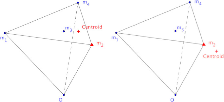
During the execution of the above algorithm, it is possible that many points from one point-set are assigned to the same cluster. Since at most one of them is allowed to appear in the final solution, we need to determine which small set of points to be kept in each iteration. Our idea is to shrink the trace of $W_{t}$ so that a peeling strategy can be adopted. Geometrically, we know that the set of (assigned) points from the same point-set uniquely define a convex cone. Our idea is to keep the points that are close to the centroid of the cluster and also on the boundary of the convex cone (i.e., the extreme points). The rationale behind this is that extreme points are more likely to be the closest points to other point-sets. By keeping such extreme points, we can better approximate the pairwise distances between different point-sets, which are needed to form clusters (see Fig. 2 for an example).

Figure 2.

Illustration of selecting the extreme points. The blue dots and red diamonds represent points from two different point-sets. The ‘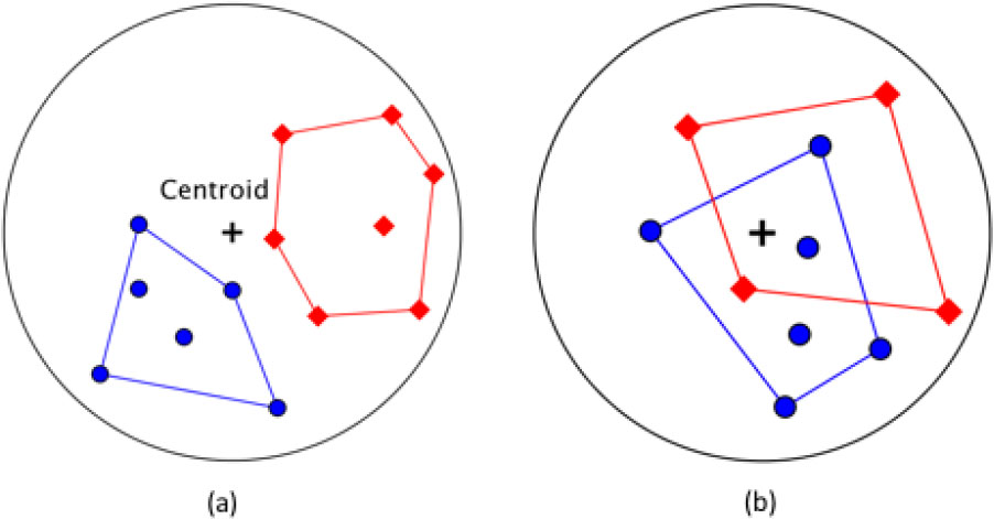 $+$ ’ is a centroid. The extreme points on the boundaries are good candidates of the representative points. $(a)$ shows the case that the centroid is outside of the convex cone and $(b)$ shows the inside case.

From a geometric point of view, trace minimization is equivalent to projecting the centroid to the convex cone formed by the extreme points. The projection is a non-negative linear combination (called features) of weighted extreme points. Hence an extreme point closer to the centroid tends to have a larger weight, meaning that it shares a larger portion of the common feature. There are two cases to consider based on the relative positions of a centroid with respect to the convex cone (see Fig. 3). The following theorems ensure the correctness.

Figure 3.

$\{m_{1},\ldots,m_{4}\}$ are points from a point-set assigned to the same cluster. The red ‘ $+$ ’ is the centroid and the red ‘ $\vartriangle$ ’ is the point with the largest weight $w_{jj}$ . The left and right figures show the inside and outside cases, respectively.

.

Let $M^{t}_{l}=[m^{t}_{1},m^{t}_{2},\ldots,m^{t}_{l_{t}}]$ be the $l_{t}$ points in point-set $M_{t}$ assigned to cluster $\pi_{l}$ . Let $\tilde{f}_{l}$ be the centroid locating in the convex cone of $M^{t}_{l}$ which has $r$ extreme points $M^{t}_{R}=[m^{t}_{1},\ldots,m^{t}_{r}]$ . Assume that there exists an extreme point $m^{t}_{p}\in M^{t}_{R}$ with $p\in[r]$ such that, for a constant $\delta_{p}>0$ ,

$\displaystyle\|m^{t}_{p}-\tilde{f}_{l}\|_{2}^{2}\leqslant\delta^{2}_{p}.$ (29)

Let $w^{t}_{p}$ be the weight of $m^{t}_{p}$ corresponding to $\tilde{f}_{l}$ . Then there exists $\kappa^{t}_{l}>0$ , such that

$\displaystyle w^{t}_{p}\geqslant 1-\frac{\delta_{p}}{\kappa^{t}_{l}}.$ (30)

Proof..

Given the point $\tilde{f}_{l}$ inside the cone, there exists a $r$ -size non-negative vector $x$ , such that $\tilde{f}_{l}=M^{t}_{R}x$ .

$\displaystyle\quad\|m^{t}_{p}-\tilde{f}_{l}\|_{2}^{2}$ $\displaystyle=\|m^{t}_{p}-M^{t}_{R}x\|_{2}^{2}$ $\displaystyle=\left\|m^{t}_{p}-x_{p}m^{t}_{p}-\sum_{j\in[r]\backslash p}x_{j}m% ^{t}_{j}\right\|_{2}^{2}$ $\displaystyle=\left\|(1-x_{p})m^{t}_{p}-\sum_{j\in[r]\backslash p}x_{j}m^{t}_{% j}\right\|_{2}^{2}$ $\displaystyle=(1-x_{p})^{2}\left\|m^{t}_{p}-\sum_{j\in[r]\backslash p}\frac{x_% {j}}{1-x_{p}}m^{t}_{j}\right\|_{2}^{2}$ (31)

Since $m^{t}_{p}$ is an extreme point of this cone, $m^{t}_{p}$ can not be represented by a convex combination of other extreme points. Hence, there exists $\kappa^{t}_{l}>0$ such that

$\displaystyle\min\left\|m^{t}_{p}-\sum_{j\in[r]\backslash p}\frac{x_{j}}{1-x_{% p}}m^{t}_{j}\right\|_{2}\geqslant\kappa^{t}_{l},\forall p\in[r].$ (32)

Then we can have

$\displaystyle\delta^{2}_{p}\geqslant(1-x_{p})^{2}\left\|m^{t}_{p}-\sum_{j\in[r% ]\backslash p}\frac{x_{j}}{1-x_{p}}m^{t}_{j}\right\|_{2}^{2}$ (33) $\displaystyle\quad\geqslant(1-x_{p})^{2}(\kappa^{t}_{l})^{2}.$ (34)

Therefore $x_{p}\geqslant 1-\frac{\delta_{p}}{\kappa^{t}_{l}}$ , which infers the result. ∎

From the above theorem, we immediately have the following.

.

Let the convex cone of $M^{t}_{l}$ , the extreme points $M^{t}_{R}$ and $m^{t}_{p}$ be defined as in Theorem 3. If the centroid $\tilde{f}_{l}$ is outside of the convex cone, there exists a $\kappa^{t}_{l}>0$ such that the weight

$\displaystyle w^{t}_{p}\geqslant 1-\frac{2\delta_{p}}{\kappa^{t}_{l}}.$ (35)

Proof..

Define the projection point of $\tilde{f}_{l}$ in the cone as $m^{t}_{\pi_{l}}$ by

$\displaystyle m^{t}_{\pi_{l}}=\operatornamewithlimits{argmin}_{y}\|y-\tilde{f}% _{l}\|,$ (36)

where $y=M^{t}_{R}x$ with $x\in[0,1]^{r}$ .

We have $\|y-\tilde{f}_{l}\|_{2}<\|m^{t}_{p}-\tilde{f}_{l}\|_{2}$ , since otherwise $m^{t}_{p}$ will be the projection point. Therefore, we have

$\displaystyle\quad\|y-m^{t}_{p}\|_{2}$ $\displaystyle=\|y-\tilde{f}_{l}+\tilde{f}_{l}-m^{t}_{p}\|_{2}$ $\displaystyle\leqslant\|y-\tilde{f}_{l}\|_{2}+\|\tilde{f}_{l}-m^{t}_{p}\|_{2}$ $\displaystyle\leqslant 2\delta_{p}.$ (37)

We then obtain the result by Theorem 3. ∎

4. Algorithms

We solve the model Eq. (24) using an alternative minimization framework, which is presented in Algorithm 4. In each iteration, our algorithm first clusters all weighted points based on the current centroids. Then it calculates the weights of each point-set by the divide-and-conquer method discussed in the previous section. For each point-set, we try to shrink the number of points falling in (or assigned to) the same cluster, which is achieved by the peeling step. At the end of each iteration, we update the centroids by selecting the most likely points from each cluster, instead of directly using the entire set of points. All these steps will be described in details in the following subsections.

[h] : General Alternative Minimization Framework[1] Input: The original dataset $M$ , initialized weights $W^{(0)}$ , centroids $F^{(0)}$ , cluster labels $G^{(0)}$ , number of iterations $T$ . Output: Selected $n$ points $\mathcal{Z}$ and the corresponding cluster labels. Begin $i=0$ , $\mathcal{Z}=\varnothing$ ; $|\mathrm{diag}(W)|_{0}>n$ $\&$ $F$ not converged $\&$ $i\leq T$ Update $G^{(i+1)}$ by solving

$\displaystyle\operatornamewithlimits{argmin}_{G}\|MW^{(i)}-F^{(i)}G\|_{F}^{2},% GG^{\top}=I$ (38)

Update $W^{(i+1)}$ by the divide-and-conquer strategy Eq. (28) $W^{(i+1)}\leftarrow\text{Peeling}(W^{(i+1)})$ Update $F^{(i+1)}$ by solving

$\displaystyle\operatornamewithlimits{argmin}_{F}\|\textit{MW}^{(i+1)}-\textit{% FG}^{(i+1)}\|_{F}^{2},\ F\geqslant 0$ (39)

i = i+1

t = 1 : n $\mathcal{Z}\leftarrow\mathcal{Z}\bigcup\{\text{Index}(m^{t}_{j})|\max\limits_{% 1\leqslant j\leqslant\lambda}w^{t}_{jj}\}$

Peeling $G$ according to $\mathcal{Z}$ End

4.1 Initialization

A good initialization can effectively improve the quality of our clustering result. We first extract $r$ main features of each point-set, where $r\ll\lambda$ is a small constant. This is performed by applying a rank- $r$ NMF on each point-set $M_{t}$ . Then, for each point-set, we find one feature $\psi_{i}$ shared by the most number of other point-sets. Since $r n$ is a small number, we can afford to search globally using pairwise distances. With this, we can generate good initial centroids $\mathcal{C}=\{c_{1},\ldots,c_{k}\}$ by applying $k$ -means clustering on these selected common features. We can also further update $\mathcal{C}$ by using the local search strategy in [9], which is presented in Algorithm 4.1. With the obtained centroids, we can compute the initial weight matrix $W^{(0)}_{t}$ for $M_{t}$ by the following equation, when features of $M_{t}$ are assigned to $\pi_{l}$ .

$\displaystyle w^{t}_{jj}=1-\frac{\|m_{j}^{t}-c_{l}\|_{2}}{\sum_{i=1}^{\lambda}% \|m_{i}^{t}-c_{l}\|_{2}},\ w^{t}_{ij}=0.$ (40)

Finally, we initialize $G^{(0)}$ using Eq. (38) with a necessary permutation. Note that if domain knowledge is given, it could be applied in generating the initial centroids. This would improve the quality of initial centroids, since the precision of sampling and searching in the the dataset increases, as long as the domain pre-knowledge is close to the true distribution of dataset.

: Local Search [9][1] Input: the initial $k$ centroids $\mathcal{C}^{0}=\{c^{0}_{1},\ldots,c^{0}_{k}\}$ , data matrix $M$ Output: $k$ centroids $\mathcal{C}=\{c_{1},\ldots,c_{k}\}$ Begin Calculate $D(m_{j})$ : the shortest distance from $m_{j}\in M$ to its closest centroid each point set $t=1:n$ In $M_{t}$ , choose $m^{t}_{j}$ has the $\min\limits_{j}D(m^{t}_{j})$ Update $\mathcal{C}$ by Kmeans $++$ on $n$ selected points $\{m^{t}_{j}\}_{t=1}^{n}$ $\mathcal{C}$ not converge Repeat the step 3 to 7 End [h] : Initialization[1] Input: original dataset $M$ Output: the initial centroids $\mathcal{C}$ Begin $\text{Fea}\in\mathbb{R}^{d\times rn}_{+}$ $\leftarrow$ rank- $r$ NMF on $M_{t}$ , $1\leqslant t\leqslant n$ $\Psi=\{\psi_{1},\ldots,\psi_{n}\}\in\mathbb{R}^{d\times n}_{+}\leftarrow\text{% Global search on Fea}$ Initial centroids $\mathcal{C}=\{c_{1},\ldots,c_{k}\}\leftarrow\mathrm{kmeans}(\Psi)$ (Optional) Update $\mathcal{C}$ via local search[9]. End

4.2 Non-negative least square methods for

G

To obtain $G$ , we use the efficient projected gradient method proposed in [21]. The main feature of this gradient method is that the orthogonality is enforced to $G$ by a projection onto the feasible set of the orthogonal matrices, known as the Stiefel manifold.

[h] : The peeling of $W$ [1] Begin $\mathcal{Q}=\varnothing$ each point set $t=1:n$ each cluster $\pi_{l},\ l=1:k$ $W_{t}^{l}$ : the corresponding weights of $M^{t}$ in $\pi_{l}$ $|\text{diag}(W_{t}^{l})|_{0}>1$ $j\leftarrow\operatornamewithlimits{argmin}_{j}w^{t}_{jj}$ or $\{j|w^{t}_{jj}\leqslant\theta\}$ $\mathcal{Q}\leftarrow\mathcal{Q}\bigcup\text{Index}(m^{t}_{j})$ Peel out the point $m_{j}$ if $j\in\mathcal{Q}$ End

4.3 Non-negative least square methods for $W$

We use the non-negative coordinate descent (NCD) method to solve Eq. (28). Coordinate descent method [30, 31] is a popular and efficient gradient method for solving NMF and NLS problems, which updates one variable of the unknown vector at a time.

In fact, when fixing all variables but a single entry $w^{t}_{pj}$ , we can write the Lagrangian form of Eq. (28) as a function of $w^{t}_{pj}$ :

$\displaystyle\quad\text{L}(w^{t}_{pj},\alpha,\beta)$ $\displaystyle=\|\textit{FG}_{t}-M_{t}W_{t}\|_{F}^{2}+\alpha q_{t}^{\top}\text{% diag}(W_{t})$ $\displaystyle\quad+\beta(\text{Tr}(W_{t})-1),$ $\displaystyle=\sum_{j=1}^{\lambda}\left\|\tilde{F}^{t}_{j}-\sum_{i=1}^{\lambda% }m^{t}_{j}w^{t}_{ij}\right\|_{2}^{2}+\alpha\sum_{j=1}^{\lambda}q^{t}_{j}w_{jj}% ^{t}$ $\displaystyle\quad+\sum_{j=1}^{\lambda}\beta(w^{t}_{jj}-1/\lambda),\ \ (% \mathrm{let}\ \tilde{F}^{t}=\textit{FG}_{t}),$ $\displaystyle=\sum_{j=1}^{\lambda}\left(\left\|\left(\tilde{F}^{t}_{j}-\sum_{i% \in[\lambda]\backslash p}m^{t}_{j}w^{t}_{ij}\right)-m^{t}_{p}w^{t}_{pj}\right% \|_{2}^{2}+\alpha q^{t}_{j}w_{jj}^{t}+\beta(w^{t}_{jj}-1/\lambda)\!\!\right) .$ (41)

Then NCD updates $w^{t}_{pj}$ by the following equation.

$\displaystyle w^{t}_{pj}\leftarrow w^{t}_{pj}+s\frac{\partial\text{L}(w^{t}_{% pj},\alpha,\beta)}{\partial w^{t}_{pj}}.$ (42)

Finally, we need to project $W_{t}$ onto the set $\{A|A\geqslant 0,\text{diag}(A)\leqslant 1,a_{ij}\leqslant a_{jj},\forall i,j\}$ . The projection is simple and can be done by using the method in [28].

4.4 Peeling strategy for

W

The numerical operations will be computationally expensive if we directly use the entire $N\times N$ weight matrix $W$ in the alternative minimization approach. The diagonal entries of $W$ is designed to indicate the possibility of the corresponding point being a representative point. As shown in Section 3.3, the trace of $W_{t}$ will gradually concentrate to one diagonal entry. Therefore, we can ignore the points with weights smaller than a certain threshold $\theta$ as shown in Algorithm 4.2.

To preserve the possibilities that a point-set may be clustered into different clusters, our algorithm allows each point-set to have multiple points assigned to different clusters during its execution (one for each at the end). In the final solution, it decides for each point-set its cluster by using the cluster label of the largest-weighted point.

4.5 Update the centroids $F$

We present an efficient and novel gradient descent method for updating the centroids. In the alternative minimization framework, $F$ is updated by solving the following NLS problem.

$\displaystyle\operatornamewithlimits{argmin}_{F}\|\textit{MW}-\textit{FG}\|_{F% }^{2},F\geqslant 0,$ (43)

with $W$ and $G$ fixed.

Now let $\tilde{M}=MW$ . By a simil ar deduction as for Eq. (2.2), we have

$\displaystyle\quad\operatornamewithlimits{argmin}_{F}\|\tilde{M}-FG\|_{F}^{2}$ $\displaystyle=\operatornamewithlimits{argmin}_{F}\sum_{j=1}^{N}\|\tilde{m}_{j}% -Fg_{j}\|_{2}^{2}$ $\displaystyle=\operatornamewithlimits{argmin}_{F}\sum_{l=1}^{k}\sum_{j\in\pi_{% l}}\|\tilde{m}_{j}-f_{l}g_{lj}\|_{2}^{2}$ $\displaystyle=\sum_{j\in[N]}\operatornamewithlimits{argmin}_{f_{l}}\sum_{l=1}^% {k}\|\tilde{m}_{j}-f_{l}g_{lj}\|_{2}^{2}.$ (44)

Then the gradient of Eq. (44) can be written as

$\displaystyle\frac{\partial\|\tilde{M}-\textit{FG}\|_{F}^{2}}{\partial F}=-2% \sum_{j=1}^{N}(\tilde{m}_{j}-Fg_{j})g_{j}^{\top}.$ (45)

Directly using this gradient will lead to a large computation burden, especially when $N$ is large (e.g., in large-scale datasets). Since the optimal $F^{\star}$ is decided by $n$ points, it is reasonable for us to only consider the points with large weights $w_{jj}$ ’s. Then in each iteration, we can update $F$ using the following new gradient

$\displaystyle\frac{\partial\|\tilde{M}-FG\|_{F}^{2}}{\partial F}=-2\sum_{j\in% \Omega}\left((\tilde{m}_{j}-Fg_{j})g_{j}^{\top}\right),$ (46)

where $\Omega=\cup^{n}_{i=1}\Omega_{i}$ . For each point set $M_{t}$ , $\Omega_{t}$ contains the indexes of the largest-weighted points from all its assigned clusters.

5. Experiments

In this section, we present the experimental results of our method on several benchmark clustering datasets.

5.1 The CBCL face database

The CBCL database [32] contains 2429 19 $\times$ 19 gray-scale PGM-format human faces. To illustrate the effectiveness of our method, we create point-sets by mixing images focusing on different features.

We firstly apply a normal NMF method to decompose each image into a combination of 20 features. Then we select 3 specific features as the centroids of 3 clusters, as shown in Fig. 4.

To construct the cluster of each selected feature, we randomly sample 60 images which are mainly represented by this feature. Following this, we manually vary the weights of this feature in these images, such that 10 of them have relatively larger weights. The distances of the images to its centroids are proportional to these weights. This is illustrated in Fig. 5.

Table 1
Accuracy results on synthetic CBCL face data

Method	UKmeans	SDP	ONMF	Kmeans $++$
Accuracy	96.67%	98.33%	56.67%	31.67%

Figure 4.

The selected 3 features (b) from a total 20 features (a) obtained by NMF on CBCL data.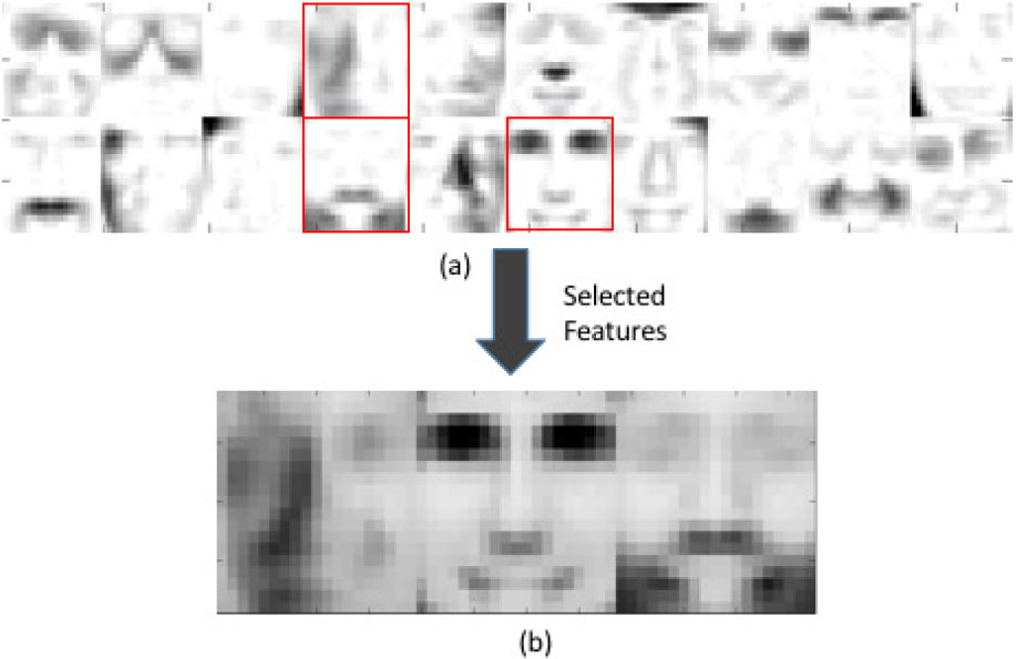

Figure 5.

An example of two clusters consist of images with different weights.

Now we construct 6 point-sets, each of which contains 30 images. A point-set is constructed by randomly mixing the large-weight images with the small-weight ones having different features. The cluster label of this point set is decided by the largest-weighted feature of its images. In this way, we can design the optimal solution by distributing the large-weight images of each cluster into different point-sets. We call them the representative images (points). An example is illustrated in Fig. 6. Therefore the quality of our clustering method can be measured by the representative images detected, since only one point is allowed to be kept in each point-set in the final solution.

Figure 6.

An example of 4 point-sets consisting of mixing images. Set $A$ and $B$ belong to Cluster $A$ . Set $C$ and $D$ belong to Cluster $B$ . In each point-set, the representative images (containing the largest-weighted feature) are isolated by red.

We construct the ground truth of our experiment as follows. Point-set 1 and 2 are labeled by representative images from cluster 1; point-set 3 and 4 are labeled by representative images from cluster 2; point-set 5 and $6$ are labeled by representative images from cluster 3. The result of our method is presented in Fig. 7, which shows that our method can successfully detect the representative images and hence obtain the correct clustering.

Figure 7.

The result of our method on synthetic data. An optimal solution is obtained in this experiment. The representative point in each point-set is showed in this figure and matches the corresponding features.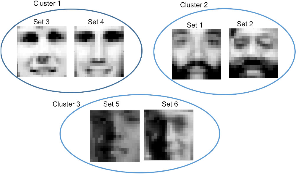

We compare the accuracy of our method with different methods: orthogonal NMF (ONMF) [21], Kmeans $++$ , and SDP model [9]. The ONMF and Kmeans $++$ are performed as the local search manner as in [9]. The experiment is taken on the datasets constructed as above and is respectively repeated 10 times for each method. The optimal solution should have a total of 60 representative images during 10 experiments. The accuracy is measured by the ratio of the number of detected representative images to the optimal number. The result is presented in Table 1. Our accuracy is very close to the best existing SDP method. However, our method has a much better running time than SDP.

We compare the running time of our method and that of the SDP model in Fig. 8, which clearly shows an outperforming advantage of our method in efficiency. The experiment is performed using the similar construction of point-sets and clusters, but with varying sizes. We choose 3 different sizes for each point-set: 15, 25 and 35. The corresponding total number of images is respectively 90, 150 and 210.

5.2 The USPS handwritten digit database

We also provide the comparison result on the USPS handwritten digit database [33], which contains 9298 16 $\times$ 16 handwritten digit images of numbers from 0 to 9.

We also construct the optimal representative images as in last experiment. But we do not manually affect each image. Every data point is an original image. In the experiment, we randomly select the images of the number 3, 2, 4 as the representative numbers to label the point-sets. Each point-set contains 30 images, constructed by mixing images of one representative number and images randomly selected from other different numbers. We have 6 point-sets and 3 clusters. An example is shown in Fig. 9.

Table 2
Accuracy comparison on real handwritten data

Method	UKmeans	SDP	ONMF	Kmeans $++$
Accuracy	85.00%	75.00%	33.33%	45.00%

Figure 8.

The efficiency comparison of UKmeans and SDP model.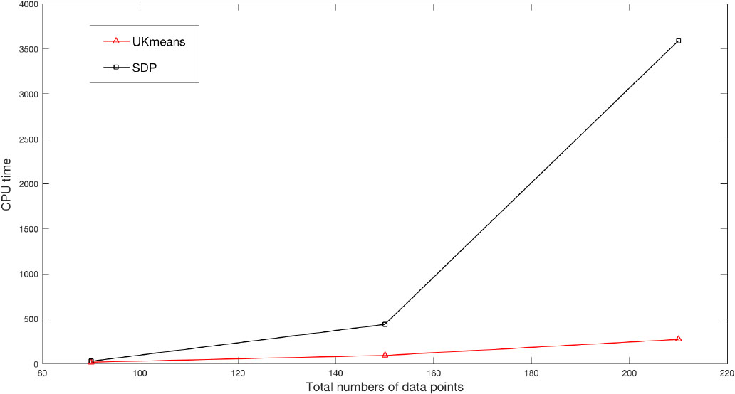

Figure 9.

An example of 2 point-sets consisting of mixing number images. Set 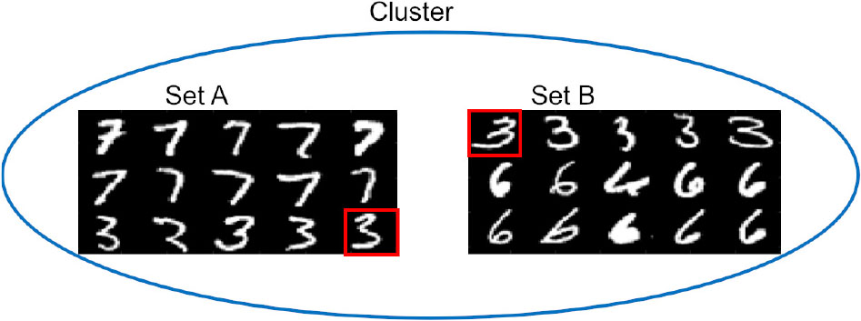$A$ and $B$ belong to the same cluster, since they both contain number 3.

The accuracy comparisons are provided in Table 2, which are conducted in the same manner as for the face data. The real handwritten data is much easier to be confused with each other. This is because no fixed handwritten type exists for each number. For instance, 2 may be written similarly as 7, and 4 could be close to 6 and 9. Also Euclidean distance is not very suitable for measuring the similarity, since the $l_{2}$ norm of a image depends on the handwritten style. This leads to a decrease in accuracy for each method. Our method has the highest accuracy as expected, since it compares the features instead of Euclidean distances. This confirms the effectiveness of our model.

5.3 2-D Gaussian data

Figure 10.

The D $28$ data set is generated as 28 similar 2-D Gaussian distributions.

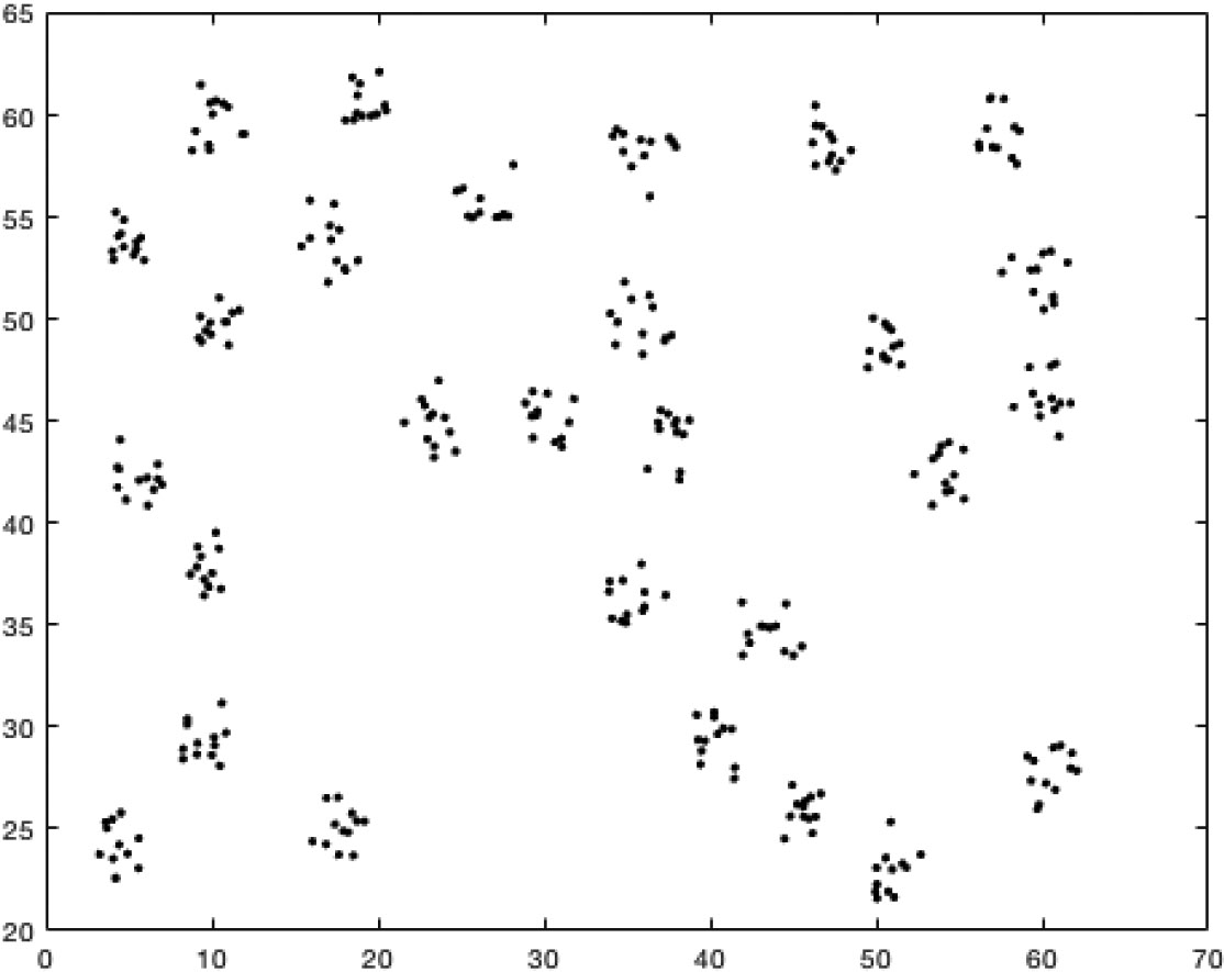
In this subsection, we demonstrate the effectiveness of our method by providing the comparison results on the random D28 data set [4], which consisting of 28 similar 2-D Gaussian distributions as in Fig. 10. In this data set, there are total 336 points, with each Gaussian distribution contains 12 points.

The core difference between the Gaussian data and the previous face data is that the Gaussian data set purely contains geometric information. In this scenario, the clustering result depends more on the relative geometric locations than the features of data points, since the features (extreme points) of each Gaussian distribution are not unique.

Now we partition this data set into 12 uncertain point sets such that each point set has 28 points. The uncertain clustering will group different point sets into one cluster based on the smallest $l_{2}$ pairwise distance within points. There are 4 clusters designed for these uncertain point sets. We construct the ground truth for this experiment in a similar manner as the previous experiments. Firstly, we randomly select 4 Gaussian distributions to label the 4 clusters, noted as label sets. We uniformly divide each label set into 3 parts, with 4 points in each part. Then we create each uncertain point set by randomly choosing 2 Gaussian distributions from the data set and 4 representative points from one label set. In this way, 3 point sets are grouped into one cluster as long as they contain the points from the same label set. This construction is illustrated in Fig. 11.

Figure 11.

An example of 3 point-sets falling into one cluster. Set 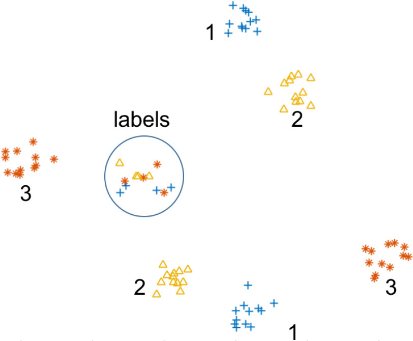$1,2$ and 3 belong to the same cluster, since they all contain points from the same label set.

Figure 12.

ARI comparisons on Gaussian dataset.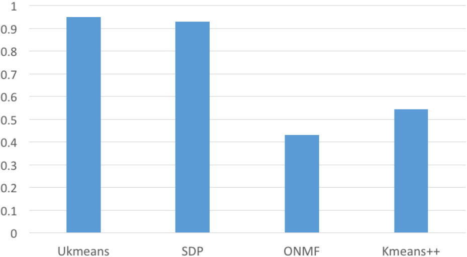

Figure 13.

72 cities forms 9 clusters with 8 points in one cluster. And ‘ $+$ ’ indicates the mean point of one cluster.

The accuracy of clustering is displayed by the Adjusted Rand Index (ARI) [34]. The comparisons are provided in Fig. 12, which are conducted in the same manner as for the face data. This result demonstrates our method is effective for the data with less feature information. The accuracy of our method is better than the state-of-art SDP method. The reason is that each Gaussian distribution in the original data set is tight and separated from other distributions. The extreme points of each point set can be easily calculated and precisely matched the boundary of the point set. Hence it is desirable for our method to locate the label points.

5.4 City distance dataset

Here we present our comparison results on a real data set, which contains the 2-D coordinates of 72 cities in North America [35]. The construction of uncertain data sets is similar as the processing of the Gaussian data. To construct the ground truth, we firstly apply Kmeans on the 72 cities to obtain 9 clusters, which can be shown in Fig. 13.

We partition this data set into 6 uncertain point sets such that each point set contains 12 points (one city cluster and 4 label points). These uncertain point sets are designed to form 3 clusters. Each cluster is labeled by one randomly chosen city cluster, as in Fig. 14.

Figure 14.

The illustration of 3 clusters formed by 6 uncertain point sets. Each point set is colored by a unique color.

We present the ARI results of clustering in Fig. 15. Our method achieves a slightly lower accuracy than the SDP method. This is because the real city data points spreads more randomly in the space. And the city clusters are not tight as the previous Gaussian clusters. However, the speed of our method largely outperforms the state-of-art SDP method, which has been demonstrated in the previous example. And the results of real data strongly confirms the ability of our method in practical area.

Figure 15.

ARI comparisons on city distance dataset.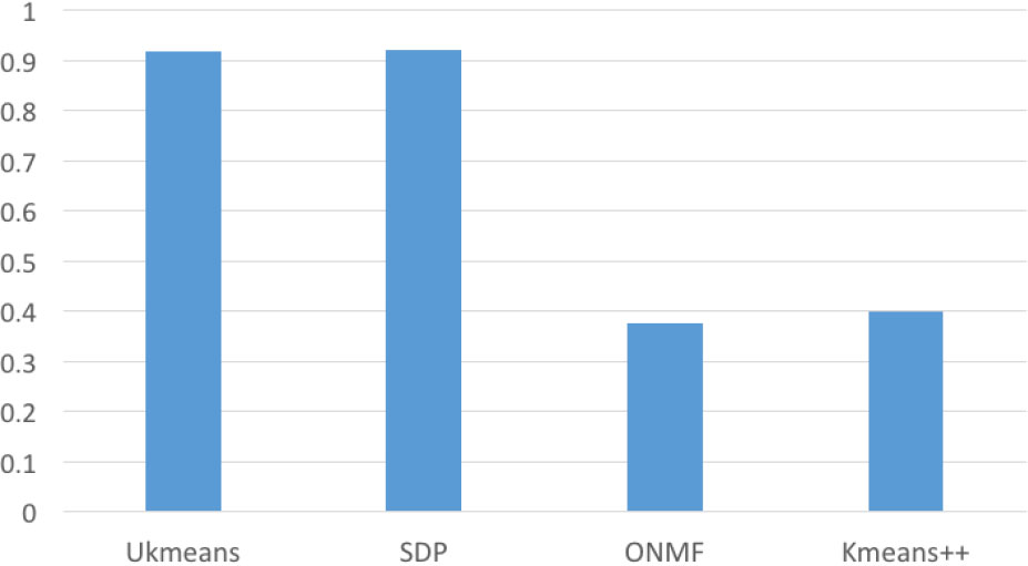

6. Conclusion

In this paper, we considered the problem of clustering uncertain data, and designed a new feature-based strategy to locate the representative point among a set of possible points. By introducing a novel NMF model, we can successfully avoid the expensive SDP computation on the whole dataset. The correctness of our model is proved by the provided theoretical analysis, and efficient computation strategies are designed in our algorithm. Experiments on benchmark datasets strongly support the effectiveness and efficiency of our method.

Footnotes

Acknowledgments

This work is supported in part by the National Natural Science Foundation of China under Grant No. 5187492 and Guangxi University’s High-level Talents Start-up Found under Grant No. A3070051002.

References

Andreetto

Zelnik-Manor

and Perona

, Non-parametric probabilistic image segmentation, in: Computer Vision, 2007. ICCV 2007, IEEE, 2007, pp. 1–8.

Zass

and Shashua

, A unifying approach to hard and probabilistic clustering, in: Computer Vision, 2005. ICCV 2005, Vol. 1, IEEE, 2005, pp. 294–301.

Sun

Cheng

Cheung

D.W.

and Cheng

, Mining uncertain data with probabilistic guarantees, in: Proceedings of the 16th ACM SIGKDD, ACM, 2010, pp. 273–282.

Züfle

Emrich

Schmid

K.A.

Mamoulis

Zimek

and Renz

, Representative clustering of uncertain data, in: Proceedings of the 20th ACM SIGKDD, ACM, 2014, pp. 243–252.

Ngai

W.K.

Kao

Chui

C.K.

Cheng

Chau

and Yip

K.Y.

, Efficient clustering of uncertain data, in: Data Mining, 2006. ICDM’06, IEEE, 2006, pp. 436–445.

Günnemann

Kremer

and Seidl

, Subspace clustering for uncertain data, in: Proceedings of the 2010 SIAM ICDM, SIAM, 2010, pp. 385–396.

Lammersen

Schmidt

and Sohler

, Probabilistic k-median clustering in data streams, Theory of Computing Systems 56(1) (2015), 251–290.

Ding

Stojkovic

Berezney

and Xu

, Gauging association patterns of chromosome territories via chromatic median, in: Proceedings of the IEEE CVPR, 2013, pp. 1296–1303.

Chen

Ding

Chen

Wang

Fritz

Sehgal

Berezney

and Xu

, Mining k-median chromosome association graphs from a population of heterogeneous cells, in: Proceedings of the 6th ACM BCB, ACM, 2015, pp. 47–56.

10.

Aggarwal

C.C.

and Philip

S.Y.

, A survey of uncertain data algorithms and applications, IEEE Transactions on Knowledge and Data Engineering 21(5) (2009), 609–623.

11.

Chau

Cheng

Kao

and Ng

, Uncertain data mining: An example in clustering location data, in: Pacific-Asia Conference on Knowledge Discovery and Data Mining, Springer, 2006, pp. 199–204.

12.

Gullo

Ponti

and Tagarelli

, Clustering uncertain data via k-medoids, in: International Conference on Scalable Uncertainty Management, Springer, 2008, pp. 229–242.

13.

Cormode

and McGregor

, Approximation algorithms for clustering uncertain data, in: Proceedings of the twenty-seventh ACM SIGMOD-SIGACT-SIGART, ACM, 2008, pp. 191–200.

14.

Guha

and Munagala

, Exceeding expectations and clustering uncertain data, in: Proceedings of the twenty-eighth ACM SIGMOD-SIGACT-SIGART, ACM, 2009, pp. 269–278.

15.

Ding

and Xu

, A unified framework for clustering constrained data without locality property, in: Proceedings of the Twenty-Sixth Annual ACM-SIAM SODA, Society for Industrial and Applied Mathematics, 2015, pp. 1471–1490.

16.

Donoho

and Stodden

, When does non-negative matrix factorization give a correct decomposition into parts? in: NIPS, 2003, pp. 1141–1148.

17.

Chen

Wang

and Zhang

, Collaborative filtering using orthogonal nonnegative matrix tri-factorization, Information Processing & Management 45(3) (2009), 368–379.

18.

Kim

Chen

Kim

Pan

and Park

, Sparse nonnegative matrix factorization for protein sequence motif discovery, Expert Systems with Applications 38(10) (2011), 13198–13207.

19.

Lee

D.D.

and Seung

H.S.

, Learning the parts of objects by non-negative matrix factorization, Nature 401(6755) (1999), 788–791.

20.

Zha

Ding

and Simon

H.D.

, Spectral relaxation for k-means clustering, in: NIPS, 2001, pp. 1057–1064.

21.

Pompili

Gillis

Absil

P.-A.

and Glineur

, Two algorithms for orthogonal nonnegative matrix factorization with application to clustering, Neurocomputing 141 (2014), 15–25.

22.

Ding

C.H.

and Simon

H.D.

, On the Equivalence of Nonnegative Matrix Factorization and Spectral Clustering, in: SDM, Vol. 5, SIAM, 2005, pp. 606–610.

23.

Gegick

, Symmetric nonnegative matrix factorization for graph clustering (2012).

24.

Ding

Peng

and Park

, Orthogonal nonnegative matrix t-factorizations for clustering, in: Proceedings of the 12th ACM SIGKDD, ACM, 2006, pp. 126–135.

25.

Ding

C.H.

and Jordan

M.I.

, Convex and semi-nonnegative matrix factorizations, PAMI 32(1) (2010), 45–55.

26.

Kim

and Park

, Sparse nonnegative matrix factorization for clustering (2008).

27.

Inaba

Katoh

and Imai

, Applications of weighted Voronoi diagrams and randomization to variance-based k-clustering, in: Proceedings of the tenth annual symposium on Computational geometry, ACM, 1994, pp. 332–339.

28.

Recht

Tropp

and Bittorf

, Factoring nonnegative matrices with linear programs, in: Advances in Neural Information Processing Systems, 2012, pp. 1214–1222.

29.

Gillis

and Luce

, Robust near-separable nonnegative matrix factorization using linear optimization., Journal of Machine Learning Research 15(1) (2014), 1249–1280.

30.

Gillis

and Glineur

, Accelerated multiplicative updates and hierarchical ALS algorithms for nonnegative matrix factorization, Neural computation 24(4) (2012), 1085–1105.

31.

Hsieh

C.-J.

and Dhillon

I.S.

, Fast coordinate descent methods with variable selection for non-negative matrix factorization, in: Proceedings of the 17th ACM SIGKDD, ACM, 2011, pp. 1064–1072.

32.

Alvira

and Rifkin

, An Empirical Comparison of SNoW and SVMs for Face Detection, A.I. memo, 2001–004, Center for Biological and Computational Learning, MIT, Cambridge, MA, 2001.

33.

Cai

Han

and Huang

T.S.

, Graph regularized nonnegative matrix factorization for data representation, IEEE Transactions on Pattern Analysis and Machine Intelligence 33(8) (2011), 1548–1560.

34.

Hubert

and Arabie

, Comparing partitions, Journal of Classification 2(1) (1985), 193–218.

35.

Burkardt

, CITIES dataset. https://people.sc.fsu.edu/∼jburkardt/datasets/cities/cities.html.

36.

Woodruff

D.P.

, Sketching as a tool for numerical linear algebra, arXiv preprint arXiv:1411.4357 (2014).

37.

Tjioe

Berry

Homayouni

and Heinrich

, Using a literature-based NMF model for discovering gene functional relationships, BMC Bioinformatics 9(7) (2008), 1.

38.

Hofmann

, Probabilistic latent semantic indexing, in: Proceedings of the 22nd annual international ACM SIGIR, ACM, 1999, pp. 50–57.

39.

Guillamet

and Vitria

, Non-negative matrix factorization for face recognition, in: Topics in artificial intelligence, Springer, 2002, pp. 336–344.

40.

Potluru

V.K.

Plis

S.M.

Roux

J.L.

Pearlmutter

B.A.

Calhoun

V.D.

and Hayes

T.P.

, Block coordinate descent for sparse NMF, arXiv preprint arXiv:1301.3527 (2013).

41.

Hartigan

J.A.

and Wong

M.A.

, Algorithm AS 136: A k-means clustering algorithm, Journal of the Royal Statistical Society. Series C (Applied Statistics) 28(1) (1979), 100–108.

42.

Dalvi

and Suciu

, Efficient query evaluation on probabilistic databases, The VLDB Journal 16(4) (2007), 523–544.

43.

Cheng

Kalashnikov

D.V.

and Prabhakar

, Querying imprecise data in moving object environments, IEEE Transactions on Knowledge and Data Engineering 16(9) (2004), 1112–1127.

44.

Deshpande

Guestrin

Madden

S.R.

Hellerstein

J.M.

and Hong

, Model-based approximate querying in sensor networks, The VLDB Journal 14(4) (2005), 417–443.

45.

Tao

Cheng

Xiao

Ngai

W.K.

Kao

and Prabhakar

, Indexing multi-dimensional uncertain data with arbitrary probability density functions, in: Proceedings of the 31st international conference on Very large data bases, VLDB Endowment, 2005, pp. 922–933.

46.

Gullo

and Tagarelli

, Uncertain centroid based partitional clustering of uncertain data, Proceedings of the VLDB Endowment 5(7) (2012), 610–621.

47.

Yang

and Oja

, Linear and nonlinear projective nonnegative matrix factorization, IEEE Transactions on Neural Networks 21(5) (2010), 734–749.

48.

Choi

, Algorithms for orthogonal nonnegative matrix factorization, in: Neural Networks, 2008. IJCNN 2008, IEEE, 2008, pp. 1828–1832.

Sparse non-negative matrix factorization for uncertain data clustering

Abstract

Keywords

1. Introduction

2.1 Related results on uncertain clustering

2.2 Related results on NMF-based clustering

3.1 Problem definition

.

.

Proof..

.

.

Proof..

Proof..

.

Proof..

.

Proof..

4.3 Non-negative least square methods for W

4.5 Update the centroids F

5.1 The CBCL face database

Table 1 Accuracy results on synthetic CBCL face data

Table 2 Accuracy comparison on real handwritten data

Footnotes

Acknowledgments

References

4.3 Non-negative least square methods for $W$

4.5 Update the centroids $F$

Table 1
Accuracy results on synthetic CBCL face data

Table 2
Accuracy comparison on real handwritten data