
Abstract
Recommender systems apply machine learning and data mining techniques for filtering unseen information, and they can provide an opportunity to predict whether a user would be interested in a given item. The main types of recommender systems are collaborative filtering (CF) and content-based filtering, which suffer from scalability and data sparsity resulting in poor quality recommendations and reduced coverage. There are two incremental algorithms based on Singular Value Decomposition (SVD) with high scalability for recommender systems which are named the incremental SVD algorithm and incremental Approximating the Singular Value Decomposition (ApproSVD) algorithm. In both mentioned methods, the estimated value of rank for approximating the recommender systems’ data matrix is chosen experimentally in the related literature. In this paper, we investigate the role of singular values for estimating a more reliable amount of rank in the mentioned dimensionality reduction techniques to improve the recommender systems’ performance. In other words, we offered a strategy for choosing the optimal rank that approximates the data matrix more accurately in incremental algorithms with the help of singular values. The numerical results illustrate that the suggested strategy improves the accuracy of the recommendations and run times of both algorithms when employs for Movielens, Netflix, and Jester dataset.
Keywords
Introduction
Related works
Recommender Systems are software tools and techniques for assisting in the prediction of the users’ opinion to suggest to them the most appropriate item of interest. The aim is to support users in various decision-making processes, such as what items to buy, what news to read, or what music to listen. Recommender systems rely on different types of input data, which are often placed in a matrix with one dimension representing users and the other dimension representing items, which includes explicit input by users regarding their interest in products. We refer to explicit user feedback as ratings. Usually, explicit feedback composes a sparse matrix, due to the fact that there is the possibility of some users have rated only a small range of items.
Recommender systems are valuable means for on-line users to cope with information overload. During the last decade, various techniques for generating recommendations have been proposed, and many of them have been successfully spread in commercial environments. That is why recommender systems have become one of the most powerful and popular tools in electronic commerce. There are two main types of recommender systems: collaborative filtering (CF) and content-based filtering. The principle of collaborative filtering is to recommend the active user the items that other users with similar tastes liked in the past. The similarity in the taste of two users is calculated based on the similarity in the rating history. The common challenge of collaborative filtering and other types of recommender systems is dealing with massive data and sparsity to make accurate recommendations. Hence, the size of a dataset and its information sufficiency should be concidered to make accurate predictions efficiently. In addition, data arrives in no particular order as new rows and columns. The existing and new data may be added, changed, or retracted in any order. The ultimate size of the data matrix is unknown. The collected data will typically be very sparse, but missing values cannot be presumed to be zeros. Several approaches have been proposed to remedy the sparsity and scalability problems associated with the CF, such as supervised classification techniques [2], unsupervised clustering techniques [13], and dimensionality reduction approaches, which include many methods such as singular value decomposition [18], low-rank approximation using matrix factorization techniques [17, 10], and principal component analysis [8].
The use of SVD as a tool to improve collaborative filtering has been known for some time. It is a powerful technique for dimensionality reduction. The reduced orthogonal dimensions resulting from SVD are less noisy than the original data and keep the latent associations among the terms and documents. Earlier work took advantage of this semantic property to reduce the dimensionality of feature space [13]. The task is to compute the best running estimation of a rank-k SVD from the actual data matrix, without any storage or caching of incoming data, and make recommendations [3]. As Sarwar described in [15], one of the significant advantages of SVD is that there are incremental algorithms to compute an approximated decomposition. This allows accepting new users or ratings without having to recompute the model that had been built from previously existing data. The same idea was later extended and formalized by Brand [3] into an on-line SVD model. The use of incremental SVD methods has become a commonly accepted approach after its success in the Netflix Prize. In [14], Sarwar has introdused the incremental SVD algorithms, for recommender systems, but for determining the optimal value of rank
Contribution
Previous studies [14, 18, 19] have illustrated that incremental SVD-based algorithms are successful in accuracy and scalability, but in all researches the optimal value of the dimension reduction matrix
Organization
The rest of the paper is organized as follows: Some preliminaries associated with basic mathematics definitions have been described in the next section. Section 3 explores the incremental SVD-based algorithm and the primary strategy for choosing the optimal rank in the original data matrix. Finally, the numerical results of our research have been discussed in Section 4.
Preliminaries
Low-rank approximation
The Low-rank matrix approximation estimates a matrix by one whose rank is less than that of the original matrix. The aim is to compute more compact representations of the data with limited loss of information [9]. Let
It can be stored and manipulated more economically than the matrix itself. In the above approximation, only
Singular value decomposition (SVD) provides the true rank and gives the best low-rank approximation of a matrix, and it has vast applications in many areas [9]. The other successful method is Non-negative Matrix Factorization (NMF). NMF characterizes both items and users by vectors of factors inferred from item rating patterns in their basic form.. These methods have become popular in recent years by combining good scalability with predictive accuracy. They offer much flexibility for modeling various real-life situations.
Matrix completion
One strength of matrix factorization is that it allows the incorporation of additional information. When explicit ratings are not available, recommender systems can infer user preferences by using implicit ratings, which indirectly reflects their opinions by observing user’s behavior compared to other users’ search patterns or purchase history. High-rank matrix completion is the problem of (approximately) recovering a data matrix from very few observed entries. It has wide applications in machine learning, especially in on-line recommendation systems [4]. There are some sensible approaches for filling the missing values before applying the SVD, leading to a significant performance increase. Usually, the missing values in the user-item rating matrix are filled by zero. This approach is straightforward and efficient in computation, which makes it very common. However, this approach does not consider the data variance’s underlying correlation structure affecting the data variance, which is generally high. Subsequently, if we have a large number of missing values, this imputation approach can result in inaccurate recommendations. The list of other imputation methods includes filling the rating matrix by random numbers, normal distribution, uniform distribution, item or user average, SVM classifier, and so on [7]. In this paper, we applied user average instead of missing values in the data matrix before computing SVD decomposition.
Singular value decomposition (SVD)
The core of the SVD algorithm lies in the following theorem.
(Singular Value Decomposition (SVD)).
Let
where
The truncated SVD algorithm is used to compute a small number of singular values instead of calculating all the singular values of a matrix. By means of TSVD, we can calculate an approximation of a matrix using less data than the original matrix. In other words, If we discard all but the
Eckart-young theorem
(Eckart-Young [5]).
Let
where
.
SVD also gives the best low rank approximation in spectral norm:
Often the analyzing data is non-negative, and the low-rank data are further required to be comprised of non-negative values to avoid physical realities contradiction. Classical approaches cannot guarantee to keep the non-negativity. The method for finding reduced rank non-negative factors to approximate a given non-negative matrix is the so-called non-negative matrix factorization (NMF) problem which can be defined in general form as follows:
(NMF problem).
Let
where
Note that these two low-rank matrices’ dimension is vital in estimating the most optimal approximation of
Principal component analysis
In recent years, the amount of data that requires to be analyzed or stored has constantly been increasing. Fortunately, high-dimensional data can often be modeled as a low-dimensional subspace of the original dimension. Under this assumption, an approximate representation can be discovered via a principal component analysis (PCA). PCA is a way of identifying patterns in data and expressing them in such a way as to highlight their similarities and differences. Since patterns in data can be hard to find in high-dimension data, where the graphical representation is not available, PCA is a powerful tool for analyzing data. The other main advantage of PCA is that once the data patterns have been found, they can be compressed. In other words, the dimension of data can be reduced without much loss of information. PCA is almost the same as the SVD; however, before computing singular vectors, we have to subtract the mean from each row of
Incremental algorithms
A Recommender system consists of two primary entities: users
which
There are two separate steps in the performance of collaborative filtering (CF) type of recommender systems, the first step, which is called off-line or model building, is usually neighborhood formation or investigating the similarity of user-user or item-item, and the second step is the on-line or execution process, which the actual prediction production can be considered as the on-line step. If there is no great change in the rating matrix in a short period frequently, recommender systems may compute off-line steps once a day or a week. Researchers have shown that SVD-based dimensional reduction algorithms can estimate better the data matrix in the off-line step for finding similarities among the data [13, 15]. SVD-based models perform pretty excellent in the on-line step with a run time of
Besides being time-consuming, SVD requires complete data. In many experimental settings, some parts of the measurement matrix may be missing, contaminated, or untrusted, so imputation techniques are applied for overcoming these problems [6]. As we have mentioned in Section 2.2, we replaced the users’ average ratings instead of missing values, which were already filled by zeros, before the performance of SVD.
As we mentioned before, one of the significant challenges with data matrix in recommender systems is the time-consuming computation in the off-line procedure of incremental SVD-based algorithms. One of the solutions is reducing the dimension of the data matrix with factorization methods. Hence, we should find an appropriate method for computing the nearest rank to the original matrix in the algorithm. This strategy has been inspired by the choosing rule for SVD-NMF in [12] and assists us to find the most optimal amount of rank
Suppose
This idea is meaningful due to the fact that the non-zero elements of
Let the matrix
where
Now by considering optimal rank
Therefore, the SVD of
where
where
Notice that, the matrices
InputInput OutputOutput ReturnReturn Optimal incremental SVD algorithmmatrices
[b] InputInput OutputOutput ReturnReturn Optimal incremental ApproSVD algorithm
matrices
The
The ApproSVD approach has been suggested in [19], and incremental ApproSVD has been introduced in [18], which can solve the scalability challenge in a recommender system. In this method, the most important facet is choosing sampling probabilities of the data matrix’s columns and newly added matrix. Suppose that the chosen column sampling probabilities are
Experimental evaluation
This section describes the experimental validation of choosing optimal
Datasets
The first dataset for performing our experiments is the MovieLens dataset [20]. Each week, hundreds of users visit MovieLens to rate and receive recommendations for movies. The dataset can be converted into a user-item matrix with 943 rows (users) and 1682 columns (movies), in which approximately 6.3% of entries are filled. The sparsity of a dataset is calculated by
The second dataset is Netflix [21], and we just have performed our experiments on a small part of the dataset. It is a user-item matrix with 930 rows and 241 items, in which there are 1.5% of ratings. The Netflix data matrix has 3250 ratings, and like Movielens, the unrated items get zero values. The rating range is between 1 and 5, where 1 shows the lowest interest and 5 represents a strong interest.
Last but not least is the Jester dataset [22]. This data matrix is different from two other datasets, the ratings are between
Feature extraction and selection
First of all, we have tried to fill the sparse matrix by using imputation methods for Movielens and Netflix datasets. Thus the average amount of ratings in each row (user’s average imputation method) replaced instead of zeros in the same row of the data matrix. Then, rating the entries in the dataset is randomly divided into five partitions to execute five-fold cross validation. In other words, all ratings were evenly divided into five disjoint folds and applied four folds together to train our algorithm, and use the remaining fold as a test set to evaluate the performance. This process is repeated five times; therefore, we used each fold as a test set once. Algorithms performed on training data to make predictions for the test set. The data used to test the model is called the validation set, while the data used to create the model is called the training set. For each of these pairs, the model is trained on the training set and validated on the validation set.
The Mean Absolute Error (MAE) and Root Mean Squared Error (RMSE) are applied to measure the closeness of predicted ratings and genuine ratings as evaluation scales. Let
The computed values of MAE and RMSE demonstrate the accuracy of the algorithm.
All the experiments were executed in MATLAB R2017a, running on a Windows 8.1 with Intel Pentium Core i5 with 4GB RAM. For the Movielens dataset, as we are mainly comparing the results of our experiment with the numerical results in [18], we have considered the same numerical conditions in [18] for both algorithms while applying optimal rank
Tables 1 and 2 represent the amounts of MAE, RMSE, and running time of incremental SVD-based algorithms. Both tables are divided into two main parts for comparison. The first part of Tables 1 and 2 are related to numerical execution of optimal incremental SVD and optimal incremental ApproSVD, respectively. The second part of the tables is the numerical results in [18]. Therefore, we have chosen the same column size as [18] for presenting our strategy’s efficiency in choosing the most appropriate rank. In addition, the reason behind the larger amount of RMSE than MAE is that the calculated errors are squared before being summed in Eq. (8).
Comparing the performance of optimal incremental SVD and regular incremental SVD algorithms [18], by using Movielens dataset
Comparing the performance of optimal incremental SVD and regular incremental SVD algorithms [18], by using Movielens dataset
In Table 1, the first column is the column size of the original matrix
Comparing the performance of optimal incremental ApproSVD and regular incremental ApproSVD algorithms [18], by using Movielens dataset
In Table 2, for the first column, we considered
Table 3 includes the results of performing incremental SVD algorithm on Netflix dataset. We divided the table into three different parts: Optimal incremental SVD, regular incremental SVD with fixed rank
Experimenting optimal incremental SVD and regular incremental SVD algorithms (with fixed amount of rank
Experimenting optimal incremental SVD and regular incremental SVD algorithms (with fixed amount of rank
Table 5 illustrates the performance of incremental ApproSVD algorithms on the Netflix dataset. The table has three main parts, including the results in optimal incremental ApproSVD, regular incremental SVD with a fixed
Table 6 is the representation of applying ApproSVD on the Jester dataset with
Performance of optimal incremental ApproSVD and regular incremental ApproSVD algorithms (with fixed amount of
Numerical results of optimal incremental ApproSVD and regular incremental ApproSVD algorithms (with fixed amount of
MAE of optimal incremental SVD algorithm with the change of original column size on Movielens dataset.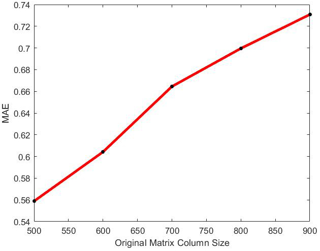
RMSE of optimal incremental SVD algorithm with the change of original column size on Movielens dataset.
MAE values of optimal incremental SVD algorithm with the change of k on Movielens dataset.
RMSE values of optimal incremental SVD algorithm with the change of k on Movielens dataset.
Running time of optimal incremental SVD with the change of original column size on Movielens dataset.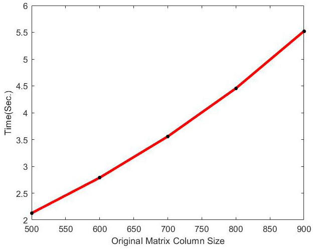
Running time of optimal incremental SVD algorithm with the change of k on Movielens dataset.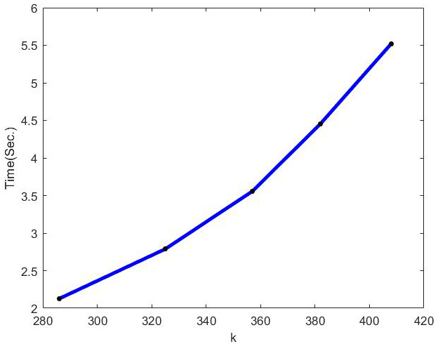
MAE of optimal incremental ApproSVD algorithms with the change of original column size on Movielens dataset.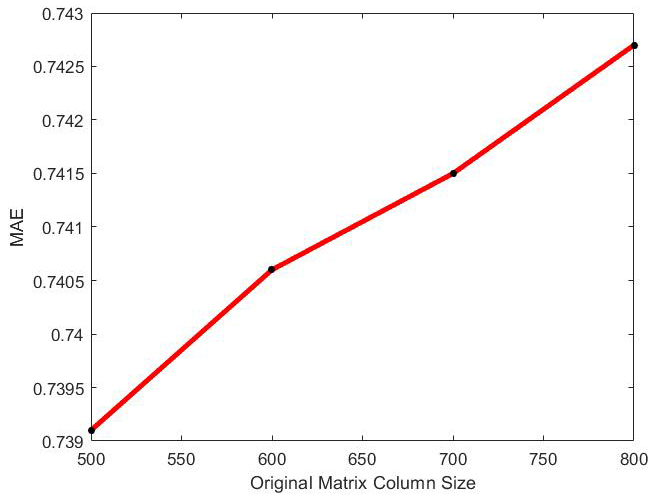
RMSE of optimal incremental ApproSVD algorithms with the change of original column size on Movielens dataset.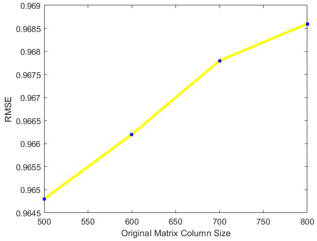
MAE values of optimal incremental ApproSVD algorithm with the change of k on Movielens dataset.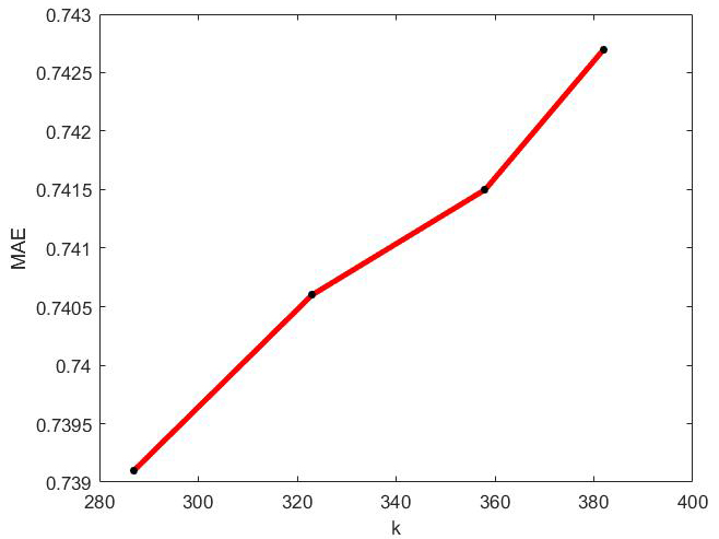
RMSE values of optimal incremental ApproSVD algorithm with the change of k on Movielens dataset.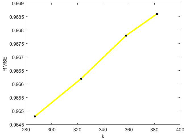
Running time of optimal incremental ApproSVD algorithm with the change of k on Movielens dataset.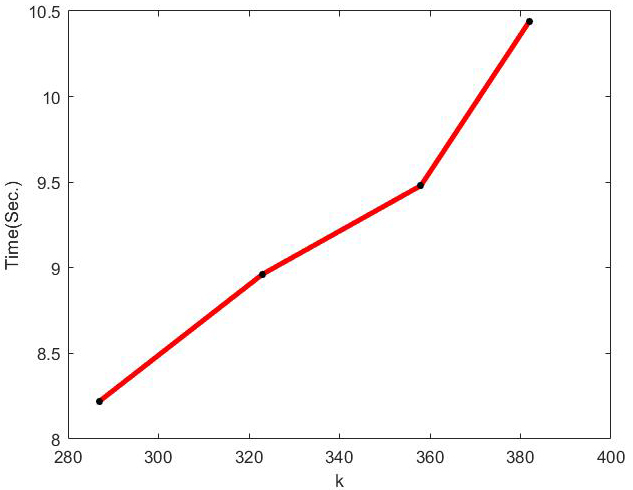
Running time of optimal incremental ApproSVD algorithms with the change of original column size on Movielens dataset.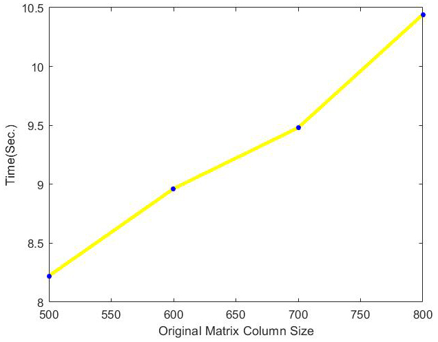
MAE values of optimal incremental SVD algorithm with the change of k on Jester dataset.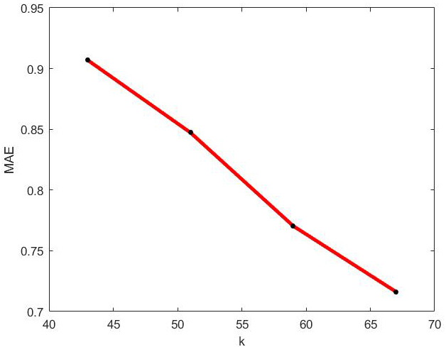
MAE values of optimal incremental SVD algorithm with the change of k on Netflix dataset.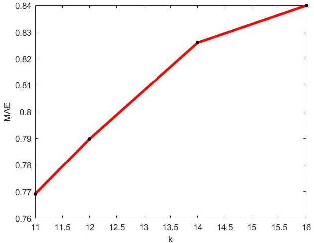
RMSE values of optimal incremental SVD algorithm with the change of k on Jester dataset.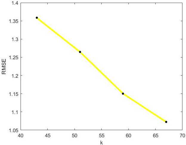
RMSE values of optimal incremental SVD algorithm with the change of k on Netflix dataset.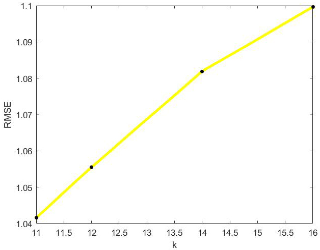
RMSE values of optimal incremental ApproSVD algorithm with the change of k on Jester dataset.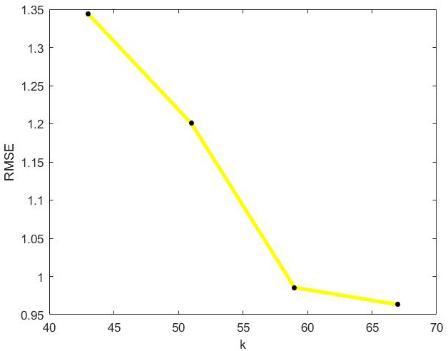
RMSE values of optimal incremental ApproSVD algorithm with the change of k on Netflix dataset.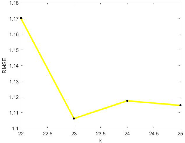
MAE values of optimal incremental ApproSVD algorithm with the change of k on Jester dataset.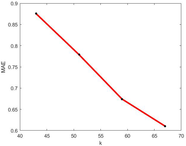
MAE values of optimal incremental ApproSVD algorithm with the change of k on Netflix dataset.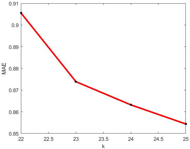
The behavior of optimal incremental SVD for Movielens dataset has been shown in Figs 1–6. According to Figs 1–4, the increase in amounts of original column size and
According to Figs 14 and 16, the amounts of MAE and RMSE in applying incremental SVD algorithm on Netflix dataset have increased by increasing the amount of rank
In this paper, we tried to apply a mathematical method for choosing a reliable optimal rank