Predicting remaining execution time of business process instances via auto-encoded transition system

Abstract

As an important task in business process management, remaining time prediction for business process instances has attracted extensive attentions. However, most of the traditional remaining time prediction approaches only take into account formal process models and cannot handle large-scale event logs in an effective manner. Although machine learning and deep learning have been recently applied to the remaining time prediction task, these approaches cannot incorporate domain knowledge naturally. To overcome these weaknesses of existing studies, we propose a remaining execution time prediction approach based on a novel auto-encoded transition system, which can enhance the complementarity of process modeling and deep learning techniques. Through auto-encoding the event-level and state-level features, the proposed approach can represent process instances in a comprehensive and compact form. Furthermore, a transfer learning strategy is proposed to train the remaining time prediction model so as to avoid overfitting and improve the accuracy of prediction. We conduct extensive experiments on four real-world datasets to verify the effectiveness of the proposed approach. The results show its superiority over several state-of-the-art approaches.

Keywords

Business process management event log transition system auto-encoder remaining execution time

1. Introduction

Information systems have been successfully deployed in various scenarios, including enterprise resource management, workflow management, etc. These systems record a large scale of event logs and provide an opportunity for exploration of new business process management paradigms and applications. Predictive process monitoring [16], as a rising interest in the area of business process management, aims to perform predictive analysis of ongoing business process instances, such as predicting future activities to be executed, final execution results of the instance, and remaining execution time of the instance. Compared with traditional process monitoring methods based on the dashboard or statements, predictive process monitoring can not only monitor the execution status of business process instances in a real-time manner, but also predict their possible future execution results intelligently.

Predicting remaining execution time of a business process instance [17, 21] (for simplicity and clarity, we refer to the task as remaining time prediction hereafter), as an important predictive process monitoring task, is helpful in gaining insights on many business process management scenarios. For example, if the remaining execution time of ongoing business process instances can be accurately estimated, the business process manager can take necessary actions to avoid possible transgression of business deadlines, or improve the overall performance of the business system. In a word, remaining time prediction plays an important role in business process performance optimization.

Early work on remaining time prediction mainly relies on formal business process models such as transition systems [12], stochastic Petri net [10] and process tree [19]. One of the most representative work [17] is proposed by Van der Aalst et al., which predict remaining time using the state of an ongoing business process instance in transition system. In recent years, with the successful applications of deep learning in various fields, researchers have focused on predicting remaining time by using various deep learning techniques [18]. Existing results show that deep learning is more effective than traditional business process models in exploiting massive event logs to build accurate remaining time prediction models. However, as data-driven approaches, deep learning is hard to incorporate process knowledge that can be easily encoded in various business process models.

In order to take the advantages of deep learning and business process modeling technologies in handling massive event logs and modeling process knowledge, respectively, we propose a novel auto-encoded transition system (AETS) for the task of remaining time prediction. In particular, the traditional process model – transition system – is enhanced by auto-encoder, such that multi-view information about ongoing instances can be encoded in a compact way, further facilitating learning accurate remain time prediction model. The main contributions of our work are summarized as follows:

(1)
We propose a new remaining time prediction approach that incorporates auto-encoder and transition system. It is advantageous in handling massive event logs and modeling process knowledge, respectively.
(2)
We propose a new encoding scheme for process instances that covers not only the information about an ongoing instance itself, but also its state information in transition system. An auto-encoder is then utilized to derived compact representation based on the raw high-dimensional features.
(3)
When training the remaining time prediction model, we adopt a transfer learning mechanism to overcome the overfitting problem caused by insufficient training data in each state of the transition system, as well as retaining the correlation among different states in the transition system.

Extensive experiments on four real event log datasets demonstrate that the proposed AETS outperforms several state-of-the-art remaining time prediction approaches based on either deep learning and process model. The effectiveness of the proposed auto-encoded transition system and transfer learning mechanism is also experimentally verified.

The rest of this paper is structured as follows. Section 2 briefly reviews related work. Section 3 introduces key concepts of the remaining time prediction task, followed by the details of the proposed remaining time prediction approach given in Section 4. Section 5 presents the experiment results and Section 6 concludes this paper.
2. Related work

Existing remaining time prediction approaches can be roughly divided into three categories: (1) process-model-based approaches, (2) machine-learning-based approaches, and (3) deep-learning-based approaches.

Process-model-based approaches mainly rely on certain business process models that are either mined from event logs or elaborated by domain experts to predict the remaining time. Van der Aalst et al. [17] proposed a transition system with annotations for remaining time prediction. Ongoing instances are mapped to states of the transition system built from event logs, then the remaining time is predicted according to the average remaining time of historical instances mapped to the same state. Following this work, Polato et al. [9] proposed a data-aware transition system. After building a transition system from event logs, the naive Bayesian classification model and support vector regression model are built for each states and transitions in the transition system, respectively. For ongoing instances, the naive Bayesian classification model is used to predict the transition probability at each state, and the support vector regression model predict the remaining time of each transition, of which the weighted sum is taken as the prediction of remaining time. Besides transition systems, other types of process models have also been exploited for the remaining time prediction task. For example, Rogge-Solti et al. [10] constructed stochastic Petri nets with distributed transitions, and the end time of all possible simulations were used for predicting the remaining time; Senderovich et al. [12] considered the scenario when multiple processes were queued, and proposed to predict the remaining time by using the queue model; Jimenez-Ramirez et al. [3] used declarative, instead of imperative, process model to generate time predictions for multiple process instances and changing circumstances. Process models essentially provide an abstract view of a business process system, which is valuable domain knowledge for remaining time prediction. However, process models is generally limited in effectively handling real event logs that are often noisy and large-scale [1], making process-model-based approaches generally less competitive on real-world settings [18]. Rather than solely relying on process models, this work proposes to equip the traditional process model with the ability of handling large-scale and noisy real event logs by incorporating effective learning mechanism.

Machine-learning-based approaches predict the remaining time by constructing machine learning models from query logs. Various machine learning techniques, e.g., support vector regression [8] and factorization machines [4] have been utilized in process prediction tasks [13]. The effectiveness of these approaches heavily depends on the design of instance features. Senderovich et al. [11] designed a rich set of instance features including the attributes of the ongoing instance and its internal events, as well as the context information outside the instance, such as the resource competition and data sharing relationship between instances. In fact, there are many factors affecting the remaining execution time of process instances. Leontjeva et al. [5] regarded process instances as complex symbol sequences and constructed feature vectors of process instances by designing sequence coding schemes. Teinemaa et al. [15] extracted features from textual description of events in addition to structured data payload, for building process classifiers. In general, the instance features, which are often generated by using one-hot encoding scheme, are high-dimensional and sparse, posing challenges to most existing machine-learning-based approaches. To combat the effects of feature sparsity, this work leverages an unsupervised neural network, i.e., auto-encoder, to derive process features in a more compact form.

Deep-learning-based approaches are advantageous in automatically learning representations of process instances without the heavy feature engineering required by machine-learning-based approaches. Navarin et al. [6] proposed to use LSTM (Long Short-Term Memory) networks for remaining time prediction. Historical process instances recorded in the event log are represented by various attributes, and fed to LSTM to learn the remaining time prediction model. Tax et al. [14] also proposed a LSTM-based process prediction approach, in which the next activity and its execution time are jointly used as the learning targets. For each ongoing instance, its next activities and their timestamps are predicted iteratively until the end of the instance. The final prediction for the remaining time is then obtained by subtracting the current time from the timestamp of the predicted last activity. Besides LSTM, Pasquadibisceglie et al. [7] represented prefix traces as 2D image-like data structures and trained Convolutional Neural Network (CNN) to predict the next activity. Thanks to deep neural networks’ capacity in handling massive event logs, deep-learning-based approaches have shown very competitive results in process prediction tasks [16, 18]. Despite higher accuracy achieved by deep-learning-based approaches, the practical application is often limited due to the fact that deep learning techniques are difficult to explain. Moreover, as purely data-driven approaches, the performance can hardly be guaranteed when no enough historical process instance data available to train deep neural networks; in these cases, process models can be complementary resources for building process predictors. In this work, we propose a novel way to integrate deep neural network and process model, alleviating the limitations of approaches based solely on deep learning.

3. Concepts

In this section, we introduce key concepts in the task of remaining time prediction.

Historical execution information of process instances is recorded in event logs. Simply put, an event log can be viewed as a set of traces, each of which is an execution sequence of activities. Related concepts are formally defined in what follows.

Definition 1 (Event). An event $e$ is an execution instance of an activity in a business system, which can be represented as a tuple $e=(a,\textit{cid},\textit{start},\textit{end},P)$ , where $a$ denotes the activity executed in the event, cid denotes the id of the process instance contains this event, start and end $(\textit{start}<\textit{end})$ denote the start and end time of the event, respectively. The set of properties of the event (e.g., executor and execution cost) is denoted by $P$ . The execution time of event $e$ can be calculated as $\textit{execution}(e)=\textit{e.end}-\textit{e.start}$ .

Definition 2 (Trace). A trace $\sigma=\langle e_{1},\cdots,e_{|\sigma|}\rangle$ is a finite sequence of events. For $\forall 1\leqslant i<j\leqslant|\sigma|$ , $e_{i}.\textit{cid}=e_{j}.\textit{cid}$ , and $e_{i}.\textit{end}<e_{j}.\textit{start}$ . The execution time of trace $\sigma$ can be calculated as $\textit{execution}(\sigma)=e_{|\sigma|}.\textit{end}-e_{1}.\textit{start}$ .

Definition 3 (Trace prefix). Given a trace $\sigma=\langle e_{1},\cdots,e_{|\sigma|}\rangle$ , its trace prefix $\sigma^{(k)}=\langle e_{1},\cdots,e_{k}\rangle(1\leqslant k\leqslant|\sigma|)$ is the first $k$ events of the trace $\sigma$ . The remaining execution time of $\sigma^{(k)}$ can be calculated as $\textit{remain}(\sigma^{(k)})=e_{|\sigma|}.\textit{end}-e_{k}.\textit{end}$ .

Note that both of the trace prefix and the trace are finite non-empty event sequences. In essence, a trace records execution information about a completed process instance, whereas a trace prefix can be used to represent an ongoing process instance that is a part of a completed process instance. For ease of presentation, subsequently we may use “trace” or “process instance” interchangeably, as well as “trace prefix” or “ongoing process instance” interchangeably.

Definition 4 (Event log). An event log can be denoted as $L=\{\sigma_{1},\cdots,\sigma_{|L|}\}$ , in which $\sigma_{i}(1\leqslant i\leqslant|L|)$ is a historical process instance.

Table 1 shows an example event log. Here only two traces are recorded, each containing 5 and 6 events, respectively. For example, the event 1015580001 is a running instance of the activity Urine Source that started on October 29th at 19:00 and ended at 19:14.

Table 1
An example event log

Trace ID	Event ID	Activity	Start time	End time
101558	1015580001	Urine Source	2001/10/29 19:00	2001/10/29 19:14
101558	1015580002	Arterial Base Excess	2001/10/29 19:15	2001/10/29 19:16
101558	1015580003	Arterial Base Excess	2001/10/29 19:30	2001/10/29 19:41
101558	1015580004	Platelets	2001/10/29 19:43	2001/10/29 19:44
101558	1015580005	Ectopy Frequency	2001/10/29 19:45	2001/10/29 19:49
108368	1083680001	Abdominal Assessment	2004/02/17 12:00	2004/02/17 12:04
108368	1083680002	Urine Source	2004/02/17 12:05	2004/02/17 15:05
108368	1083680003	Ionized Calcium	2004/02/18 05:04	2004/02/18 05:05
108368	1083680004	Skin Care	2004/02/18 06:00	2004/02/18 06:05
108368	1083680005	Arterial Base Excess	2004/02/18 06:14	2004/02/18 06:15
108368	1083680006	Platelets	2004/02/18 11:47	2004/02/18 11:50

Transition system [17] is a classic business process model that formally represents the behavior of a process-aware information system. It is mainly composed of two parts: (1) state, which represents the running state of the system, and (2) transition, which represents the transitions between system states. What follows are related concepts in transition system.

Definition 5 (Event representation function). An event representation function $\pi:\varepsilon\rightarrow R^{(\textit{event})}$ maps a given event to its corresponding representation, where $\varepsilon$ denotes the set of all possible events, and $R^{(\textit{event})}$ a set of all possible event representations.

In general, an event can be represented by its running activity or related attributes. Taking the event log in Table 1 as an example, $\pi(e_{1015580001})=\text{``UrineSource''}$ , if we use the running activity to represent an event.

Definition 6 (State representation function). State representation function $\rho:\varepsilon^{*}\rightarrow R^{(\textit{trace})}$ maps a given trace to its corresponding representation, where $\varepsilon^{*}$ denotes the set of all possible traces, and $R^{(\textit{trace})}$ the set of all possible trace representations, which is also called as state set.

Commonly, there are three forms of state representations, i.e., SET, MULTISET, and SEQUENCE, in transition system. Formally, given a trace $\sigma=\langle e_{1},e_{2},\cdots e_{n}\rangle$ , let $c(s,\sigma)$ be the number of occurrences of an event representation $s$ in $\sigma$ , the state representation functions of $\sigma$ can be written as:

(1)

SET: $\rho^{(\textit{set})}(\sigma)=\{\pi(e)|\forall e\in\sigma\}$

(2)

MULTISET: $\rho^{(\textit{mset})}(\sigma)=\{\pi(e):c(\pi(e),\sigma)|\forall e\in\sigma\}$

(3)

SEQUENCE: $\rho^{(\textit{seq})}(\sigma)=\langle\pi(e_{1}),\pi(e_{2}),\cdots,\pi(e_{n})\rangle$

Taking the trace 101558 in Table 1 as an example, its state representations are as follows if activity is used as the event representation:

(1)

$\rho^{(\textit{set})}(\sigma_{101558})=\{\text{``UrineSource''},\text{``% ArterialBaseExcess''},\text{``Platelets''},\text{``EctopyFrequency''}\}$

(2)

$\rho^{(\textit{mset})}(\sigma_{101558})=\{\text{``UrineSource''}:1,\text{``% ArterialBaseExcess''}:2,\text{``Platelets''}:1$ ,

$\text{``EctopyFrequency''}:1\}$

(3)

$\rho^{(seq)}(\sigma_{101558})=\langle\text{``UrineSource''},\text{``% ArterialBaseExcess''},\text{``ArterialBaseExcess''},\text{``Platelets''}$ ,

$\text{``EctopyFrequency''}\rangle$

Definition 7 (Transition system). Given an event log $L$ , event representation function $\pi$ , and state representation function $\rho$ , the corresponding state set and event representation set can be denoted as $S=\{\rho(\sigma^{(k)})|\forall\sigma\in L,1\leqslant k\leqslant|\sigma|\}$ and $E=\{\pi(e)|\forall\sigma\in L,e\in\sigma\}$ , respectively. The transition system of the event log $L$ can be represented as a triple $TS=(S,E,T)$ , where $T\subseteq S\times E\times S$ is a transition set. In addition, let $S^{(\textit{start})}=\{\rho(\langle\rangle)\}$ denotes the initial state set, and $S^{(\textit{end})}=\{\rho(\sigma)|\forall\sigma\in L\}$ the terminal state set.

According to the three different forms of state representations, transition system is usually categorized into three types, each of which uses the set state representation, the multiset state representation, and the sequence state representation, respectively. Figure 1 gives an example of the three types of transition system of an event log. Note that to simplify the representation here, the events are represented by the corresponding running activities.

Figure 1.

An example of transition system.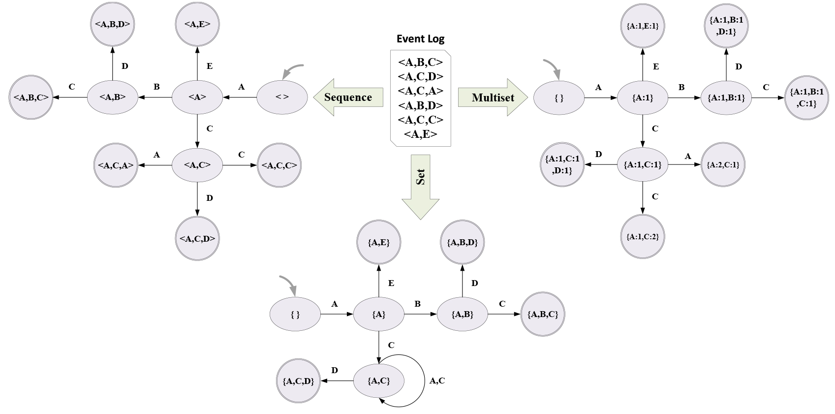

4. Remaining time prediction with auto-encoded transition system (AETS)

The overall framework of the proposed approach is depicted in Fig. 2. In the training stage, the given event log on one hand is used to mine a transition system, which abstracts the inherent global process information, on the other hand is used to generate the training data for constructing the remaining time prediction model. More specifically, a variety of features of historical traces recorded in the event log are extracted by taking into account both the global process information abstracted in the transition system and single instances’ own execution information. Then the raw sparse feature vectors are fed into a sparse auto-encoder to derive a more compact representation. Taking the historical traces with the compact representation as training data, a multi-layer perceptron (MLP) is trained for each state in the transition system for remaining time prediction. In the predicting stage, a given ongoing process instance is mapped to a state of the transition system, and the corresponding MLP model is applied to yield its remaining time. More details will be given in the following sections.

Figure 2.

The overall framework.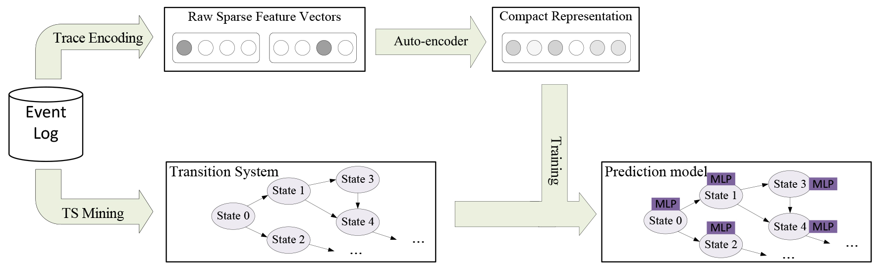

4.1 Transition system mining

Inspired by [17], we design the transition system mining algorithm, of which the details are given in Algorithm 4.1. The procedure of transition system mining involves two-round traversals of the input event log. In the first-round traversal (lines 2–8), the state of each trace prefix is calculated, based on which the state set $S$ of the transition system is constructed (lines 4–5). In the second-round traversal (lines 9–21), the states of each two adjacent prefixes $\sigma^{(k)}$ and $\sigma^{(k+1)}$ , and the representation of the $(k+1)$ -th event (i.e., $\sigma[k+1]$ ) between them are calculated (lines 11–13). Then the new prefix states and event representation are used to update the event representation set (line 15) and the transition set (line 18), respectively. After the two-round traversals finished, the state set $S$ , the event representation set $E$ , and the transition set $T$ of the transition system can be constructed.

[h] : TSMining[1] The event logs $L$ , the state representation function $\rho$ , the event representation function $\pi$ . Transition system $TS=(S,E,T)$ $S,E,T\leftarrow\varnothing$ ; $\sigma\in L$ $k\leftarrow 0$ to $|\sigma|$ $\rho(\sigma^{(k)})\notin S$ $S\leftarrow S\cup{\{\rho(\sigma^{(k)})\}}$ $\sigma\in L$ $k\leftarrow 0$ to $|\sigma|-1$ $s\leftarrow\rho(\sigma^{(k)})$ $e\leftarrow\pi(\sigma[k+1])$ $s^{\prime}\leftarrow\rho(\sigma^{(k+1)})$ $e\notin E$ $E\leftarrow E\cup{\{e\}}$ $(s,e,s^{\prime})\notin T$ $T\leftarrow T\cup{\{(s,e,s^{\prime})\}}$ $TS=(S,E,T)$

With the proposed process mining algorithm, a transition system is automatically discovered from the given event log, free of laborious efforts of domain experts. This would be desirable especially in case of large-volume event logs or lack of prior domain knowledge. We nevertheless note that our proposed remaining time prediction framework in Fig. 2 takes transition system as a module for trace encoding, thus offering the flexibility of incorporating transition systems either mined from event log or available as a prior.

4.2 Trace encoding

In order to take account into various factors affecting the remaining time of process instances, we propose to use a new form of trace encoding, including trace event features and trace state features, which encode the execution information of single trace, and related global process information, respectively.

4.2.1 Trace event encoding

Trace event encoding mainly considers the events and the associated attributes in a trace. Due to the heterogeneity of event attributes, we design different encoding schemes for three types of attributes, i.e., discrete attributes, continuous attributes, and datetime-type attributes.

Discrete attributes

We use one-hot encoding for discrete attributes, e.g., activity name, practitioner. Specifically, let a discrete attribute takes values from $P$ , an event with attribute value $p\in P$ is encoded as $\mathbf{v}=(0,\cdots,0,1,0,\cdots,0)\in\{0,1\}^{|P|}$ , with $|\mathbf{v}|=1$ .

Continuous attributes

We use discretization-based encoding for continuous attributes, e.g., execution time and cost. Specifically, let a continuous attribute takes values from $[\min,\max]$ , we divide the interval into $N$ equal bins. An event with attribute value $p$ is discretized by $p^{\prime}=\lfloor\frac{p-\min}{\max-\min}\cdot N\rfloor$ , then the feature vector is obtained by using one-hot encoding as done for discrete attributes.

Datetime-type attributes

Datetime is an indispensable field recorded in event logs because process instances are essentially time-sensitive event sequences. Thus we particularly design encoding scheme for datetime-type attributes. To be more specific, we treat every fields of a datetime value, i.e., year, month, week, day and hour, as discrete attributes, and concatenate the encodings of each fields. Taking a datetime-type value “2012/4/10 5:13” as an example, the field values “2012”, “4”, “10” and “5” are encoded as discrete values separately.

As the number of events in different traces is not always the same, we only consider the $m$ last events occurred in a trace when constructing the trace event encodings. Specifically, given a trace prefix $\sigma^{(k)}=<e_{1},\cdots,e_{k}>$ , the trace event encoding is constructed by:

$\displaystyle\mathbf{v}(\sigma^{(k)})=\mathbf{v}(e_{k-m+1})\oplus\cdots\oplus% \mathbf{v}(e_{k})$ (1)

where $\oplus$ denotes vector concatenation operation. $\mathbf{v}(e_{i})(k-m+1\leqslant i\leqslant k)$ is the encoding vector of event $e_{i}$ constructed by concatenating the encoding vector of each attribute of the event:

$\displaystyle\mathbf{v}(e_{i})=\mathbf{v}(e_{i}.a)\oplus\mathbf{v}(e_{i}.% \textit{start})\oplus\mathbf{v}(e_{i}.\textit{end})\oplus\mathbf{v}(e_{i}.p_{1% })\oplus\cdots\oplus\mathbf{v}(e_{i}.p_{(|P|)})$ (2)

where $\mathbf{v}(e_{i}.a)$ , $\mathbf{v}(e_{i}.\textit{start})$ , $\mathbf{v}(e_{i}.\textit{end})$ and $\mathbf{v}(e_{i}.p_{j})(1\leqslant j\leqslant|P|)$ are the encoding vectors for the running activity, start time, end time, and other attributes of $e_{i}$ , respectively.

Note that the vector of a trace prefix with length less than $m$ is zero-padded.

4.2.2 Trace state encoding

The states of transition system essentially represent running states of the overall business system. Each ongoing process instance (i.e., trace prefix) can be mapped to a state of transition system, which reflects the state of the business system at the time when the process instance is running. For each of the three forms of state representations, we design the corresponding state encoding scheme, respectively.

Formally, let the set of all events in an event log $L$ be $E$ , and the set of all event representations be $\Pi=\{\pi(e)|e\in E\}$ . For ease of the subsequent presentation, we write the event representation set as $\Pi=\{\pi_{1},\cdots,\pi_{|\Pi|}\}$ . The encoding scheme for the three forms of state representations are as follows:

(1)
SET: Given a set state $S=\{s_{1},\cdots,s_{|S|}\}$ , its encoding vector is $[v_{1},\cdots,v_{|\Pi|}]$ , where

$\displaystyle v_{i}=\left\{\begin{array}[]{ll}1,&\text{if}\ \pi_{i}\in S\\ 0,&\text{if}\ \pi_{i}\notin S\\ \end{array},\right.$ (3)
(2)
MULTISET: Given a multiset state $S=\{s_{1}:c(s_{1}),\cdots,s_{|S|}:c(s_{|S|})\}$ , its encoding vector is $[v_{1},\linebreak\cdots,v_{|\Pi|}]$ , where

$\displaystyle v_{i}=\left\{\begin{array}[]{ll}c(\pi_{i}),&\text{if}\ \pi_{i}% \in S\\ 0,&\text{if}\ \pi_{i}\notin S\\ \end{array},\right.$ (4)
(3)
SEQUENCE: Given a sequence state $S=\langle s_{1},\cdots,s_{n}\rangle$ , its encoding vector is constructed by concatenating the trace event encodings of its last $m$ states. For the state with length $n<m$ , its event encoding is zero-padded.

We give an example for the above encoding scheme for ease of understanding. Suppose the set of event representation is $\Pi=\{A,B,C,D,E,F\}$ , given a set state $s_{1}=\{A,B,C,D\}$ , a multiset state $s_{2}=\{A:1,B:2,C:1,D:1\}$ , and a sequence state $s_{3}=<A,B,B,C,D>$ . The corresponding state vectors are

$\displaystyle\mathbf{v}(s_{1})=[1,1,1,1,0,0]$ $\displaystyle\mathbf{v}(s_{2})=[1,2,1,1,0,0]$ (5) $\displaystyle\mathbf{v}(s_{3})=[0,0,0,1,0,0,0,0,1,0,0,0](m=2)$
4.3 Dimension reduction

After obtaining the event encoding vector and the state encoding vector, the trace vectors are formed by concatenating these two types of encoding vectors. Commonly, each events have a number of discrete attributes, and the one-hot encoding adopted above easily lead to high-dimensional and sparse feature vectors, which can hinder training effective machine learning models. To tackle the sparsity issue, we use sparse auto-encoder to reduce the dimension of raw trace encoding vectors and derive more compact feature vectors for traces.

Auto-encoder [20] is an unsupervised neural network model, which consists of an input layer, one or several hidden layers and an output layer. The task of auto-encoder is to reconstruct the input data from the low-dimensional representation generated by the hidden layers. Figure 3 illustrates the architecture of an auto-encoder, in which the part from the input layer and hidden layers is called as encoder, and that from hidden layers to the output layer called as decoder.

The input of auto-encoder is the trace encoding vector $\mathbf{x}=[x_{1},x_{2},\cdots,x_{n}]$ . First, the encoder obtains a hidden representation $\mathbf{h}$ of the trace encoding vector:

$\displaystyle\mathbf{h}=W_{2}(\textit{tanh}(W_{1}\mathbf{x}+\mathbf{b}_{1}))+% \mathbf{b}_{2}$ (6)

Then the decoder obtains the reconstruction of the trace encoding vector $\mathbf{x^{\prime}}$ according to the hidden representation:

$\displaystyle\mathbf{x^{\prime}}=\textit{sigmoid}(W_{4}\cdot\textit{tanh}(W_{3% }\cdot\mathbf{h}+\mathbf{b}_{3})+\mathbf{b}_{4})$ (7)

Here, $W_{1},W_{2},W_{3},W_{4}$ and $\mathbf{b}_{1},\mathbf{b}_{2},\mathbf{b}_{3},\mathbf{b}_{4}$ are learnable parameters that represent the transformation matrix and bias vector of each layer in the auto-encoder.

The aim of auto-encoder, i.e., reconstructing the trace encoding vectors, can be formalized as minimizing the following loss:

$\displaystyle\ell^{\text{(ae)}}(\mathbf{x})=|\mathbf{x}-\mathbf{x^{\prime}}|^{2}$ (8)

In this work, the stacked auto-encoder, as shown in Fig. 4, is used to derive the hidden features of input traces. The stacked auto-encoder is composed of several cascaded auto-encoders. The hidden feature vector extracted from the $i$ -th layer auto-encoder is fed into the $(i+1)$ -th layer auto-encoder for feature reconstruction. Finally, the condensed trace representation is obtained at the last layer auto-encoder.

Figure 3.

The architecture of auto-encoder.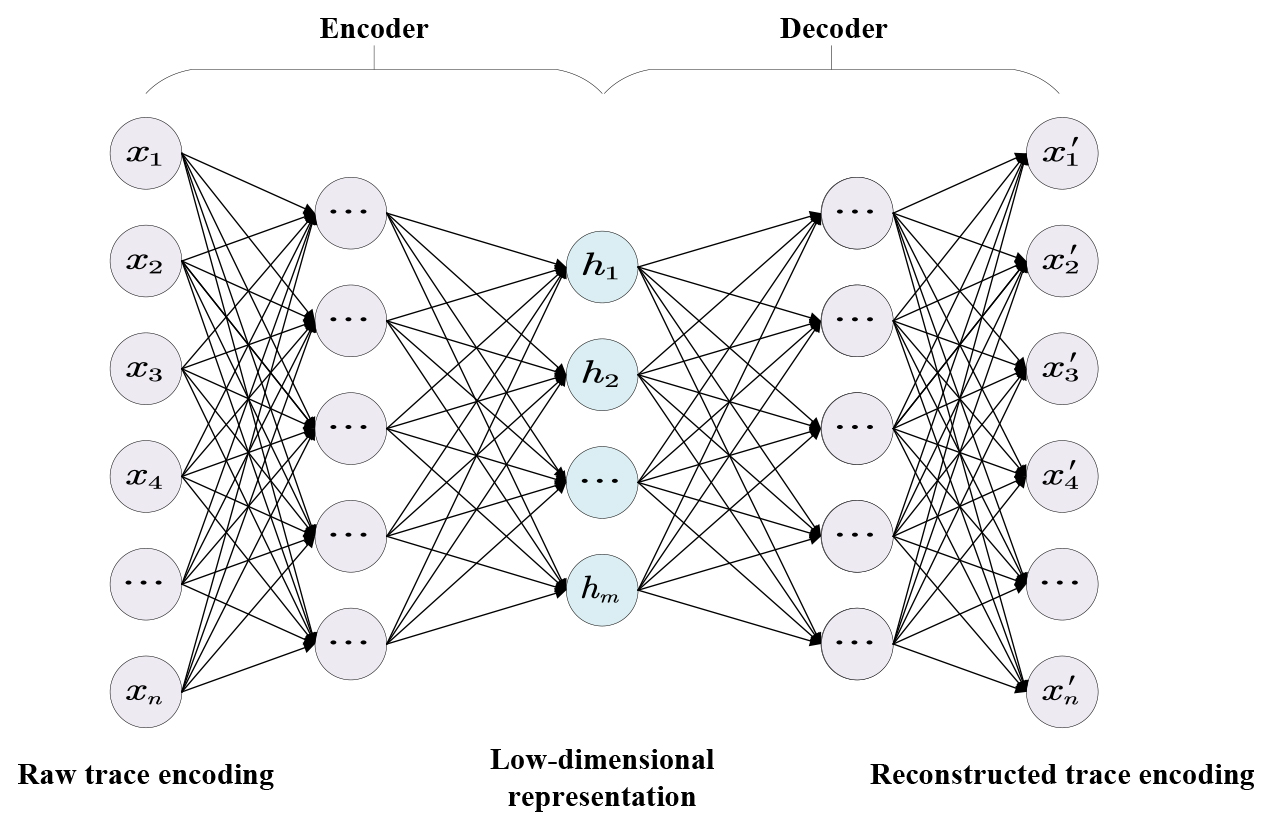

Figure 4.

The structure of stacked auto-encoders.

4.4 Model training

The remaining time prediction model is constructed by using the condensed representation of traces. In particular, we first generate a training set from a given query log, then train multi-layer perceptrons in a transfer learning manner as the remaining time prediction model.

4.4.1 Generating training set

Given an event log $L=\{\sigma_{1},\cdots,\sigma_{|L|}\}$ , we generate the set of trace prefixes as follows:

$\displaystyle L^{*}=\{\sigma^{(k)}\big{|}\forall\sigma\in L,1\leqslant k% \leqslant|\sigma|\}$ (9)

The trace prefix set is then divided by the states of the transition system $TS=(S,E,T)$ mined from the event log $L$ . Specifically, the trace prefix subset of a state $s\in S$ can be written as:

$\displaystyle L_{s}^{*}=\{\sigma^{(k)}\big{|}\forall\sigma^{(k)}\in L^{*},\rho% (\sigma^{(k)})=s\}$ (10)

Finally, the training set is generated by the condensed low-dimensional feature vector of each trace prefix in $L^{*}$ obtained through the stacked auto-encoders, and the remaining time of each trace prefix which is taken as the learning target:

$\displaystyle D_{s}=\{(\mathbf{h}(\sigma^{(k)}),\textit{remain}(\sigma^{(k)}))% \big{|}\forall\sigma^{(k)}\in L_{s}^{*}\}$ (11)

4.4.2 Training multi-layer perceptron

We train a three-layer perceptron (as shown in Fig. 5) for each state in the transition system as the remaining time prediction model. The input to each model is a trace feature vector $\mathbf{h}=[h_{1},h_{2},\cdots,h_{m}]$ . The output is the predicted remaining time $y$ , which is calculated as follows:

$\displaystyle\mathbf{z}^{(1)}=\textit{sigmoid}(U_{1}\mathbf{h}+\mathbf{b}_{1})$ $\displaystyle\mathbf{z}^{(2)}=\textit{sigmoid}(U_{2}\mathbf{z}^{(1)}+\mathbf{b% }_{2})$ (12) $\displaystyle y=U_{3}\mathbf{z}^{(2)}+\mathbf{b}_{3}$

where $\mathbf{z}^{(1)}$ and $\mathbf{z}^{(2)}$ are the outputs of the first and second layers, respectively. $U_{1},U_{2},U_{3}$ and $\mathbf{b}_{1},\mathbf{b}_{2},\mathbf{b}_{3}$ are learnable parameters that represent the transformation matrix and bias vector of each layer.

The following L1 loss is used for training the three-layer perceptron:

$\displaystyle\ell^{\text{(mlp)}}(\sigma^{(k)})=|y(\sigma^{(k)})-\textit{remain% }(\sigma^{(k)})|$ (13)

where $y(\sigma^{(k)})$ and $\textit{remain}(\sigma^{(k)})$ denote the predicted and true remaining time of trace prefix $\sigma^{(k)}$ , respectively.

Figure 5.

The architecture of three-layer perceptron.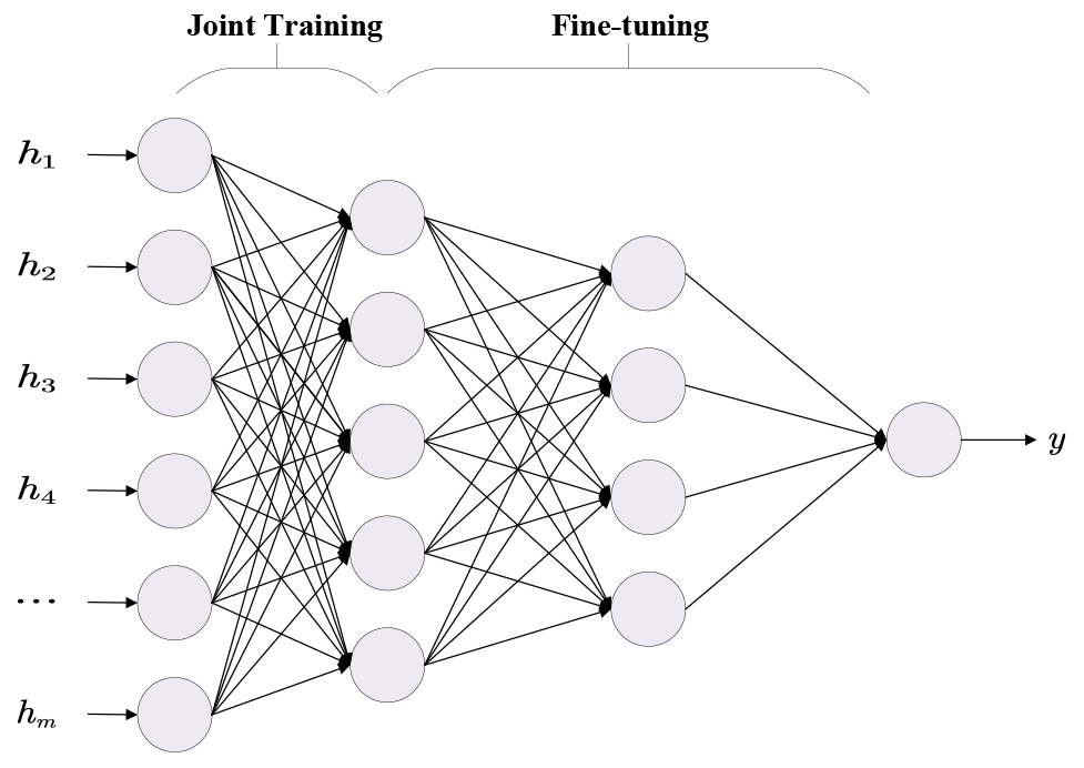

It should note that due to the potentially large amount of states in a transition system, the training set after divided by states tends to be much smaller; however, it is well recognized that limited training data easily leads to overfitting of neural networks. Inspired by recent developments in transfer learning [2], we propose to jointly train the multi-layer perceptrons for each states to tackle the overfitting problem. First, the multi-layer perceptrons for each states in the transition system are jointly trained using all the training set generated from the given event log. This stage can be viewed as pre-training for the remaining time prediction models. Then, for each state in the transition system, the parameters of the first layer in the three-layer perceptrons (i.e. $U_{1}$ and $\mathbf{b}_{1}$ ) are fixed, and the parameters of other layers (i.e. $U_{2}$ , $U_{3}$ and $\mathbf{b}_{2}$ , $\mathbf{b}_{3}$ ) are fine-tuned with the training set corresponding to each state.

Actually, states in a transition system are not necessarily independently with each other as longer states are formed by a series of transitions from shorter states, making the remaining time prediction models for each states also interrelated. The proposed joint training strategy is also advantageous in accounting for the correlation among the states in addition to tackling the overfitting problem.

Figure 6.

Statistics of datasets w.r.t. execution time.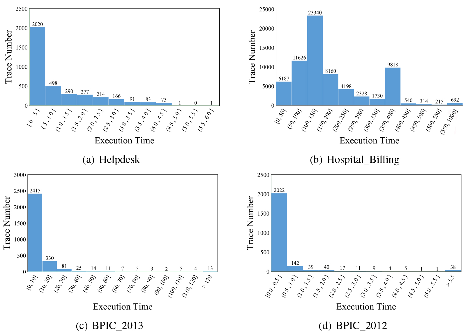

5. Experiments

5.1 Datasets

To evaluate the effectiveness of the proposed remaining time prediction approach, we use the following four real event logs from different domains:

(1)
Helpdesk: an event log recording the ticketing management process of the help desk of a software company;
(2)
Hospital_Billing: an event log from financial modules of the ERP system of a regional hospital;
(3)
BPIC_2013: an event log from an incident management system of an IT company;
(4)
BPIC_2012: an event log recording the application process for personal loan or overdraft within a global financing organization.

Basic statistics of the four datasets are shown in Table 2. Figure 6 illustrates the statistics of traces w.r.t. execution time for each of the four datasets. Before used for the experiments, these datasets are preprocessed by filtering out traces with concurrent events and noises. The traces with lengths less than 3 are also filtered out.

Table 2
Basic statistics of datasets

Dataset Trace number Event number Activity number Max trace length Min trace length

Helpdesk 3714 13328 9 14 3

Hospital_Billing 69148 410931 18 217 3

BPIC_2013 2915 14965 12 26 3

BPIC_2012 2329 12543 9 37 3

5.2 Experiment settings

Dataset	Trace number	Event number	Activity number	Max trace length	Min trace length
Helpdesk	3714	13328	9	14	3
Hospital_Billing	69148	410931	18	217	3
BPIC_2013	2915	14965	12	26	3
BPIC_2012	2329	12543	9	37	3

5.2.1 Baselines

The following three types of remaining time prediction approaches are used as baselines in the experiments:

(1)
TS (Transition System) [17] is the traditional process-model-based remaining time prediction approach. We specifically use three different state representations, i.e., set, multiset, and sequence, denoted as TS-set, TS-multiset, and TS-sequence, respectively.
(2)
DATS (Data-aware Transition System) [9] proposes an extension of traditional transition system – data-aware transition system – for remaining time prediction. The above three different state representations are used to constructed the data-aware transition system, denoted as DATS-set, DATS-multiset and DATS-sequence, respectively.
(3)
LSTM (Long Short-Term Memory) [14] is the traditional deep-learning-based remaining time prediction approach.

As for the proposed remaining time prediction approach, we also use the three different state representations, denoted as AETS-set, AETS-multiset and AETS-sequence, respectively. The main parameters of the proposed approach are tuned using a development set over the following ranges:1
¹
The codes are available at https://www.github.com/wj-ni/AETS/.

(1)
The dimension of condensed feature vectors of traces: $\{8,16,32,64\}$ ;
(2)
The number of neurons in the layers of multi-layer perceptron: $\{8,12,16,24,32\}$ ;
(3)
Learning rate: $\{10^{-2},10^{-3},10^{-4}\}$ ;
(4)
The number of training epoch: $\{80,90,100\}$ ;
(5)
Optimization algorithm: Adam.

5.2.2 Evaluation measures

We evaluate the performance of the proposed approaches and baselines using Mean Absolute Error (MAE) and Mean Squared Error (MSE), which have been widely used in regression tasks. Given an evaluation set $D=\{(\sigma^{(k)},\textit{remain}(\sigma^{(k)}))\}$ , MAE and MSE are calculated as follows:

$\displaystyle\textit{MAE}=\sum_{((\sigma^{(k)},\textit{remain}(\sigma^{(k)}))% \in D)}{|y(\sigma^{(k)})-\textit{remain}(\sigma^{(k)})|}$ $\displaystyle\textit{MSE}=\sum_{((\sigma^{(k)},\textit{remain}(\sigma^{(k)}))% \in D)}{(y(\sigma^{(k)})-\textit{remain}(\sigma^{(k)}))^{2}}$

where $y(\sigma^{(k)})$ and $\textit{remain}(\sigma^{(k)})$ denote the predicted and true remaining time for a trace prefix $\sigma^{(k)}$ in the evaluation set, respectively. In general, lower values of MAE and MSE indicate better-performed remaining time prediction models.

5.3 Overall results

The results of all the compared approaches are summarized in Table 3. In this experiment, we randomly split each dataset into three 70%-15%-15% parts, each taken as the training set, testing set and evaluation set, respectively. The partition is repeated 5 times and the average MAE/MSE values are reported. It can be seen that the proposed approach achieves the best performance in most cases, which directly verifies the effectiveness of the proposed auto-encoded transition system for the remaining time prediction task. By comparing the proposed approach with baselines, we can make the following further observations:

(1)
Compared to the traditional transition-system-based approaches (i.e., TS-set, TS-multiset and TS-sequence), the approaches fusing machine learning or deep learning techniques with transition system (i.e., DATS-set, DATS-multiset and DATS-sequence, as well as the proposed AETS-set, AETS-multiset and AETS-sequence) perform better in most cases (except in terms of MSE on BPIC_2012). This indicates the advantages of the combination of heterogeneous models over single ones in the remaining time prediction task.
(2)
Among the two types of approaches based on extended transition systems, the proposed AETS performs much better than DATS. Note that the main difference between them is that AETS uses deep learning (i.e., auto-encoder and multi-layer perceptron), whereas DATS uses traditional machine learning (i.e., support vector regression machine and decision tree). This result verifies the advantages of deep learning techniques in leveraging large-scale and noisy event logs for remaining time prediction. Furthermore, this advantage would be more significant in the case of even bigger event logs, as shown in Table 2 where the improvements of AETS are more significant on bigger event logs, e.g., Hospital_Billing and BPIC_2013.
(3)
Among the three types of state representations, the sequence representation (i.e., TS/DATS/AETS-sequence) performs slightly better than the multiset representation (i.e., TS/DATS/AETS-sequence), while both superior to the set representation (i.e., TS/DATS/AETS-set). This is mainly because the transition system constructed with sequence and multiset state representation tends to have more states, leading to finer-granular division of the event log and more targeted remaining time prediction models trained on each states.
(4)
The proposed AETS outperforms all the baselines with an exception on the BPIC_2012 dataset in terms of MSE. One reason is that the multi-layer perceptron for remaining time prediction is trained with L1 loss, which is essentially the same to the evaluation measure MAE, making AETS tends to perform better in terms of MAE than MSE. We also checked the BPIC_2012 dataset in more detail, and find that many traces did not end normally, which will be assigned with a large remaining time in the training set. This can be seen in Fig. 6d where the distribution of traces of the BPIC_2012 dataset exhibits a long yet heavy tail. The prediction errors on these traces tend to be large and have a greater impact on the evaluation results when measured by MSE.

Table 3
Remaining time prediction results of all compared approaches

Helpdesk Hospital_Billing BPIC_2013 BPIC_2012

MAE MSE MAE MSE MAE MSE MAE MSE

TS-set 7.800 98.438 72.622 11011 10.456 410.422 1.745 14.479

TS-multiset 7.401 92.643 72.401 10986 8.801 328.702 1.584 14.189

TS-sequence 7.313 91.283 72.404 10989 8.431 283.736 1.584 14.189

DATS-set 6.312 99.384 56.562 10424 6.427 354.488 1.503 17.328

DATS-multiset 6.305 101.874 56.192 10371 6.523 329.686 1.381 16.826

DATS-sequence 6.183 100.682 56.088 10338 6.099 270.289 1.381 16.826

LSTM 5.981 93.044 55.818 7389 5.139 231.175 1.415 16.664

AETS-set 5.707 82.627 39.330 7445 4.751 227.051 1.346 16.387

AETS-multiset 5.565 81.553 38.894 7376 4.485 159.593 1.312 16.043

AETS-sequence 5.423 76.154 39.323 7432 4.088 111.829 1.317 16.757

Figure 7.
Remaining time prediction results before and after removing abnormal traces.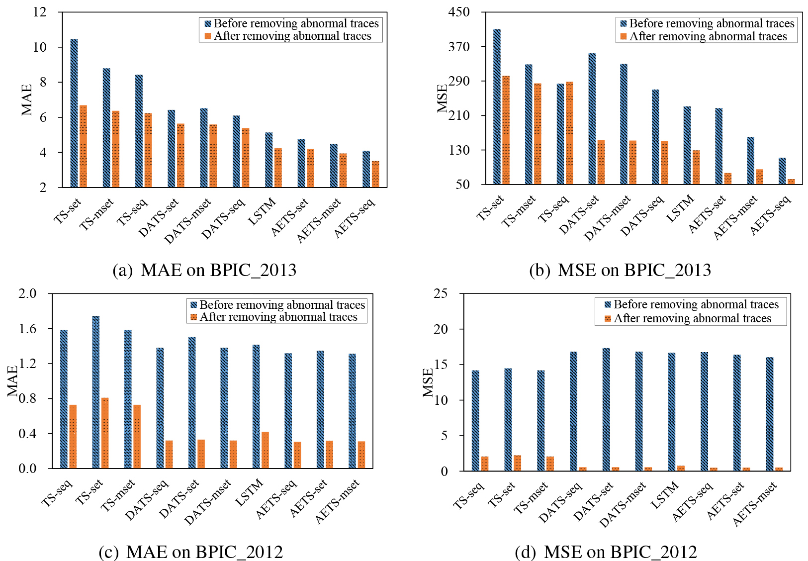

As a matter of fact, as shown Fig. 6, the four datasets used in the experiment exhibit two types of trace distributions w.r.t. execution time. That is, traces in the Helpdesk, BPIC_2013 and BPIC_2012 datasets roughly follow exponential distributions, whereas the distribution of traces in the Hospital_Billing dataset is more of a Gaussian mixture with three peaks at (100, 150], (350, 400] and (550, 1000], respectively. If we look in more detail, we see heavier tails in the BPIC_2013 and BPIC_2012 datasets, which imply a number of abnormal traces existing in the two datasets. To further evaluate the impact of abnormal traces on time prediction approaches, we remove the traces with very large execution time (i.e., larger than 120 and 5.5 in the BPIC_2013 and BPIC_2012 datasets, respectively) and compare the performance of each time prediction approaches which is shown in Fig. 7.

Figure 8.
Comparison of w/o auto-encoder.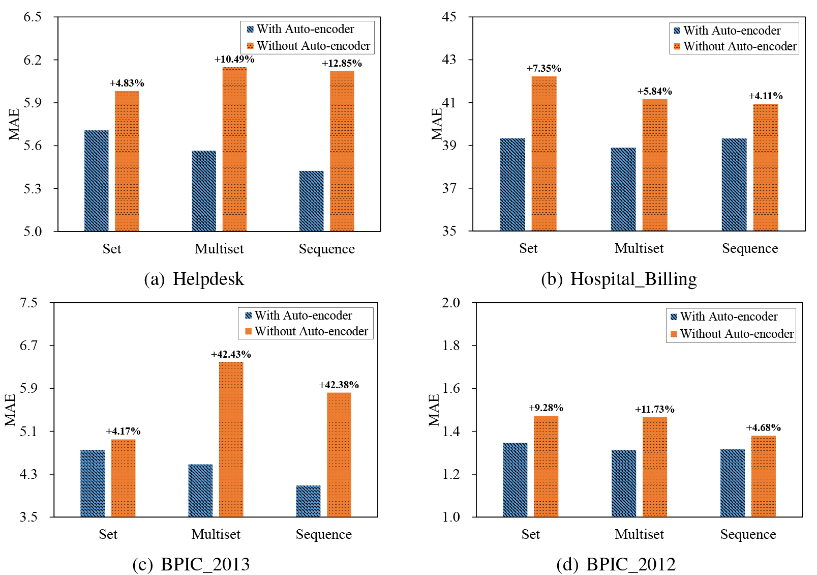

Figure 9.
Comparison of w/o transfer learning.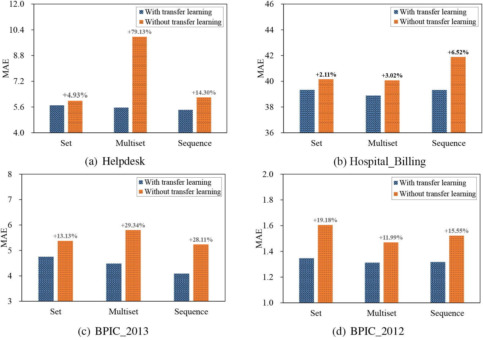

Figure 10.
Comparison of w/o transfer learning on different states.

Not surprisingly, it can be seen that after removing abnormal traces, the performance of every time prediction approach is significantly improved. The improvements are much more notable when evaluated with MSE. This is mainly attributed to the fact that the traces with large execution time actually dominate the MSE evaluation results. It also should be noted that the proposed AETS exhibits more significantly improved performance compared to baselines in terms of both evaluation measures on the datasets with abnormal traces removed, which verifies the superiority of our proposed time prediction approach. From this experiment, lessons we can learn is that it can be beneficial to remove abnormal traces (e.g., that with relatively large execution time) before applying remaining time prediction approaches.
5.4 Analysis

	Helpdesk	Hospital_Billing	BPIC_2013	BPIC_2012
	MAE	MSE	MAE	MSE	MAE	MSE	MAE	MSE
TS-set	7.800	98.438	72.622	11011	10.456	410.422	1.745	14.479
TS-multiset	7.401	92.643	72.401	10986	8.801	328.702	1.584	14.189
TS-sequence	7.313	91.283	72.404	10989	8.431	283.736	1.584	14.189
DATS-set	6.312	99.384	56.562	10424	6.427	354.488	1.503	17.328
DATS-multiset	6.305	101.874	56.192	10371	6.523	329.686	1.381	16.826
DATS-sequence	6.183	100.682	56.088	10338	6.099	270.289	1.381	16.826
LSTM	5.981	93.044	55.818	7389	5.139	231.175	1.415	16.664
AETS-set	5.707	82.627	39.330	7445	4.751	227.051	1.346	16.387
AETS-multiset	5.565	81.553	38.894	7376	4.485	159.593	1.312	16.043
AETS-sequence	5.423	76.154	39.323	7432	4.088	111.829	1.317	16.757

5.4.1 The impact of dimension reduction by auto-encoder

In this section, we analyze the impact of auto-encoder on dimension reduction experimentally. We specifically train remaining time prediction models with the following two strategies:

(1)
With Auto-encoder: The raw encoding vectors of traces are condensed by auto-encoder before used as the input of multi-layer perceptrons as described in Section 4.3.
(2)
Without Auto-encoder: The raw encoding vectors of traces are directly used as the input of multi-layer perceptrons.

Both the above remaining time prediction models use the same transition systems that are built with the sequence, set and multiset state representations, respectively.

The performance of the two remaining time prediction models in terms of MAE is shown in Fig. 8. It can be seen that the remaining time prediction models with auto-encoder consistently and significantly outperform the ones without auto-encoder, regardless of datasets and state representations. More specifically, the advantage of auto-encoder is more significant with multiset and sequence state representation, mainly due to the fact that the raw trace encoding vectors are sparser when states in transition systems are represented as multiset and sequence. This result demonstrates that dimensionality reduction of trace encoding is vital for the success of the proposed approach.
5.4.2 The impact of transfer learning

In this section, we experimentally analyze the impact of the remaining time prediction model training strategy based on transfer learning. We specifically train remaining time prediction models with the following two strategies:

(1)
With transfer learning: The remaining time prediction models for each states in transition system are trained jointly as described in Section 4.4.2.
(2)
Without transfer learning: The remaining time prediction models for each states in transition system are trained separately.

Figure 9 shows the results of the above two training strategies in terms of MAE. It can be seen that transfer learning is consistently superior to separate training. It is worth noting that up to a 70% improvement is achieved on the Helpdesk dataset. This verifies the importance of transfer learning for training high-quality remaining time prediction models.

In order to further explore the advantage of the proposed model training strategy, we conduct a more detailed analysis of the remaining time prediction results. Figure 10 shows the remaining time prediction results w.r.t. each state of the transition system, where the horizontal axis corresponds to each state and the vertical axis shows the corresponding MAE value. Here, the states are sorted according to the number of trace prefixes mapped to the state (i.e., $|L_{s}^{*}|$ in Eq. (10)). It can be seen that the transfer learning strategy outperforms separate training in most cases. Roughly speaking, the outperformance is more significant on the states with fewer trace prefixes. This provides evidence that the remaining time prediction models for the states with a small number of traces easily suffer from overfitting, and transfer learning can effectively make use of relevant data from other states to avoid the overfitting problem and improve the prediction accuracy.
6. Conclusion

In this paper, we have studied the task of predicting the remaining execution time of business process instances through fusing process modeling and deep learning techniques. Specifically, we have proposed an extension of transition system, i.e., Auto-Encoded Transition System (AETS) for remaining time prediction. Business process instances are first encoded by taking into account the execution information of each business process instance itself and the global state information of the information system. Then, stacked auto-encoder is used to tackle the high sparsity issue of raw trace encoding, and multi-layer perceptron is trained with a transfer learning strategy to construct the remaining time prediction models for each state of the transition system. Extensive experiments on four real event log datasets demonstrate that the proposed AETS can significantly reduce the MAE and MSE values of the remaining execution time prediction results compared with state-of-the-art baselines.

As future work, we plan to explore more advanced transfer learning strategy that can leverage the correlation among the states in transition system, such that the remaining time prediction models for different states can be jointly trained in a more effective manner. Furthermore, how to improve the interpretability of deep-learning-based remaining time prediction model is worth further exploration.

Footnotes

Acknowledgments

This work is partially supported by Natural Science Foundation of China (Grant No. 61602278, 71704096, and U1931207), the Taishan Scholars Program of Shandong Province (Grant No. TS20190936), and the Science and Technology Support Plan of Youth Innovation Team of Shandong Higher School (Grant No. 2019KJN024).

References

Augusto

Conforti

Dumas

La Rosa

Maggi

F.M.

Marrella

Mecella

and Soo

, Automated discovery of process models from event logs: Review and benchmark, IEEE Transactions on Knowledge and Data Engineering 31(4) (2018), 686–705.

Erhan

Courville

Bengio

and Vincent

, Why does unsupervised pre-training help deep learning? in: The 13th International Conference on Artificial Intelligence and Statistics, 2010, pp. 201–208.

Jimenez-Ramirez

Barba

Fernandez-Olivares

Del Valle

and Weber

, Time prediction on multi-perspective declarative business processes, Knowledge and Information Systems 57(3) (2018), 655–684.

Lee

W.L.J.

Parra

Munoz-Gama

and Sepulveda

, Predicting process behavior meets factorization machines, Expert Systems with Applications 112 (2018), 87–98.

Leontjeva

Conforti

Di Francescomarino

Dumas

and Maggi

F.M.

, Complex symbolic sequence encodings for predictive monitoring of business processes, in: International Conference on Business Process Management, Springer, 2016, pp. 297–313.

Navarin

Vincenzi

Polato

and Sperduti

, Lstm networks for data-aware remaining time prediction of business process instances, in: IEEE Symposium Series on Computational Intelligence, 2017, pp. 1–7.

Pasquadibisceglie

Appice

Castellano

and Malerba

, Using convolutional neural networks for predictive process analytics, in: International Conference on Process Mining, IEEE, 2019, pp. 129–136.

Polato

Sperduti

Burattin

and de Leoni

, Data-aware remaining time prediction of business process instances, in: International Joint Conference on Neural Networks, IEEE, 2014, pp. 816–823.

Polato

Sperduti

Burattin

and de Leoni

, Time and activity sequence prediction of business process instances, Computing 100(9) (2018), 1005–1031.

10.

Rogge-Solti

and Weske

, Prediction of business process durations using non-markovian stochastic petri nets, Information Systems 54 (2015), 1–14.

11.

Senderovich

Di Francescomarino

Ghidini

Jorbina

and Maggi

F.M.

, Intra and inter-case features in predictive process monitoring: A tale of two dimensions, in: International Conference on Business Process Management, Springer, 2017, pp. 306–323.

12.

Senderovich

Weidlich

Gal

and Mandelbaum

, Queue mining for delay prediction in multi-class service processes, Information Systems 53 (2015), 278–295.

13.

Tama

B.A.

and Comuzzi

, An empirical comparison of classification techniques for next event prediction using business process event logs, Expert Systems with Applications 129 (2019), 233–245.

14.

Tax

Verenich

La Rosa

and Dumas

, Predictive business process monitoring with lstm neural networks, in: International Conference on Advanced Information Systems Engineering, Springer, 2017, pp. 477–492.

15.

Teinemaa

Dumas

Maggi

F.M.

and Di Francescomarino

, Predictive business process monitoring with structured and unstructured data, in: International Conference on Business Process Management, Springer, 2016, pp. 401–417.

16.

Teinemaa

Dumas

Rosa

M.L.

and Maggi

F.M.

, Outcome-oriented predictive process monitoring: Review and benchmarkï¼Œ ACM Transactions on Knowledge Discovery from Data 13(2) (2019), 1–57.

17.

Van der Aalst

W.M.

Schonenberg

M.H.

and Song

, Time prediction based on process mining, Information Systems 36(2) (2011), 450–475.

18.

Verenich

Dumas

Rosa

M.L.

Maggi

F.M.

and Teinemaa

, Survey and cross-benchmark comparison of remaining time prediction methods in business process monitoring, ACM Transactions on Intelligent Systems and Technology 10(4) (2019), 1–34.

19.

Verenich

Nguyen

La Rosa

and Dumas

, White-box prediction of process performance indicators via flow analysis, in: Proceedings of the 2017 International Conference on Software and System Process, 2017, pp. 85–94.

20.

Wang

Yao

and Zhao

, Auto-encoder based dimensionality reduction, Neurocomputing 184 (2016), 232–242.

21.

Zhao

Chen

and Cao

, Method of time prediction for business process, Journal of Chinese Computer Systems 40(2) (2019), 42–48.

Predicting remaining execution time of business process instances via auto-encoded transition system

Abstract

Keywords

1. Introduction

3. Concepts

Table 1 An example event log

4.2 Trace encoding

4.2.1 Trace event encoding

4.4.1 Generating training set

5.1 Datasets

5.2.1 Baselines

5.3 Overall results

5.4.1 The impact of dimension reduction by auto-encoder

Footnotes

Acknowledgments

References

Table 1
An example event log