Anomaly repair-based approach to improve time series forecasting

Abstract

Time series forecasting has many practical applications in a variety of domains such as commerce, finance, medicine, weather, environment, and transportation. There exist so many methods developed for time series forecasting. However, most of the forecasting methods do not pay attention to anomalies in time series even though time series are sensitive to anomalies. Anomaly patterns cause negative effects on the accuracy of time series forecasting. In this paper, we propose a novel anomaly repair-based approach to improve time series forecasting in the case of anomaly existence. In our approach, an effective time series forecasting framework, EPL_S_X, is proposed with anomaly smoothing as a pre-processing stage and any existing time series prediction algorithm X. In particular, our proposed approach consists of three steps including detecting anomalies, repairing anomalies by using our smoothing method, and forecasting time series using preprocessed time series. Experimental results on several time series datasets reveal that our proposed approach improves remarkably the accuracy of many existing time series forecasting methods. It also outperforms the two robust time series forecasting methods that are based on exponential and Holt-Winters smoothing. With such better prediction performance, our approach is not only more effective but also more useful when dealing with anomalies in time series forecasting.

Keywords

Time series forecasting anomaly detection anomaly smoothing k-nearest neighbors Holt-Winters artificial neural network

1. Introduction

In time series data mining, forecasting in time series is one of the most complex and challenging problems, as mentioned in the review by De Gooijer and Hyndman [6]. Indeed, time series prediction has attracted many researchers as shown in their proposed works [1, 2, 4, 9, 16, 17, 18, 19, 21, 24, 28, 33]. This is understandable due to the popularity of time series in a variety of application domains and the significance of the forecasting task in practice.

From the existing research works, time series forecasting methods can be categorized into two groups. The first group includes classical methods such as ARIMA model, regression, and exponential smoothing, while the second one consists of machine-learning based methods such as k-nearest-neighbors (k-NN), artificial neural networks (ANNs), and support vector machines (SVMs). Lago et al. [16] concluded that machine learning-based methods brought out higher prediction accuracy than statistical ones.

Some recent forecasting research works based on machine learning are listed as follows. In [21], Notton et al. proposed ANNs for solar radiation estimation and forecasting in energy applications. The work in [4] used ARIMA-ANN hybrid method and empirical mode decomposition to improve forecasting accuracy of time series. Lu et al. [18] proposed a hybrid model based on improved fruit fly optimization algorithm and support vector machines for short-term load forecasting of urban gas. Bao et al. [1] proposed a hybrid model using sequential ANN and Holt-Winters models for time series prediction. Besides, Bouktif et al. [2] proposed single and multi-sequence deep learning models for short and medium term electric load forecasting. Lago et al. [16] proposed deep learning approaches and empirical comparison with traditional algorithms to forecast spot electricity prices. In short, the features of these forecasting methods in common are: (1) they only applied forecasting for some specific time series data types and (2) they do not take into account anomalies explicitly.

In practice, one of the most recurrent problems in forecasting is the presence of anomalies (outliers, noises, anomalous patterns, discords). In addition, most of the forecasting methods are sensitive to anomalies. For example in [8], Gelper et al. mentioned that anomalies can affect the Holt-Winters exponential smoothing method in two ways. First, the predicted values are affected since they depend on the current and past values of the time series including the anomalies. The second impact of anomalies involves the selection of the parameters used in the updating technique. These influences might lead to incorrect forecasted results and decreasing the effectiveness of the forecasting methods.

To alleviate the negative effects of anomalies in time series forecasting, there have been some research works which apply anomaly detection and repair to improve data before forecasting [30, 5, 25]. However most of these works use statistical-based methods in anomaly detection which are workable in specific applications. Statistical-based methods fit the statistical model or distribution to the dataset and apply a statistical inference test to determine an observation is an anomaly or not. But the main drawback of statistical methods is that data often do not match a particular distribution.

Realizing that time series anomaly detection has many beneficial uses for data mining, including data cleaning and forecasting, in this work, we aim to devise a novel anomaly repair-based approach to improve time series forecasting in the presence of anomalies. This approach consists of three main steps: anomaly detection, anomaly repair, and prediction. These steps help handling anomalies in a general context where time series data of various kinds can be applied and any prediction method can be utilized after the time series is cleaned out of the anomalies. To realize this purpose of the work, we propose a time series forecasting framework, named EPL_S_ $X$ , where $X$ is any aforementioned existing prediction method such as linear regression, $k$ -nearest neighbors, artificial neural networks, or support vector machines. Moreover, EPL_S_ $X$ is equipped with the most recent anomaly detection method, EP-Leader-DTW, for anomaly detection in time series with both high accuracy and efficiency [27]. In addition, we devise an anomaly smoothing method to adjust anomaly patterns into normal ones so that the repaired time series can be processed with higher performance by the selected $X$ prediction method.

Compared to the existing methods for time series forecasting in the case of anomaly existence, our method is the first general framework that performs anomaly detection and repair in order to improve forecasting accuracy without requiring that the data fit any statistical model or distribution. In fact, our proposed approach is a data-driven method which does not require any domain knowledge from experts. Besides, an extensive empirical evaluation has been done on several datasets with different trend, and seasonal characteristics and from various application domains. The experimental results show that our method outperforms the existing time series forecasting methods and especially improves remarkably the prediction performance of many existing time series prediction methods. In short, our method is not only effective but also practical when reducing the influence of anomalies in time series forecasting.

The rest of the paper is organized as follows. Section 2 presents some related works on time series forecasting and anomaly detection. Section 3 describes the proposed anomaly-repair-based approach for time series forecasting. Section 4 reports the main experiments to check the effectiveness of our approach. Finally, Section 5 gives some conclusions and future works.

2. Related works

2.1 Time series forecasting

In time series mining, time series forecasting is a task that takes a time series $T=t_{1},t_{2},\ldots,t_{m}$ with the length m and then predicts the values at each next time point, e.g. $t_{m+1},t_{m+2},\ldots$ The effectiveness of the task is reflected via the accuracy of its predicted values. In terms of a learning process, this task can be resolved with supervised learning.

In practice, time series forecasting is a popular but non-trivial task because of the popularity and characteristics of time series in a variety of application domains. Indeed, time series are present in many applications where objects and their relationships are recorded over time. In addition, time series in each application may have their own characteristics. Some typical ones are trend, seasonality, periodicity, irregularity, randomness, etc. These characteristics challenge the time series forecasting task. The task is more challenging when noises, outliers, or anomalies exist in the input time series.

In the existing works, trend and seasonal time series have been considered in forecasting task with different proposed methods. As introduced in [32], a trend in a time series is the long-term change in the level of the data. In the case of time stretching, the series moves upward, it is said that the data show a positive trend. Otherwise, the series moves downward, it is said that the data show a negative trend. Trends in time series clearly violate the condition of stationary. A seasonal pattern occurs in a time series when there is a regular variation in the level of the data that repeats itself at the same time each year. The term “season” is used to represent a period of time before the behavior begins to repeat itself. A cyclical (periodic) pattern is represented by a wavelike upward and downward movement of the data around the long-term trend. Cyclical fluctuations are of longer durations and are less regular than seasonal fluctuations.

Among the existing forecasting methods, a few of them [8, 17] paid attention to handling anomalies. In the work [8], Gelper et al. proposed two Robust Forecasting versions for exponential smoothing, a well-known classical method for time series forecasting. Exponential smoothing is a simple technique used to forecast a time series without the necessity of fitting a parametric model. It is based on a recursive computing scheme, where the forecastings are updated for each new incoming observation. The Holt-Winters method, also called as double exponential smoothing, is an extension of exponential smoothing for trended and seasonal time series. In [8], two proposed versions for Holt-Winters method, called RHW and RHW’, can handle outliers in time series. These two robust versions perform outlier detection and smoothing before prediction. However, they can detect and smooth out only point anomalies while time series in real world areas usually contain subsequence anomalies. Gelper et al. perform outlier detection and smoothing by applying Kalman filter [20] to the state-space model associated with exponential and Holt-Winters smoothing. Experimental results on two datasets reveal that RHW and RHW’ bring out better prediction results than the original Holt-Winters method.

Loc and Anh [17] proposed a method of anomaly detection and repair to improve Holt-Winters forecasting. This method can detect and smooth out subsequence anomalies. However, one drawback in this method is that it detects anomalies by using BFDD (brute-force discord discovery) algorithm proposed by Keogh et al. [12] which is a simple and inefficient window-based method for anomaly detection in time series. Therefore, this method can be improved upon.

In short, both of the above-mentioned forecasting methods used simple methods in anomaly preprocessing for only exponential smoothing forecasting method. By contrast, we propose a forecasting approach that can handle anomaly detection and repair with a combination of more efficient techniques and can work for any forecasting method.

2.2 Anomalies in time series

A top anomaly pattern in a time series is a subsequence that is maximally different from other subsequences in that time series. This is the most commonly-used and intuitive definition for anomaly subsequence, given by Keogh et al. [12]. Notice that anomaly in this definition is subsequence anomaly, not point anomaly. That means the anomalies we consider in this paper are contextual and based on a local context [5]. Figure 1 illustrates a top anomaly in an electrocardiogram (ECG) time series [27].

Figure 1.

An anomaly in ECG time series.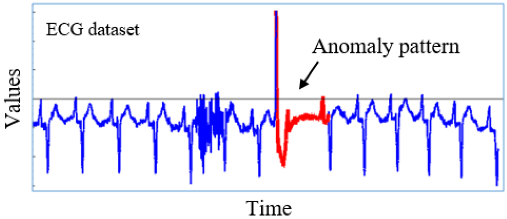

The anomalies might reduce the performance of a time series forecasting task because they introduce abnormal behaviours that are not common ones observed with the time series. They may mislead the process to incorrect forecast results. Therefore, anomalies in the input time series of the task should be detected and repaired to ensure the effectiveness of the forecasting results.

Outlier/noise/anomaly handling is a well-studied topic in knowledge discovery. However, surprisingly, this topic is still limited in time series forecasting as previously reviewed with only two research works [8, 17]. This situation motivates us to develop an approach to deal with time series forecasting with the presence of anomalies.

To handle this problem, we first need to detect where anomalies are located in time series. Up to now a lot of anomaly detection methods have been proposed for time series data. They are listed as Brute-Force and HOT SAX of Keogh et al. in 2005 [12], WAT of Bu et al. in 2007 [3], a method based on segmentation and Finite State Automata by Salvador and Chan in 2005 [23], a method based on segmentation and cluster-based outlier detection by Kha and Anh in 2015 [15] and EP-Leader-DTW proposed by Thuy et al. [27]. Among these anomaly detection methods, EP-Leader-DTW, in our previous work, is the most recent one that can detect anomalies accurately and efficiently with Dynamic Time Warping, the most effective distance measure for time series data. Therefore, in our proposed approach for time series forecasting, EP-Leader-DTW is used to detect anomalies in time series before forecasting. With high accuracy of anomaly detection, EP-Leader-DTW does not bring out false alarms in time series anomaly detection.

2.3 EP-Leader-DTW algorithm

EP-Leader-DTW is the anomaly detection algorithm proposed by Thuy et al. [27] with four steps:

•
Step 1: Segmentation. This step uses the important extreme points method proposed by Fink and Gandhi [7] to segment time series into subsequences.
•
Step 2: Transformation. A homothetic transformation is performed to transform subsequences of different lengths into subsequences of the same length by using the average length of all the extracted subsequences.
•
Step 3: Clustering. The Leader algorithm proposed by Hartigan [10] is used to cluster similar subsequences into the same clusters. EP-Leader-DTW then calculates the anomaly scores of all the subsequences by using the formulas given by Thuy et al. [27].
•
Step 4: Anomaly Detection. EP-Leader-DTW finally determines the subsequence with the largest anomaly score as the top anomaly subsequence of the time series.

As compared to the other anomaly detection methods, EP-Leader-DTW does not require users to predetermine the length of the anomaly subsequence. Instead, EP-Leader-DTW uses two parameters, compression rate – R and clustering threshold – $\varepsilon$ , which are easily examined for appropriate values. With the use of DTW distance, EP-Leader-DTW has better anomaly detection accuracy than the other previous anomaly detection methods which use Euclidean distance [27]. For more details about EP-Leader-DTW algorithm, interested readers can refer to the paper in Thuy et al. [27].

The following is a brief comparison between Euclidean and DTW distance measures to clarify the effectiveness of EP-Leader-DTW when DTW is used.

Euclidean distance (ED) is the most commonly-used distance measure between two time series. ED measures the dissimilarity between two time series by aligning the point-to-point observations at the same time. Therefore, ED is very sensitive to distortions in the time axis. However, the advantage of ED is its linear execution time.

Figure 2.
Euclidean distance (left) and DTW distance (right) [13].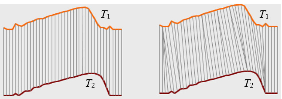

By contrast, DTW is suitable for calculating a distance between two time series that do not need to be aligned point-to-point at the same time (see Fig. 2) [22]. In addition, DTW can compute the distance between two time series with different lengths. Moreover, as mentioned in the work of Wang et al. [29], DTW is significantly more accurate than ED for time series classification on small datasets while converged to ED on larger datasets. Nevertheless, the disadvantage of DTW is high time complexity. In order to use DTW efficiently, methods based on DTW need to use some techniques to speed-up DTW calculation. A well-known speed-up technique is lower-bounding. One of the popular lower-bounding techniques is LB_Keogh proposed by Keogh and Ratanamahatana in 2005 [13].
3. EPL_S_X: The proposed time series forecasting approach

To handle the time series forecasting task in presence of anomaly patterns, we devise an anomaly repair-based framework, called EPL_S_ $X$ , where $X$ can be any existing time series prediction method. The details of our proposed approach are presented as follows.

3.1 Anomaly repair-based approach to time series forecasting

Anomaly handling is normally handled in the data preprocessing phase of a knowledge discovery process. Similarly, we define an anomaly repair stage as a data preprocessing phase before time series forecasting by any existing time series prediction method. Our approach consists of the three following main steps.

•
Step 1: Anomaly detection. In this step, the input time series is processed for finding anomalies if any. These anomalies are explicitly identified as abnormal subsequences in the input time series.
•
Step 2: Anomaly repair. The resulting anomalies in Step 1 are processed to become normal subsequences in the input time series. In other words, those anomalies are smoothed out of the time series. The input time series after this step is considered clean with no anomaly patterns.
•
Step 3: Prediction. The clean time series produced from Step 2 is then used for forecasting. Any time series forecasting method can be applied on this clean time series. Its output, which includes forecast data points, is also the output of our time series forecasting approach.

In our forecasting approach, no restriction on the data characteristics of time series is counted on. This implies that our approach is not bound with any specific kind of time series data or their application domains. Besides, in Step 2, our proposed approach tries only to clean anomalies and preserves all other information in the time series data.
3.2 Details of EPL_S_X

EPL_S_ $X$ is our time series forecasting approach, proposed along with the anomaly repair-based method as its preprocessing step. In this approach, EP-Leader-DTW [27] is chosen for anomaly detection in Step 1. Although there are many anomaly detection methods on time series, EP-Leader-DTW is the most recent one that can detect anomalies in time series with high effectiveness and efficiency. Anomaly repair process in Step 2 is then conducted with a combination of mean and max replacements. For time series prediction in Step 3, X is any existing time series prediction method such as linear regression, k-nearest neighbors, support vector machine, or artificial neural network.

The pseudo code of EPL_S_ $X$ is shown below.

Method: EPL_S_X

Input: Time series $T_{\textit{in}}$ , an existing time series prediction method $X$

Output: Predicted time series $T_{\textit{out}}$

Process:

1. Anomaly detection with EP-Leader-DTW

A $\leftarrow$ EP-Leader-DTW ( $T_{\textit{in}}$ )

2. Anomaly adjustment with Anomaly-Repair

$T^{\prime}\leftarrow$ Anomaly-Repair ( $T_{\textit{in}}$ , $A$ )

3. Prediction with an existing time series prediction method $X$

$T_{\textit{out}}\leftarrow X(T^{\prime})$

4. Return $T_{\textit{out}}$

The pseudo code of our smoothing method, Anomaly-Repair(), is presented as follows.

Method: Anomaly-Repair

Input: Time series $T_{\textit{in}}$ , set of anomaly patterns $A$

Output: Preprocessed time series $T^{\prime}$

Process:

1. Group formation.

Unusual_Group, Normal_Group $\leftarrow$ Split ( $T_{\textit{in}}$ , $A$ )

2. Unusual subsequence adjustment.

for each unusual subsequence $h\_s$ in Unusual_Groupdo

if ( $h\_s$ is a homothetic transformed subsequence in $T_{\textit{in}}$ ) then

real_s $\leftarrow$ Extract ( $T_{\textit{in}}$ , $h\_s$ )

Unusual_Group $\leftarrow$ Unusual_Group $\cup$ {real_s}

end if

end for

for each unusual subsequence $s$ in Unusual_Groupdo

for each data point $p$ in $s$ do

$\textit{p.value}\leftarrow\textit{Average}$ ( $T_{\textit{in}}$ , p.position, s.length)

if ( $\textit{p.value}>\textit{Maximum}$ (Normal_Group)) then

$\textit{p.value}\leftarrow\textit{Maximum}$ (Normal_Group)

end if

end for

$T^{\prime}\leftarrow\textit{Merge}$ (Unusual_Group, Normal_Group)

3. Return $T^{\prime}$

After detecting the positions of anomaly subsequences, a smoothing technique is defined to clean these anomaly subsequences. There have been some smoothing techniques to clean outliers or noises out of a time series, such as, moving average, exponential smoothing and regression methods. However, due to the specific properties of our EP-Leader-DTW algorithm, in this work, we devise a new technique to perform anomaly smoothing. This technique is performed by our Anomaly-Repair module. The target of this module is to decrease unusually great values or increase unusually small values of data points toward the values which are considered normal. The question is how to determine which values are unusually large and which values are unusually small and then how to adjust their values so that no anomaly exists under any form in the preprocessed time series for prediction. The details of Anomaly-Repair method are described as follows.

Based on anomaly scores computed by EP-Leader-DTW, we divide subsequences into two groups by using Split() function. The first group, Unusual_Group, contains the subsequences whose anomaly scores are approximately similar to that of the most unusual subsequence. The second group, Normal_Group, contains the rest of subsequences extracted from the time series. In this function, at first, the most anomaly subsequence is put into the Unusual_Group group. After that, all the subsequences whose anomaly scores are almost the same as that of the most anomaly subsequence are put into this unusual group. We can measure their score differences by means of an approximated score ratio, e.g. 10%. The remaining subsequences of the time series are put into the normal group.

Once these two groups are formed, anomaly repair is carried out to reduce the abnormal level of the anomalies in the unusual group. In this step, we examine each homothetic transformed subsequence which is anomaly and refer back to its corresponding real subsequences so that all the unusual subsequences of the input time series can be adjusted accordingly. To extract the real subsequence of a homothetic transformed subsequence $h\_s$ in the unusual group, Extract() function is used. Its returned real subsequence real_s is then inserted into the unusual group.

After the unusual group is updated, each of its members is considered for adjustment in a point-by-point manner. For each data point $p$ in an unusual subsequence s in the unusual group, let us denote s.length to be the length of the subsequence $s$ , p.value and p.position to be the value and the time position of this data point $p$ in its subsequence $s$ . The adjustment is made for the value of each data point p by replacing p.value with the average value of p.length data points right before the subsequence $s$ . We use Average() function to compute this average value for replacement. If the values of data points in anomaly subsequences after such smoothing are still greater than the largest normal value, they are set to the largest normal value. The largest normal value is the maximum value among data points of normal subsequences in the Normal_Group group. We use Maximum() function to return the largest normal value. This extra replacement step along with the average smoothing is valuable to avoid having extremely large values in the smoothed subsequences.

Finally, all the smoothed subsequences in the Unusual_Group group and those in the Normal_Group group are merged by means of Merge() function to produce the preprocessed time series $T^{\prime}$ which is now ready for the prediction process given by any selected time series prediction method X.

3.3 Characteristics of EPL_S_X

According to the design of EPL_S_ $X$ above, EPL_S_ $X$ is a time series forecasting framework rather than a specific approach in which $X$ can be chosen particularly for an application of time series forecasting. As discussed in Subsection 3.2, EPL_S_ $X$ does not exploit any data characteristics of the time series under consideration in its process or require that the data fit some statistical model or distribution. Such a property implies that a wide range of time series data can be supported by EPL_S_ $X$ in forecasting. Moreover, if there is no anomaly present in the input time series, the prediction performance of EPL_S_ $X$ will be reduced to that of $X$ . Such a reduction indicates a positive improvement of EPL_S_ $X$ over $X$ where $X$ is any existing time series prediction method. Nevertheless, since anomalies are usually present in time series of various application domains, EPL_S_ $X$ will be more suitatble for time series forecasting in practice.

The main characteristics of EPL_S_ $X$ in comparison with the two methods proposed by Gelper et al. [8] can be summarized as follows:

•
EPL_S_ $X$ is a general framework that can be applied on any existing time series prediction method $X$ . By contrast, the Robust Smoothing methods in [8] are fixed with only exponential and Holt Winters smoothing.
•
EPL_S_ $X$ performs explicit anomaly detection and then smoothing out anomalies, while the Robust Smoothing methods implicitly embed the Kalman filter in the forecasting model. In Robust Exponential methods, outlier smoothing is applied even though there is no anomaly in the time series.
•
EPL_S_ $X$ is investigated with an intensive empirical evaluation on 14 datasets of varying lengths and with different trend, and seasonal characteristics in various application domains for checking the generality of the proposed method. In a less general context, the two proposed methods in [8] were evaluated on only two datasets for a comparison with only one baseline method.

4. Experimental evaluation

In this section, we evaluate the proposed forecasting approach EPL_S_ $X$ with the two following research questions and their corresponding experiment settings.

4.1 Research questions

•
Question 1: Does our proposed approach EPL_S_ $X$ outperform the Robust Smoothing methods in [8] for time series forecasting?
•
Question 2: Can our anomaly-repair strategy improve some typical prediction methods in terms of prediction accuracy?

Notice that, Gelper et al. [8] proposed Robust Holt-Winters method (RHW) and a variant of RHW (RHW’) for forecasting time series in presence of outliers. These two methods were evaluated on the Thermostat Sales time series (with trend) and the Resex time series (with trend and seasonality). Different from RHW and RHW’, our approach is more general. Therefore, we will use a version of our proposed approach which uses a particular forecasting method to compare with the two Robust Smoothing methods.

As for the second question, the generality of EPL_S_ $X$ is tested to confirm that our approach can improve the performance of several well-known prediction methods on several datasets of various application domains. For comparison, we will experiment two cases without and with the anomaly-repair strategy (i.e. EPL_S_ $X$ and $X$ ), for each time series prediction method X.
4.2 Experiment settings

For empirical evaluation, we implemented the comparative forecasting methods in Visual C#. All the experiments were conducted on an HP Intel ${}^{\@setsize{\scriptsize}{9.5pt}{\viiipt}{\@viiipt}\textregistered}$ Core ${}^{\text{TM}}$ i7-3630 QM CPU with 2.40 GHz processor, 8 GB RAM.

In our experiments, 14 datasets are used as described in Table 1. The first four time series datasets are downloaded from the webpage [26]. The next five time series datasets are from the webpage [11]. The tenth and eleventh datasets are downloaded from the UCR Time series Classification/Clustering [14]. The last three datasets are downloaded from the UCI webpage [31]. Shown in Table 1, these datasets come from various application domains such as transportation, environment, commerce, medicine, finance, economy, production, and energy. Their lengths are also varying. In addition, most of them have trends together with seasonal variations although the patterns are quite different from dataset to dataset. Besides these datasets, we also used the Thermostat Sales time series in [8] for the experimented related to Question 1.

To ensure the presence of anomalies in tested time series, anomaly embedding was made at random positions in all the 14 above-mentioned datasets as well as Thermostat Sales dataset. Each dataset was divided into two parts. The first part includes 2/3 data points of time series and the second one includes the rest data points. The first part is used for training and the second one for testing. Finally, only one-step-ahead forecasting was considered in all of the experiments.

Table 1
Datasets used in the experiments

No.	Description	Dataset name	Application domain	Data characteristics	Length
1	Monthly airline passenger numbers at Pan Am Airline	Pan Am	Transportation	Seasonal, trend	144
2	Monthly atmospheric CO2 in Mauna Loa, Hawaii	CO2	Environment	Seasonal, trend	468
3	Monthly sales of a gift store in Queensland, Australia	Fancy	Commerce	Seasonal, trend	84
4	Average monthly deaths from lung diseases in England	Mdeaths	Medicine	Seasonal	72
5	Monthly milk production in Australia	Milk	Production	Seasonal, trend	119
6	Monthly sales of a company in Chatfield, Australia	Sales	Commerce	Seasonal, trend	77
7	Quarterly beer production in Australia	Beer	Production	Seasonal, trend	154
8	Quarterly consumer expenditure in Australia	Expenditure	Finance	Seasonal, trend	144
9	Average quarterly consumer budget plan in USA	Quarterly	Finance	Seasonal, trend	52
10	Power demand	Power	Energy	Periodic	6000
11	Stock data	Stock	Economy	Periodic	1000
12	BitCoin	BitCoin	Finance	Periodic	365
13	Oil	Oil	Energy	Periodic	281
14	S&P	S&P	Economy	Periodic	118

Regarding to the comparative prediction methods for the experiment related to Question 2, we used some well-known prediction methods such as linear regression (abbreviated as LR), k-nearest neighbors (k-NN), artificial neural networks (ANN), and the hybrid method proposed in [1] (Hybrid). Their parameter settings were made in the trial-and-error scheme. These prediction methods have been used for time series forecasting in the context of no concern about anomalies. In this experiment these methods are improved with our anomaly-repair strategy to become EPL_S_LR, EPL_S_kNN, EPL_S_ANN, and EPL_S_Hybrid, respectively. Among these comparative methods, for the experiment related to Question 1, we use EPL_S_kNN to compare with the two Robust Holt-Winters methods (RHW and RHW’) in [8].

For measuring the accuracy of the forecast results, we used the mean squared error (MSE), the mean absolute error (MAE), and the mean absolute percentage error (MAPE (%)) as follows.

$\displaystyle\textit{MSE}=\frac{1}{n}\sum_{t=1}^{n}(\widehat{y_{t}}-y_{t})^{2}$ (1) $\displaystyle\textit{MAE}=\frac{1}{n}\sum_{t=1}^{n}|{\widehat{y_{t}}-y_{t}}|$ (2) $\displaystyle\textit{MAPE}=\frac{100}{n}\sum_{t=1}^{n}\left|\frac{\widehat{y_{% t}}-y_{t}}{y_{t}}\right|$ (3)

In these equations, n is the length of time series, $y_{t}$ is the value in time series at time point t, and $\widehat{y_{t}}$ is the forecast value at time point $t$ . In the literature, MSE, MAE, and MAPE are commonly-used measures to evaluate the prediction performance of forecasting methods. All three criteria are all negative orientation scores, i.e. their lower values imply better forecasting methods.

4.3 Experimental results and discussions

In this subsection, we present the experimental results in Table 2 for the experiment related to Question 1 and those in Tables 3–8 for the experiment related to Question 2. In these tables, the best results are presented in bold.

Table 2
MSE values of RHW, RHW’ (Gelper et al. [8]), and EPL_S_ $k$ NN on Thermostat sales time series

	Gelper et al.’s proposed methods		EPL_S_ $k$ NN
	RHW’	RHW	Case a: outlier position $=$ 35	Case b: oulier position $=$ 7
Clean data	518	517	172	197

Table 3

MSE values for time series forecasting with LR, EPL_S_LR, k-NN, EPL_S_kNN without and with anomaly repair strategy

Dataset	LR	EPL_S_LR	k-NN	EPL_S_kNN
Pan Am	1930	1613	8412	5576
CO2	219	1	279	224
Fancy	143376499	28310337	90707424	70949879
Mdeaths	115409	101101	94452	48769
Milk	55906	3577	11970	11164
Sales	20504	16215	25913	24056
Beer	5892	25	11535	3765
Expenditure	5018410	1254612	26009528	7627081
Quarterly	17	1	48	17
Power	166	148	4416	3713
Stock	54	0	178	63
BitCoin	101357	86657	565590	560515
Oil	224	214	15	2
S&P	597545	3334	197276	165468

Table 4

MSE values for time series forecasting with ANN, EPL_S_ANN, Hybrid, EPL_S_Hybrid without and with anomaly repair strategy

Dataset	ANN	EPL_S_ANN	Hybrid	EPL_S_Hybrid
Pan Am	54422	886	24479	7259
CO2	957	82	8423	1717
Fancy	176384131	20246963	406064115	284511072
Mdeaths	1755733	243307	22374	12309
Milk	34542	3723	48398	1495
Sales	42688	15934	60412	42783
Beer	73414	187	60800	9347
Expenditure	31171013	3430043	108017426	64155790
Quarterly	18	1	45	21
Power	560	249	4152	3744
Stock	504	0	111	18
BitCoin	23831824	357183	1315110	1174823
Oil	438	260	31	21
S&P	2709156	113773	7761	6342

4.3.1 Question 1: Does our proposed method EPL_S_X outperform the Robust Smoothing methods in [8] for time series forecasting?

In this experiment, we compare the prediction performance of EPL_S_ $k$ NN method to those of the robust forecasting methods proposed by Gelper et al. [8]. The reason for this choice is that EPL_S_ $k$ NN is not the best method among the four prediction methods which apply our proposed anomaly-repair strategy. If the worst method of EPL_S_ $X$ is better than the two methods given by Gelper et al. [8], then other methods of EPL_S_ $X$ are too.

To be unbiased, we used the experimental results reported in Gelper et al. [8] to compare to those of our EPL_S_ $k$ NN method on the same dataset: Thermostat Sales time series.

In Fig. 3, we used the Thermostat Sales time series in two cases. Since there is no outlier in Thermostat Sales dataset, we embedded outliers (noises, anomalies) into this dataset at different positions. For the first case (3a), we create an outlier at position 35 and in the second case (3b), another outlier at position 7. We used these two different outlier positions to test the degree of influence of the outlier position on the outcome of the forecasting method. On Thermostat Sales time series, we also examined both EPL_S_ $k$ NN and $k$ -NN methods to check the effectiveness of EPL_S_ $k$ NN compared to $k$ -NN.

Figure 3.

Thermostat Sales time series forecasted by EPL_S_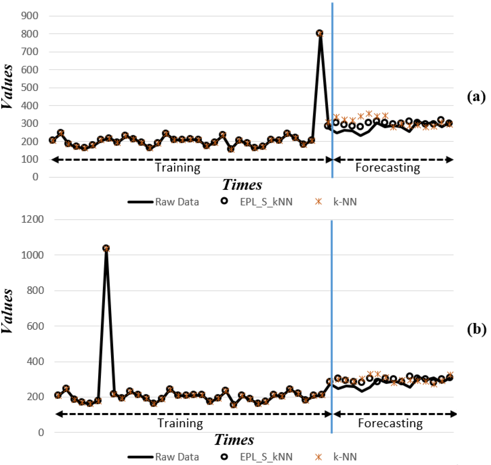 $k$ NN (circle) and by $k$ -NN (star), and the raw data (solid line) at two different outlier points (Case a: outlier position $=$ 35, Case b: outlier position $=$ 7).

For the experiments, we prepared training and test datasets for forecasting Thermostat Sales time series. Displayed in Fig. 3, the left part of the blue line shows a part of data used for training, the right part of the blue line shows the data forecasted by the two methods EPL_S_ $k$ NN and $k$ -NN compared to the real data of Thermostat Sales dataset. In both Fig. 3a and b, forecasted data points by EPL_S_ $k$ NN are closer to actual data points than forecasted data points by $k$ -NN. This reflects the effectiveness of smoothing outliers before forecasting in our EPL_S_ $k$ NN method.

Table 5

MAE values for time series forecasting with LR, EPL_S_LR, k-NN, EPL_S_kNN without and with anomaly repair strategy

Dataset	LR	EPL_S_LR	k-NN	EPL_S_kNN
Pan Am	34	24	75	62
CO2	13	1	14	13
Fancy	7579	3508	5894	5001
Mdeaths	298	254	269	182
Milk	190	32	73	54
Sales	121	112	120	113
Beer	60	4	86	46
Expenditure	1609	1009	4242	2315
Quarterly	3	1	5	3
Power	10	9	57	52
Stock	6	0	12	7
BitCoin	235	214	624	606
Oil	8	7	3	1
S&P	721	46	405	363

Table 6

MAE values for time series forecasting with ANN, EPL_S_ANN, Hybrid, EPL_S_Hybrid without and with anomaly repair strategy

Dataset	ANN	EPL_S_ANN	Hybrid	EPL_S_Hybrid
Pan Am	187	19	155	60
CO2	26	7	92	37
Fancy	10616	3114	14150	10800
Mdeaths	1139	384	117	99
Milk	136	41	150	31
Sales	178	95	197	150
Beer	248	12	242	83
Expenditure	4375	1576	9681	7004
Quarterly	3	1	5	4
Power	17	12	54	50
Stock	19	1	5	4
BitCoin	3952	478	983	933
Oil	18	11	5	4
S&P 1442	299	71	55

Shown in Table 2, we compared the MSE values obtained from [8] to those from our experiments using EPL_S_ $k$ NN on average. In this table, clean data mean the time series after smoothing anomalies. In the experiment of Gelper et al., outliers were embedded near the data point to be predicted. In our experiment, we added noises at the two different positions to check if our outlier-repair strategy works well or not when the outlier data points are located in different places. Notice that in case (3a) the outlier data point was so near to the data point to be predicted as shown in [8]. In case (3b) the outlier data point was far from the data point to be predicted.

From the results in Table 2, the MSE values of RHW and RHW’ methods are larger than those of EPL_S_ $k$ NN in both the cases. It is clear that no matter where the noise data point is, smoothing the noises by our proposed approach helps improve the forecasting results. In short, EPL_S_ $k$ NN is more effective than both RHW’ and RHW methods [8] in time series forecasting with the presence of anomalies.

4.3.2 Question 2: Can our anomaly-repair strategy improve some typical prediction methods in terms of prediction accuracy?

In Tables 3–8, we report the experimental results for three evaluation criteria collected from various comparative prediction methods over different datasets. In Tables 9 and 10, the improvement rates of EPL_S_ $X$ over X are reported where in all of the cases, X denotes a comparative prediction method such as LR, k-NN, ANN, or a hybrid one in [1], Hybrid. The improvement rate is calculated as the ratio of the prediction measure of X to that of EPL_S_ $X$ in terms of MSE, MAE, and MAPE. For Question 2, the experiment results aim to answer the question whether the typical prediction methods can increase their prediction accuracy when applying our anomaly-repair-based approach.

Table 7
MAPE values for time series forecasting with LR, EPL_S_LR, k-NN, EPL_S_kNN without and with anomaly repair strategy

Dataset	LR	EPL_S_LR	k-NN	EPL_S_kNN
Pan Am	11.0	7.0	19.6	16.3
CO2	3.9	0.3	4.1	3.7
Fancy	53.3	27.3	24.5	17.6
Mdeaths	31.8	23.6	21.4	14.6
Milk	20.6	3.8	8.6	6.3
Sales	51.5	46.5	23.6	21.4
Beer	11.7	1.3	17.2	9.0
Expenditure	4.3	2.8	8.2	4.6
Quarterly	12.0	4.3	20.2	13.0
Power	6.4	5.4	43.7	40.1
Stock	23.1	1.0	46.8	27.8
BitCoin	2.7	2.4	5.8	5.6
Oil	23.4	21.5	7.7	2.8
S&P	24.1	1.6	13.2	11.8

Table 8

MAPE values for time series forecasting with ANN, EPL_S_ANN, Hybrid, EPL_S_Hybrid without and with anomaly repair strategy

Dataset	ANN	EPL_S_ANN	Hybrid	EPL_S_Hybrid
Pan Am	58.8	5.9	46.2	15.5
CO2	7.6	2.3	26.3	10.7
Fancy	90.2	26.0	67.3	61.1
Mdeaths	158.2	42.8	9.7	8.2
Milk	13.4	5.4	14.7	3.7
Sales	88.0	35.7	50.1	35.3
Beer	50.7	3.8	50.5	18.9
Expenditure	11.0	4.4	18.9	13.6
Quarterly	11.7	3.8	1690.0	1342.0
Power	9.2	7.1	39.7	37.3
Stock	71.0	2.1	15.9	14.2
BitCoin	44.0	5.3	9.3	8.8
Oil	54.0	35.4	11.5	9.0
S&P	47.9	9.9	2.1	1.6

As for the simple forecasting method LR (linear regression), the MSE values from EPL_S_LR are smaller than those obtained from the pure LR for all of the 14 datasets. The MSE improvement rate of EPL_S_LR over LR is about 87.9 times on average. Similarly, MAE and MAPE values from EPL_S_LR are also smaller than those from the pure LR for all 14 datasets. In addition, the MAE improvement rate of EPL_S_LR over LR is about 6.3 times and the MAPE improvement rate is about 5.7 times on average. In sum, the prediction performance of LR using our anomaly repair strategy is remarkably better than that of LR without using our anomaly-repair strategy.

Not only LR but also all the other well-known forecasting methods like k-NN and ANN provide better prediction results when applying our anomaly-repair strategy over all the 14 datasets. For example, the MSE values obtained from EPL_S_kNN are smaller than those from the pure k-NN for all the 14 datasets. This is also reflected through the fact that the MSE improvement rate of EPL_S_kNN over k-NN is about 2.2 times. Similarly, for all the datasets, the MAE and MAPE errors produced by EPL_S_kNN are smaller than those by the pure k-NN. On average, the MAE improvement rate of EPL_S_kNN over k-NN is about 1.4 times and the MAPE improvement rate is about 1.5 times.

As for artificial neural network (ANN), EPL_S_ANN improves ANN in terms of prediction accuracy remarkably over all of the 14 datasets. The MSE, MAE, and MAPE improvement rates of EPL_S_ANN over ANN shown in Table 6 are about 142.5, 7.3, and 6.7 times, respectively. For example, for the very short time series dataset S&P, EPL_S_ANN can provide MSE value 23.81 times better than the one yielded by the pure ANN without anomaly detection and repair.

Table 9

Improvement rates of EPL_S_X over X where X is LR, k-NN

	\|	EPL_S_LR/LR		\|	EPL_S_k-NN/k-NN
Dataset	MSE	MAE	MAPE	MSE	MAE	MAPE
Pan Am	1.20	1.45	1.57	1.51	1.21	1.20
CO2	204.18	13.30	12.55	1.25	1.10	1.10
Fancy	5.06	2.16	1.96	1.28	1.18	1.39
Mdeaths	1.14	1.17	1.35	1.94	1.48	1.47
Milk	15.63	6.03	5.37	1.07	1.35	1.36
Sales	1.26	1.08	1.11	1.08	1.06	1.10
Beer	235.42	14.82	9.17	3.06	1.88	1.91
Expenditure	4.00	1.59	1.51	3.41	1.83	1.80
Quarterly	12.06	3.93	2.82	2.72	1.53	1.55
Power	1.12	1.14	1.17	1.19	1.10	1.09
Stock	568.63	23.21	23.14	2.82	1.68	1.68
BitCoin	1.17	1.10	1.10	1.01	1.03	1.04
Oil	1.05	1.08	1.08	7.90	2.73	2.74
S&P	179.25	15.57	15.34	1.19	1.12	1.12
Average	87.9	6.3	5.7	2.2	1.4	1.5

Table 10

Improvement rates of EPL_S_X over X where X is ANN, or Hybrid

Dataset	MSE	MAE	MAPE	MSE	MAE	MAPE
	\|	EPL_S_ANN/ANN		\|	EPL_S_Hybrid/Hybrid
Pan Am	61.41	9.94	9.98	3.37	2.57	2.98
CO2	11.64	3.52	3.32	4.91	2.48	2.47
Fancy	8.71	3.41	3.47	1.43	1.31	1.10
Mdeaths	7.22	2.97	3.70	1.82	1.19	1.17
Milk	9.28	3.28	2.51	32.37	4.88	3.95
Sales	2.68	1.87	2.46	1.41	1.31	1.42
Beer	392.43	20.80	13.44	6.51	2.91	2.67
Expenditure	9.09	2.78	2.50	1.68	1.38	1.39
Quarterly	15.49	4.56	3.10	2.18	1.24	1.26
Power	2.24	1.37	1.30	1.11	1.06	1.06
Stock	1382.92	33.59	33.52	6.14	1.36	1.12
BitCoin	66.72	8.26	8.25	1.12	1.05	1.06
Oil	1.68	1.67	1.53	1.48	1.28	1.27
S&P	23.81	4.82	4.82	1.22	1.29	1.29
Average	142.5	7.3	6.7	4.8	1.8	1.7

In addition to the single prediction methods as discussed above, our anomaly repair-based approach can improve a hybrid prediction method proposed in [1], denoted as Hybrid. This Hybrid method combines Holt-Winters’ exponential smoothing and artificial neural networks in order that it can take advantage of the benefits of the two methods. This is because the ANN model can capture nonlinear features hidden in the time series and the Holt-Winters’ exponential smoothing can capture some trend and seasonal features in the time series. The experimental results show that EPL_S_Hybrid can dramatically reduce MSE, MAE and MAPE errors over all the 14 datasets. The MSE, MAE, and MAPE improvement rates of EPL_S_Hybrid over the pure Hybrid are about 4.8, 1.8, and 1.7 times, respectively.

Figure 4.

Original time series (solid line), the predicted time series by EPL_S_kNN (circle line), and by the pure k-NN ( star line) on Expenditure dataset.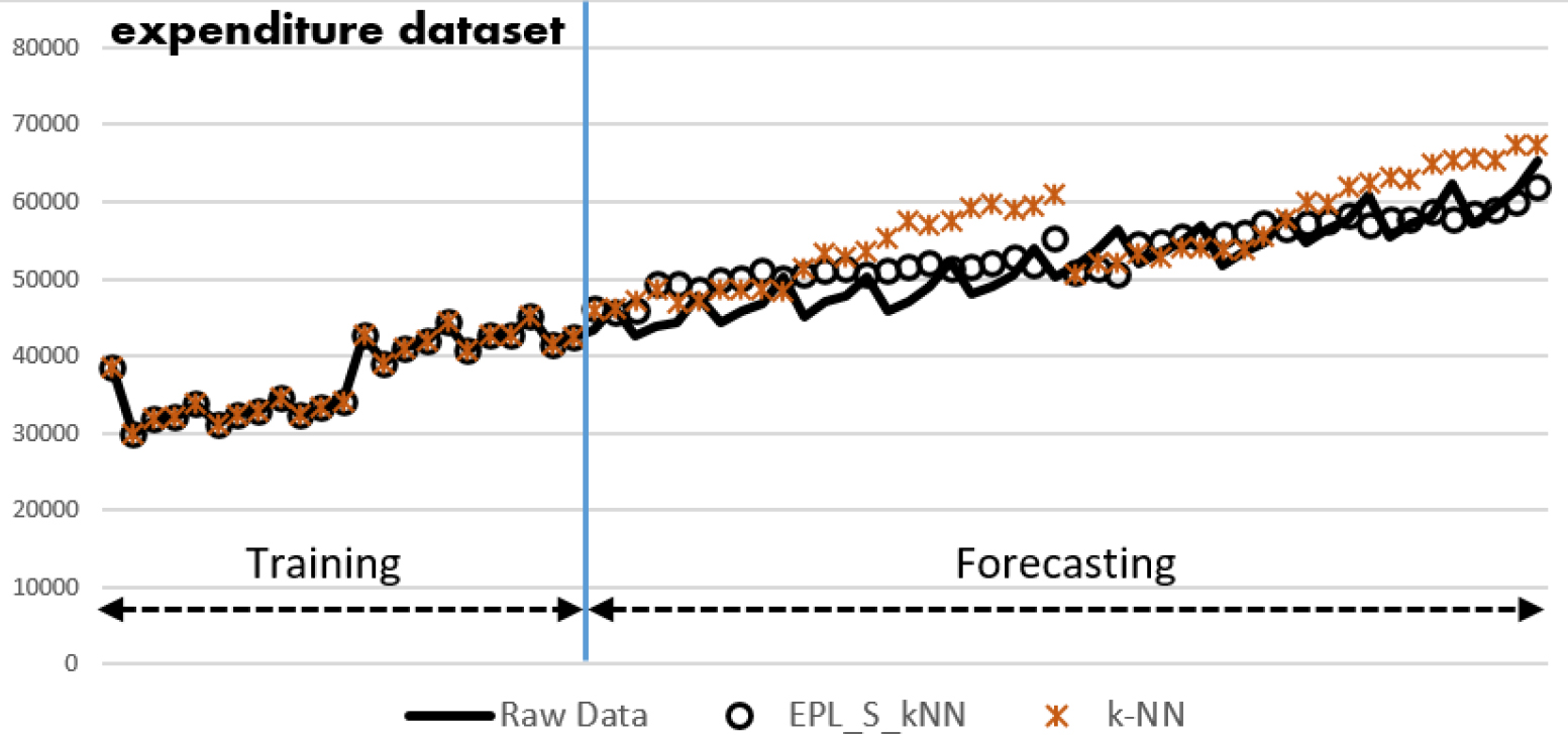

Figure 4 displays point-to-point comparison between actual values (in solid) and predicted values (by EPL_S_kNN in circle, or by k-NN in star) on Expenditure dataset. In Fig. 4, by using EPL_S_kNN, predicted data points are closer to actual data points than predicted data points by using k-NN. Due to space limitation, just only the experiment results on Expenditure dataset is illustrated graphically in Fig. 4. For the Expenditure dataset, we forecast 49 data points at the end of the training part of the time series.

Generally speaking, experimental results in Tables 3–10, and Fig. 4 indicate that the forecasting framework EPL_S_X brings out remarkably better forecast results than any comparative prediction method, X where X is LR, k-NN, ANN, or Hybrid on all the 14 datasets with different lengths and different periodic, trend, and/or seasonal characteristics from various application domains. From this experiment, it is recommended that in the presence of anomalies, an anomaly-repair based approach should be used before applying an existing prediction method in order to improve the prediction performance.

Our explanation to why the preprocessing with anomaly repair can improve forecasting accuracy is that the anomaly patterns in a time series may account for the dominance of its total variance. Models that ignore these anomaly patterns will result in a high variance thus poor forecasting accuracy.

5. Conclusions

Improving prediction accuracy is a very important problem in time series forecasting. So far, most of the time series forecasting methods do not take anomalies into account before forecasting although anomalies always appear in time series. Anomalies usually have a strong impact on the accuracy of the forecasting results. Handling them through a process of anomaly detection and repair before forecasting is thus necessary for several prediction applications.

In this paper, we propose a novel time series forecasting framework, EPL_S_ $X$ , which is an enhanced version of any existing prediction method X for better prediction performance in the case of anomaly existence. In particular, EPL_S_ $X$ tackles anomalies explicitly in two pre-processing phases: anomaly detection and anomaly smoothing before the selected method X is performed for predicting the time series. For anomaly detection, EP-Leader-DTW algorithm is used due to its high accuracy and efficiency. For anomaly smoothing, a combination of mean and max replacements is used for the unusual subsequence group obtained from anomaly detection of EP-Leader-DTW. These techniques result in our new anomaly-repair-based approach with the framework EPL_S_ $X$ .

Many experiments have been conducted on 14 datasets in many different application domains to confirm the effectiveness of our EPL_S_ $X$ method in time series forecasting. From the experiment results, we can draw two following conclusions. First, smoothing out anomalies helps increase the accuracy of time series forecasting remarkably for many typical prediction methods such as linear regression, k-nearest neighbors, support vector machines, artificial neural networks, and a hybrid method of Holt-Winters’ exponential smoothing and artificial neural networks [1]. Second, the EPL_S_kNN forecasting method performs better than Robust Holt-Winters methods [8], the two improved variants of Holt-Winters method, where outlier detection and repair are applied on time series before forecasting.

In the future, we intend to extend our method for online time series forecasting in many application domains that need on-line forecasting. Moreover, we will consider a new version of our framework by utilizing a deep neural network-based forecasting method.

Footnotes

Acknowledgments

This research is funded by Ho Chi Minh City University of Technology (HCMUT), VNU-HCM, under grant number BK-SDH-2022-8141217.

References

Bao

D.N.

N.D.

and Anh

D.T.

, A hybrid method for forecasting trend and seasonal time series, Proceedings of The 2013 RIVF International Conference on Computing & Communication Technologies-Research, Innovation, and Vision for Future (RIVF) (10 November 2013), pp. 203–208s.

Bouktif

Fiaz

Ouni

and Serhani

M.A.

, Single and multi-sequence deep learning models for short and medium term electric load forecasting, Energies 12(1) (2019), 149.

Leung

T.W.

A.W.C.

Keogh

Pei

and Meshkin

, WAT: Finding top-k discords in time series database, Proceedings of the 2007 SIAM International Conference on Data Mining, 2007, pp. 449–454.

Büyükşahin

Ü.Ç.

and Ertekin

Ş.

, Improving forecasting accuracy of time series data using a new ARIMA-ANN hybrid method and empirical mode decomposition, Neurocomputing 361 (2019), 151–63.

Chandola

Banerjee

and Kumar

, Anomaly detection: a survey, ACM Computing Surveys (CSUR), 41(3) (2009), 1–58.

De Gooijer

J.G.

and Hyndman

R.J.

, 25 years of time series forecasting, International Journal of Forecasting 22(3) (2006), 443–473.

Fink

and Gandhi

S.H.

, Important extrema of time series, Proceedings of IEEE International Conference on System, Man and Cybernetics, Montreal, Canada, 2007, pp. 366–372.

Gelper

Fried

and Croux

, Robust forecasting with exponential and Holt-Winters smoothing, Journal of Forecasting 29(3) (2010), 285–300.

Giao

B.C.

and Anh

D.T.

, An Application of Similarity Search in Streaming Time Series under DTW: Online Forecasting, Proceedings of 8th International Symposium on Information and Communication Technology-SoICT 2017, Nha Trang, Vietnam, 2017, pp. 10–17.

10.

Hartigan

JA.

, Clustering Algorithms, John Wiley & Sons, New York, 1975.

11.

Hyndman

R.J.

, Time Series Data Library, http://data.is/TSDLdemo. Accessed in 2014.

12.

Keogh

Lin

and Fu

, HOT SAX: Efficiently finding the most unusual time series subsequence, Proceedings of The fifth IEEE International Conference on Data mining (ICDM), 2005, pp. 226–233.

13.

Keogh

and Ratanamahatana

C.A.

, Exact indexing of dynamic time warping, Knowledge and information systems 7(3) (2005), 358–386.

14.

Keogh

Wei

and Ratanamahatana

C.A.

, The UCR Time series Classification/Clustering. Homepage: www.cs.ucr.edu/ẽamonn/time_series_data. Accessed in 2017.

15.

Kha

N.H.

and Anh

D.T.

, From Cluster-Based Outlier Detection to Time Series Discord Discovery, In Trends and Applications in Knowledge Discovery and Data Mining. PAKDD 2015 Workshops: Big PMA, VLSP, QIMIE, BAEBH, Ho Chi Minh City, Vietnam, May 19-21 X.L. Li et al. (Eds.), LNAI 9441, Springer, 2015, pp. 16–28.

16.

Lago

De Ridder

and De Schutter

, Forecasting spot electricity prices: Deep learning approaches and empirical comparison of traditional algorithms, Applied Energy 221 (2018), 386–405.

17.

Loc

T.D.

and Anh

D.T.

, Using Anomaly Detection to Improve Holt-Winters Method in Time Series Prediction, Proceedings of 3rd Asian Conference on Information Systems (ACIS 2014), Nha Trang, Vietnam December 1–3, 2014, pp. 143–150.

18.

Azimi

and Iseley

, Short-term load forecasting of urban gas using a hybrid model based on improved fruit fly optimization algorithm and support vector machine, Energy Reports 5 (2019), 666–77.

19.

Martínez

Frías

M.P.

Pérez

M.D.

et al., A methodology for applying k-nearest neighbor to time series forecasting, Artificial Intelligence Review 52(3) (2019).

20.

Martin

R.D.

and Thomson

D.J.

, Robust-resistant spectrum estimation, Proceedings of the IEEE 70, 1982, pp. 1097–1115.

21.

Notton

Voyant

Fouilloy

Duchaud

J.L.

and Nivet

M.L.

, Some applications of ANN to solar radiation estimation and forecasting for energy applications, Applied Sciences 9(1) (2019), 209.

22.

Ratanamahatana

C.A.

and Keogh

, Everything you know about Dynamic Time Warping is wrong, Proceedings of 3rd Workshop on Mining Temporal and Sequential Data, 2004, pp. 22–25.

23.

Salvador

and Chan

, Learning states and rules for time series anomaly detection, Applied Intelligence 23(3) (2005), 241–255.

24.

Son

N.T.

N.H.

and Anh

D.T.

, Time series prediction using pattern matching, Proceedings of 2013 International Conference on Computing, Management and Telecommunications (ComManTel), IEEE, 2013, pp. 401–406.

25.

Takeuchi

and Yamanishi

, A Unifying Framework for Detecting Outliers and Change Points from Time Series, IEEE transactions on Knowledge and Data Engineering 18(4) (2006), 482–492.

26.

The R project for Statistical Computing at http://www.r-project.org/. Accessed in 2014.

27.

Thuy

H.T.T.

Anh

D.T.

and Chau

V.T.N.

, Efficient segmentation-based methods in static and streaming time series under dynamic time series, Journal of Intelligent Information Systems 56(1) (2021), 121–146.

28.

Tsinaslanidis

P.E.

and Kugiumtzis

, A prediction scheme using perceptually important points and dynamic time warping, Expert Systems with Applications 41 (2014), 6848–6860.

29.

Wang

Mueen

Ding

Trajcevski

Scheuermann

and Keogh

, Experimental comparison of representations and distance measures for time series data, Data Mining and Knowledge Discovery 26 (2013), 275–309.

30.

Wang

Chen

Hong

and Kang

, Review of smart meter data analytics: applications, methodologies, and challenges, IEEE Transactions on Smart Grid 10(3) (2018), 3125–3148.

31.

Website: https://finance.yahoo.com. Accessed 24 October 2020.

32.

Wilson

J.H.

and Keating

, Business Forecasting, Fifth Edition, McGraw-Hill, 2007.

33.

Zendehboudi

Baseer

M.A.

and Saidur

, Application of support vector machine models for forecasting solar and wind energy resources: A review, Journal of Cleaner Production 199 (2018), 272–285.

Anomaly repair-based approach to improve time series forecasting

Abstract

Keywords

1. Introduction

2. Related works

2.1 Time series forecasting

2.2 Anomalies in time series

3.1 Anomaly repair-based approach to time series forecasting

3.3 Characteristics of EPL_S_X

4.1 Research questions

Table 1 Datasets used in the experiments

Table 2 MSE values of RHW, RHW’ (Gelper et al. [8]), and EPL_S_ k NN on Thermostat sales time series

Table 7 MAPE values for time series forecasting with LR, EPL_S_LR, k-NN, EPL_S_kNN without and with anomaly repair strategy

Footnotes

Acknowledgments

References

Table 1
Datasets used in the experiments

Table 2
MSE values of RHW, RHW’ (Gelper et al. [8]), and EPL_S_ $k$ NN on Thermostat sales time series

Table 7
MAPE values for time series forecasting with LR, EPL_S_LR, k-NN, EPL_S_kNN without and with anomaly repair strategy