A feature selection strategy for improving software maintainability prediction

Abstract

Software maintainability is a significant contributor while choosing particular software. It is helpful in estimation of the efforts required after delivering the software to the customer. However, issues like imbalanced distribution of datasets, and redundant and irrelevant occurrence of various features degrade the performance of maintainability prediction models. Therefore, current study applies ImpS algorithm to handle imbalanced data and extensively investigates several Feature Selection (FS) techniques including Symmetrical Uncertainty (SU), RandomForest filter, and Correlation-based FS using one open-source, three proprietaries and two commercial datasets. Eight different machine learning algorithms are utilized for developing prediction models. The performance of models is evaluated using Accuracy, G-Mean, Balance, & Area under the ROC Curve. Two statistical tests, Friedman Test and Wilcoxon Signed Ranks Test are conducted for assessing different FS techniques. The results substantiate that FS techniques significantly improve the performance of various prediction models with an overall improvement of 18.58%, 129.73%, 80.00%, and 45.76% in the median values of Accuracy, G-Mean, Balance, & AUC, respectively for all the datasets taken together. Friedman test advocates the supremacy of SU FS technique. Wilcoxon Signed Ranks test showcases that SU FS technique is significantly superior to the CFS technique for three out of six datasets.

Keywords

Software maintainability prediction data preprocessing feature selection machine learning statistical analysis

1. Introduction

In the current scenario, developing such software that does not require any changes is not only impractical but also economically unviable since the needs and demands of the customers keep changing with time and environment. Any effort put to keep up with these changes after the delivery of the product to the customers is termed as software maintenance, and the ease to carry out these changes is referred to as software maintainability [86]. Over the years, the maintenance phase of any Software Development Life Cycle (SDLC) has become an indispensable part of any software product development. Resultantly, software maintainability has become crucial for the quality of any software. However, tracking this maintainability is complex. Not only this, maintenance is also the most costly phase of any SDLC, which consumes a vital portion of the resources in terms of effort, time, and money. The software industry is still striving hard to unveil effective ways and means to cope with the maintenance behavior of different software. This is done with a view such that the cost of maintenance is minimized, and the quality of the software is improved. Various metrics and models in respect of Software Maintainability Prediction (SMP) have already been proposed and implemented by different researchers over the years. These include the famous Chidamber and Kemerer (C&K) metrics suite [15], Li and Henry metrics suite [54], etc. Further, the proposed models include various Machine Learning (ML), meta-heuristic, ensemble, and other statistical models for predicting maintainability [3, 6, 59, 61].

However, the problem of imbalanced data still remains unsolved while predicting maintainability. Data is said to be imbalanced when data points in a particular dataset are distributed in an uneven manner, i.e., the number of occurrences of the instances for one particular class is much larger than that of the other class [32]. This imbalance often leads to inefficient learning and miscategorization of the minority class subjected to the lack of information related to the minority class. Specifically, as in our case, the Low Maintainability (L-M) class contains fewer instances as compared to the High Maintainability (H-M) class where L-M class refers to those data points that require more number of changes whereas the H-M class includes those data points that require only a few changes in the source. It is crucial to predict these classes correctly with high accuracy since the software maintenance team primarily needs to know about L-M classes as these classes essentially demand more attention and effort during the maintenance phase. Therefore, Importance Sampling (ImpS) algorithm for imbalanced classification problems has been applied in the current study to cater to the problem of the imbalanced data for a valid prediction, where L-M pertains to the minority class and H-M pertains to the majority class.

This study’s primary goal is to investigate different Feature Selection (FS) techniques and their effect in SMP. FS is a technique that chooses a subset of features from a larger set of all the available features while removing the unessential and irrelevant ones without any notable loss of information. FS elevates the performance of various prediction models by increasing the prediction accuracy since any inconsistency in terms of features is now removed. The main idea behind FS selection is to pick such a subgroup of features which is minimal in size and follows the criteria including, (1) there is no significant decrease in the classification accuracy and (2) the resulting distribution of the class, given the chosen features, is as much identical as possible to the original distribution of class, given the complete set of features [22]. It is required to choose a suitable set of features since any model’s predictive capability is majorly dependent on the set of input features used for the training of that model. Several Object-Oriented (OO) metrics belonging to the famous Li and Henry suite [54] have been used as an input to the various prediction models developed in this study. Since it is tough and tedious to decide on the best set of OO metrics to be fed into the prediction models manually; therefore, three different techniques, namely, Symmetrical Uncertainty (SU) (an Entropy-based filter), RandomForest Filter (RFI), and Correlation-based Feature Selection (CFS) have been used here for FS.

Subsequently, the effectiveness and the performance of these FS techniques have been compared and evaluated using eight different ML algorithms, viz., Support Vector Machines (SVM), Random Forest (RF), Decision Tree (Recursive Partitioning and Regression Trees) (DT (rpart)), k-Nearest Neighbor (kNN), Bagged CART, Gaussian Process with Radial Basis Function Kernel (GPRR), C4.5-like Trees, and Conditional Inference Random Forest (CIRF). All the techniques of handling imbalanced data, FS, and the ML algorithms mentioned above have been empirically evaluated using six datasets. These datasets include one open source, i.e., Drumkit, three proprietary, i.e., EASY Classes Online (EASY), File Letter Monitoring System (FLMS), and Inventory Management System (IMS) and two commercial, i.e., Quality Evaluation System (QUES) and the User Interface Management System (UIMS) datasets. Before using these datasets for carrying out the current work, the descriptive statistics for each of the datasets were calculated, followed by a normality test named the Shapiro-Wilk Test. This test is carried out to examine the hypothesis if the distribution of the various OO metrics being taken into account for the development of the prediction model is normal or not.

Furthermore, initially, the dependent variable in these datasets known as ‘Change’ was continuous representing the sum total of the count of lines that have been added (counted as 1), deleted (counted as 1), or modified (counted as 2) in the source code. However, for conducting this study, the continuous variable ‘Change’ has been converted into a binary variable known as ‘Maintainability’ consisting of two values or classes, i.e., L-M and H-M. The conversion of the continuous variable ‘Change’ to a binary variable has been done following the criteria given by Dallal [20] in his study, and the details for the same have been discussed in the subsequent sections. Outlier identification and removal have also been performed for all the datasets using the Inter Quartile Range (IQR) filter.

The prime objectives of the current work to investigate and assess the effectiveness of different FS techniques have been formulated as the following Research Questions (RQs):

RQ1:
Whether the performance of different ML algorithms used in this study improves markedly by using various FS techniques for predicting software maintainability?
RQ2:
Which FS technique performs the best amongst the different FS techniques evaluated in this study?
RQ3:
Does any significant difference exist between different pairs of FS techniques analyzed in this study?

Further, the performance of the prediction models so developed using different combinations of FS and ML techniques has been assessed and compared using one traditional metric, namely, Accuracy and the three stable metrics of performance, namely, G-Mean, Balance and Area under ROC Curve (AUC). 10-fold cross-validation has also been used while developing SMP models. Eventually, two statistically significant tests viz., the Friedman Test and the Wilcoxon Signed Ranks Test have also been performed for all the four metrics of performance as stated above to compare and evaluate the effectiveness of various FS techniques.

The remaining paper follows: – Section 2 furnishes the related work advancing towards the research background in Section 3, including data preprocessing (datasets, OO metrics, Shapiro-Wilk test analysis, conversion of datasets into binary, and removal of outliers) and handling of imbalanced datasets. Further, Section 4 extends the details of the research methodology, such as FS techniques, ML algorithms, cross-validation, performance metrics, Friedman Test, and the Wilcoxon Signed Ranks Test. Subsequently, Section 5 discusses the results, and Section 6 lays the threats to validity. Lastly, Section 7 concludes and closes with an insight into future directions.
2. Related work

The present section covers the related work in the concerned field of study and is further divided into two sub-sections. The first sub-section discusses the previous studies related to SMP, whereas the second sub-section reports the previous studies pertaining to FS techniques.

2.1 Background work related to SMP

According to the literature, various ML models and metrics have already been proposed and developed for SMP by different researchers as elaborated here in this section. A study about the validation of OO metrics with maintainability was conducted by Li and Henry [54] in 1993. In 2003, the significance of the OO metrics like inheritance and coupling for SMP was studied by Dagpinar and Jahnke [18] indicating that size and direct coupling are essential predictors of maintainability whereas indirect coupling, inheritance and cohesion are not. In 2005, Thwin and Quah [78] studied the role of Neural Networks (NN) in foreseeing software quality utilizing the OO metrics. In the next two years, i.e., Koten and Gray [48] in 2006, and Zhou and Leung [83] in 2007 applied the Bayesian network and the Multivariate Adaptive Regression Splines (MARS), respectively for SMP on UIMS and QUES datasets with promising results. Further, in 2006, Aggarwal et al. [1] examined the usefulness of Artificial NN (ANN) for SMP. A few years later, in 2009, Elish and Elish [26] proposed a novel and competitive TreeNet model for predicting maintainability. Next year, in 2010, Kaur et al. [45] applied several techniques in soft computing for SMP with Adaptive Neuro Fuzzy Inference System (ANFIS) being the most precise technique. In 2012, Malhotra and Chug [61] put forth three ML algorithms including Genetic Algorithms (GAs), the Group Method of Data Handling (GMDH), and Probabilistic NN (PNN) for SMP; proving the superiority of GMDH technique in predicting maintainability. Further, Dubey et al. [24] proposed Multi Layer Perceptron (MLP) model for SMP using QUES and UIMS datasets in the same year.

The very next year, i.e., in 2013, Jia et al. [42] and Ahmed and Al-Jamini [2] proposed the fuzzy-logic-based models for the prediction of maintainability. Also, Olatunji and Ajasin [63] presented the Sensitivity-based Linear Learning Method (SBLLM) and Extreme Learning machines (ELM) for SMP with promising results for already explored datasets, i.e., UIMS and QUES. Further, Malhotra and Chug [59, 60] successfully applied the GMDH technique and the Evolutionary Algorithms (EAs) for SMP in 2014. After that, in 2015, Elish et al. [25] introduced three effective empirical studies using ensemble methods for predicting maintainability and Kumar et al. [50] validated the efficacy of OO metrics for SMP. Next year, in 2016, Kumar and Rath [51] came up with the hybrid Functional Link ANN (FLANN) approach for SMP, which performs even better when combined with FS techniques like PCA. Again in 2016, Chug and Malhotra [16] gave a standard framework for the prediction of the maintainability value of open source system with genetic-based adaptive learning and GMDH techniques performing the best. In the same year, Datyal et al. [23] proposed a PCA-based MLP model for SMP using the datasets from a repository of NASA called Promise. In 2017, Kumar and Rath [52] used the hybrid NN and the fuzzy logic approach combined with parallel computing for an efficient and improved maintainability prediction. Further, in 2018, Baskar and Chandrasekar [6] recommended a neuro-PSO based SMP model, and Alsolai et al. [3], in the same year, proposed the utility of ensemble techniques in the prediction of maintainability. Recently, in 2019, Alsolai and Roper [4] described a plan to predict OO maintainability using ensemble techniques, and Jha et al. [41] put up a deep learning approach for SMP by affirming the usefulness of the proposed approach. Further, Wang et al. [80] brought forth a fuzzy network-based framework for SMP utilizing the metrics’ data of the system software as well as the subjective assessment of the experts. In 2020, Gupta and Chug [29, 31] proposed and assessed the cross-project technique and an enhanced random forest algorithm for SMP in two of their respective studies. Not only this, Gupta and Chug [30] also propounded the utility of Least Squares Support Vector Machines (LS-SVM) for SMP of open source datasets in the same year.

2.2 Background work related to FS techniques

FS techniques help to deal with the problems that arise due to a large in number group of the features such as the problem of redundant and irrelevant occurrence of features, over-fitting, dimensionality curse, etc. by producing precise results and in turn save time, effort and money when combined with different ML algorithms. In 1997, Jain and Zongker [39] proved the supremacy of sequential forward floating selection FS technique for the classification of land use, and Kohavi and John [47] discussed the wrapper methods for FS. In 2001, Das [21] examined the pros and cons of both, the wrapper and the filter methods of FS and proposed a competitive and novel hybrid algorithm for FS using boosting. Sometime later, i.e., in 2003, Gunnalan et al. [28] put forth a new FS method using TAR2 which assumes that a small number of features would be sufficient while selecting the preferred classes. In the same year, Dash and Liu [22] focussed on those FS techniques which were based on consistency. Further, in 2005, Liu and Yu [55] thoroughly examined, compared, and evaluated the existing FS methods and presented a unifying platform for FS. In the same year, Chen et al. [13] studied the wrapper methods of FS for SMP and the results improved remarkably on removing irrelevant features. A few years later, in 2014, Chandrashekar and Sahin [12] surveyed different FS methods, whereas Khalid et al. [46] carried out a survey on both the FS and the Feature Extraction (FE) techniques in ML. In 2016, Xue et al. [81] surveyed the evolutionary computational approaches to FS. Brezocnik et al. [10], in 2018, analyzed the mechanisms and usage of swarm intelligence based methods of FS in several application domains. In 2019, Sayed et al. [71] came up with a successful improvisation of the existent Crow Search Algorithm (CSA) know as the novel Chaotic CSA (CCSA) for FS. Further, Rao et al. [67] also introduced an efficient FS method using bee colony and gradient boosting DT in the same year. Recently, in 2020, Solorio-Fernández et al. [74] reviewed the unsupervised methods of FS by stating and comparing their pros and cons. Again, in the same year, Zheng et al. [82] put forth an unsupervised FS method based on the concept of self-placed learning for handling the outliers.

It is observable from the research work mentioned above that though a wide range of studies has been conducted both in the field of SMP and related to the FS techniques individually, none of the studies has carried out an extensive investigation and analysis to study the effect of different FS techniques in predicting maintainability. Although there have been some SMP studies that have made use of FS techniques [16, 23, 31, 52], the role of FS techniques has not been systematically explored for the SMP task. This happens in spite of the availability of a number of FS techniques and their effective implementation and seemingly noteworthy performance in improving the predictive performance in several fields of study. Therefore, in this paper, the authors have carried out a comparative analysis of how various FS techniques perform for the prediction of software maintainability in order to bridge the above identified research gap. Subsequently, bridging this gap with the help of the current study advocates for the novelty and creativity of this work while conducting an exclusive and comprehensive analysis of the effect of several FS techniques in improving SMP. Here, the authors analyze three different FS techniques for comparison and claim that the performance of the SMP models so developed improves on using FS techniques, which further adds to the creativity and worth of this study.

3. Research background

This section explains the datasets, the OO metrics, the descriptive statistics and their analysis, and the Shapiro-Wilk Test.

Table 1
Definition table for the OO metrics [54]

OO metrics	Definition
DAC (Data Abstraction Coupling)	DAC counts abstract type variables in a specific class.
DIT (Depth in the Inheritance Tree)	DIT measures location for a class in the hierarchy of inheritance; DIT value for the class at the root node is 0.
LCOM (Lack of Cohesion of Methods)	LCOM measures the total of disjoint sets of localized methods.
MPC (Message-Passing Coupling)	MPC counts ‘send’ statements for a class.
NOC (Number of Children)	NOC counts direct subclasses for a class.
NOM (Number of Methods)	NOM counts the localized methods of a class.
RFC (Response for a Class)	RFC finds the sum of the localized methods and the methods called by these localized methods.
SIZE1 (Number of semicolons per class)	SIZE1 counts lines of code (comments excluded).
SIZE2 (Number of methods plus the number of attributes)	SIZE2 finds the sum of the count for the features as well as for the local methods.
WMC (Weighted Method Complexity)	WMC measures static complexity for all the methods, which equals the sum of McCabe’s cyclomatic complexity.
Change (Number of lines changed per class)	CHANGE calculates the sum of the number of lines that are added (counted as 1), deleted (counted as 1), or modified (counted as 2).

3.1 Dataset description

Various datasets used in the current study are described in this subsection as follows:

Open Source: A software whose code is open and freely available for the purpose of downloading, reusing or for modification is considered as open source. It can be easily accessed by the developers in no time, irrespective of their geographical location all over the globe. Open source software is free from the copyright issues and can be customized without any payment of fee.

•
Drumkit (91 classes): A game based on Java Mobile on the JAVA-JME platform in which a drum kit is created virtually. The users can play this drum just by tapping the screen.

Table 2
Descriptive statistics

Metric Drumkit EASY

Min. Max. Mean Med. S.D. Skew. Kurt. Min. Max. Mean Med. S.D. Skew. Kurt.

DIT 1 3 1.81 1 0.89 0.38 $-$ 1.65 1 7 2.52 2 1.31 0.97 1.15

NOC 0 8 1.30 0 2.19 1.65 1.68 0 6 2.84 3 1.66 0.07 $-$ 0.83

MPC 1 12 4.13 4 2.71 0.66 $-$ 0.40 1 13 4.36 4 3.01 1.05 0.47

RFC 0 111 16.21 11 19.80 2.45 6.84 4 54 16.14 17 11.20 1.20 1.98

LCOM 1 31 8.18 7 5.45 1.77 4.02 1 19 6.14 6 3.84 1.81 4.07

DAC 1 21 2.98 2 2.63 3.96 23.95 0 37 7.88 6.5 8.22 1.37 1.87

WMC 0 34 8.90 7 7.65 1.15 0.84 0 29 6.24 5 6.01 1.50 2.71

NOM 1 29 6.98 6 5.05 1.94 4.88 3 31 11.36 8 7.68 1.05 $-$ 0.13

SIZE2 0 91 12.84 7 16.37 2.02 5.50 5 41 16.21 14 9.35 0.97 $-$ 0.10

SIZE1 8 2046 176.70 92 269.71 4.31 26.00 10 203 76.19 77.5 32.27 0.79 3.21

Change 1 374 57.19 22 74.19 2.02 4.45 0 116 34.19 26.5 27.72 0.94 0.13

Metric FLMS IMS

Min. Max. Mean Med. S.D. Skew. Kurt. Min. Max. Mean Med. S.D. Skew. Kurt.

DIT 4 5 4.03 4 0.17 5.83 34 0 4 2.34 2 1.05 $-$ 0.50 $-$ 0.11

NOC 1 1 1 1 0.00 NA NA 0 4 2.02 2 1.13 $-$ 0.32 $-$ 0.30

MPC 2 30 13 13.5 8.09 0.23 $-$ 0.77 1 9 3.87 3 1.84 0.92 0.22

RFC 0 20 2.12 1 3.86 3.44 14.18 2 59 24.19 15 18.84 0.65 $-$ 1.17

LCOM 10 312 49.12 33 60.31 3.11 11.24 1 41 16.21 15 10.20 0.29 $-$ 0.61

DAC 2 53 10.79 7 12.39 2.46 6.19 0 22 3.02 2 4.16 3.12 10.19

WMC 1 56 10.26 6.5 12.53 2.13 4.80 2 49 14.51 9 12.91 1.09 0.34

NOM 0 36 11.62 10 8.52 1.33 2.06 1 35 8.51 3 9.47 1.25 0.77

SIZE2 2 34 11.03 7.5 9.01 1.00 $-$ 0.02 0 28 7.94 7 7.59 0.79 $-$ 0.30

SIZE1 2 319 83.97 75 58.90 2.15 7.23 0 12 2.62 1 3.30 0.98 $-$ 0.24

Change 0 191 49.68 39.5 48.63 1.27 2.00 2 241 48.30 23 58.23 2.10 3.56

Metric QUES UIMS

Min. Max. Mean Med. S.D. Skew. Kurt. Min. Max. Mean Med. S.D. Skew. Kurt.

DIT 0 4 1.92 2 0.53 $-$ 0.10 5.46 0 4 2.15 2 0.90 $-$ 0.54 0.09

NOC 0 0 0.00 0 0.00 NA NA 0 8 0.95 0 2.01 2.24 4.28

MPC 2 42 17.66 17 8.37 0.90 1.14 1 12 4.33 3 3.41 0.73 $-$ 0.69

RFC 17 156 54.44 40 32.62 1.62 1.96 2 101 23.21 17 20.19 2.00 4.94

LCOM 3 33 9.18 5 7.31 1.35 1.10 1 31 7.49 6 6.11 2.49 6.86

DAC 0 25 3.44 2 3.91 2.99 12.82 0 21 2.41 1 4.00 3.33 12.87

WMC 1 83 14.96 9 17.06 1.77 3.33 0 69 11.38 5 15.90 2.03 3.97

NOM 4 57 13.41 6 12.00 1.39 1.40 1 40 11.38 7 10.21 1.67 1.94

SIZE2 4 82 18.03 10 15.21 1.71 3.42 1 61 13.97 9 13.47 1.89 3.44

SIZE1 115 1009 275.58 211 171.60 2.11 5.23 4 439 106.44 74 114.65 1.71 2.04

Change 6 217 64.23 52 43.13 1.36 2.17 2 289 46.82 18 71.89 2.29 4.35

(Min. $=$ Minimum, Max. $=$ Maximum, Med. $=$ Median, S.D. $=$ Standard Deviation, Skew. $=$ Skewness, Kurt. $=$ Kurtosis) * NA – Divide by Zero Error (Since S.D. is 0).

Proprietary: The software whose code is closed and not available freely are known as the proprietary software. These software are owned by their publisher or some person who retains their copyright.

•
EASY (58 classes): A web portal for use by an educational institution that provides the material for study and an online system for evaluation.
•
FLMS (34 classes): A customized, web-based file monitoring system that tracks the file movement among different departments of a particular organization by maintaining a log file.
•
IMS (47 classes): An inventory management system for maintaining the stock of a company at various branch-offices located within different cities.

Commercial: The software developed for a commercial purpose with an objective of earning money fall under the category of commercial. These software also have proprietary license which allows their free use but does not allow any modification in the existing code.

•
QUES (71 classes): A system for quality evaluation; designed and developed in Classic-Ada.
•
UIMS (39 classes): A system for the management of user interface; again developed using Classic-Ada.

Further, the current study uses ten OO software metrics as the independent variables, i.e., DAC, DIT, LCOM, MPC, NOC, NOM, RFC, SIZE1, SIZE2, and WMC, and one single metric as the dependent variable, i.e., Change [54]. The elucidation of all the variables is supplied in Table 1. Out of these, DIT, LCOM, NOC, RFC, and WMC are known to be the famous C&K [15] metrics as they have been originally proposed by C&K only. DAC, MPC, NOM, and SIZE2 have been put forward by Li and Henry [54]. The remaining OO metric, i.e., SIZE1, represents the traditional metric for size. These particular OO metrics have been selected as the independent variables of this study, since, over the years, all these metrics have come out as the most widely and effectively used metrics throughout the literature while predicting maintainability in studies pertaining to SMP. Moreover, all these metrics together represent several distinct and the most relevant class properties of the selected datasets, covering coupling, complexity, cohesion, inheritance and size.

The software metrics of the two commercial software used in this study, i.e., QUES and UIMS have been provided publicly by Li and Henry [54] in one of their studies. In contrast, for obtaining the metrics of the remaining four software, source codes of two different versions of each software have been used. The codes of each of these software systems were analyzed line by line to identify the ‘Changes’ in the code lines of the second version as compared to the first version utilizing the ‘Beyond Compare’ tool available at: (https://www.scootersoftware.com/index.php). The ‘Beyond Compare’ tool ensures a simple and speedy byte by byte file comparison of files by highlighting various changes in distinct colors, say red, while computing several changes. The changes were considered class-wise with respect to the count of the source code lines that were added, deleted or modified in the recent version of a particular system in comparison to the previous version of the same system. Each of the added or deleted source code line was counted as a single change, whereas, any modification of a code line in moving from one version to another was considered as two changes (the deletion of an old line followed by the addition of a new line).
3.2 Descriptive statistics

Metric	Drumkit	EASY
	Min.	Max.	Mean	Med.	S.D.	Skew.	Kurt.	Min.	Max.	Mean	Med.	S.D.	Skew.	Kurt.
DIT	1	3	1.81	1	0.89	0.38	$-$ 1.65	1	7	2.52	2	1.31	0.97	1.15
NOC	0	8	1.30	0	2.19	1.65	1.68	0	6	2.84	3	1.66	0.07	$-$ 0.83
MPC	1	12	4.13	4	2.71	0.66	$-$ 0.40	1	13	4.36	4	3.01	1.05	0.47
RFC	0	111	16.21	11	19.80	2.45	6.84	4	54	16.14	17	11.20	1.20	1.98
LCOM	1	31	8.18	7	5.45	1.77	4.02	1	19	6.14	6	3.84	1.81	4.07
DAC	1	21	2.98	2	2.63	3.96	23.95	0	37	7.88	6.5	8.22	1.37	1.87
WMC	0	34	8.90	7	7.65	1.15	0.84	0	29	6.24	5	6.01	1.50	2.71
NOM	1	29	6.98	6	5.05	1.94	4.88	3	31	11.36	8	7.68	1.05	$-$ 0.13
SIZE2	0	91	12.84	7	16.37	2.02	5.50	5	41	16.21	14	9.35	0.97	$-$ 0.10
SIZE1	8	2046	176.70	92	269.71	4.31	26.00	10	203	76.19	77.5	32.27	0.79	3.21
Change	1	374	57.19	22	74.19	2.02	4.45	0	116	34.19	26.5	27.72	0.94	0.13
Metric	FLMS	IMS
	Min.	Max.	Mean	Med.	S.D.	Skew.	Kurt.	Min.	Max.	Mean	Med.	S.D.	Skew.	Kurt.
DIT	4	5	4.03	4	0.17	5.83	34	0	4	2.34	2	1.05	$-$ 0.50	$-$ 0.11
NOC	1	1	1	1	0.00	NA	NA	0	4	2.02	2	1.13	$-$ 0.32	$-$ 0.30
MPC	2	30	13	13.5	8.09	0.23	$-$ 0.77	1	9	3.87	3	1.84	0.92	0.22
RFC	0	20	2.12	1	3.86	3.44	14.18	2	59	24.19	15	18.84	0.65	$-$ 1.17
LCOM	10	312	49.12	33	60.31	3.11	11.24	1	41	16.21	15	10.20	0.29	$-$ 0.61
DAC	2	53	10.79	7	12.39	2.46	6.19	0	22	3.02	2	4.16	3.12	10.19
WMC	1	56	10.26	6.5	12.53	2.13	4.80	2	49	14.51	9	12.91	1.09	0.34
NOM	0	36	11.62	10	8.52	1.33	2.06	1	35	8.51	3	9.47	1.25	0.77
SIZE2	2	34	11.03	7.5	9.01	1.00	$-$ 0.02	0	28	7.94	7	7.59	0.79	$-$ 0.30
SIZE1	2	319	83.97	75	58.90	2.15	7.23	0	12	2.62	1	3.30	0.98	$-$ 0.24
Change	0	191	49.68	39.5	48.63	1.27	2.00	2	241	48.30	23	58.23	2.10	3.56
Metric	QUES	UIMS
	Min.	Max.	Mean	Med.	S.D.	Skew.	Kurt.	Min.	Max.	Mean	Med.	S.D.	Skew.	Kurt.
DIT	0	4	1.92	2	0.53	$-$ 0.10	5.46	0	4	2.15	2	0.90	$-$ 0.54	0.09
NOC	0	0	0.00	0	0.00	NA	NA	0	8	0.95	0	2.01	2.24	4.28
MPC	2	42	17.66	17	8.37	0.90	1.14	1	12	4.33	3	3.41	0.73	$-$ 0.69
RFC	17	156	54.44	40	32.62	1.62	1.96	2	101	23.21	17	20.19	2.00	4.94
LCOM	3	33	9.18	5	7.31	1.35	1.10	1	31	7.49	6	6.11	2.49	6.86
DAC	0	25	3.44	2	3.91	2.99	12.82	0	21	2.41	1	4.00	3.33	12.87
WMC	1	83	14.96	9	17.06	1.77	3.33	0	69	11.38	5	15.90	2.03	3.97
NOM	4	57	13.41	6	12.00	1.39	1.40	1	40	11.38	7	10.21	1.67	1.94
SIZE2	4	82	18.03	10	15.21	1.71	3.42	1	61	13.97	9	13.47	1.89	3.44
SIZE1	115	1009	275.58	211	171.60	2.11	5.23	4	439	106.44	74	114.65	1.71	2.04
Change	6	217	64.23	52	43.13	1.36	2.17	2	289	46.82	18	71.89	2.29	4.35

The descriptive statistics of all the six datasets have been supplied in Table 2. Table 2 depicts that the distribution of all the OO metrics for Drumkit, EASY, and FLMS datasets is positively skewed. Further, it is also shown that for IMS dataset, the distribution of all the OO metrics except DIT and NOC is positively skewed. However, for QUES and UIMS datasets, Table 2 shows a positively skewed distribution for all the metrics except DIT. It is also observed from the descriptive statistics that the means and the respective medians of all the OO metrics for all the datasets differ from each other. Not only this, but another observation to be noted is that the distribution of all the metrics for each of the six datasets is either platykurtic ( $<$ 3) or leptokurtic ( $>$ 3). None of the metrics is mesokurtic ( $=$ 3). Some other observations and interpretations follow:

(1)
The EASY dataset is found to be more cohesive due to the minimum value of mean and median for the LCOM metric, whereas FLMS is highly coupled due to the maximum mean and median values for DAC.
(2)
The minimum value of the mean and median for the DIT metric in the Drumkit dataset indicates the limited use of inheritance, whereas a high value for the same in the FLMS dataset indicates more use of inheritance. Also, a higher value of mean and median for the NOC metric in the EASY dataset reveals more inheritance.
(3)
The maximum mean and median values of MPC and RFC metrics in the QUES dataset exhibit higher coupling between the classes in this dataset as compared to any other dataset.
(4)
Different values of mean and median for NOM and SIZE2 metrics for different datasets further indicate the different class-sizes at the design level, Drumkit being the largest of all.
(5)
The EASY dataset has the minimum mean and median value for WMC.

All these observations draw the focus towards a hypothesis stating that the distribution of the OO metrics used in this study is not normal. The stated hypothesis has further been tested by conducting the Shapiro-Wilk Test for normality.
3.3 Shapiro-Wilk test for normality

The descriptive statistics provided in the previous sub-section show that the OO metrics’ distribution is not normal for any of the datasets for carrying out the current study. This finding further leads to a hypothesis to be tested by performing some normality tests to corroborate the non-normal distribution of the OO metrics. In this study, the Shapiro-Wilk test of normality has been performed to test the above hypothesis.

Shapiro-Wilk test published by Shapiro and Wilk [72] is one of the most widely used tests to check for the normality of datasets. Initially, when this test was proposed, it had a restriction of less than 50 on the sample size. However, sometime later, i.e., in 1995, this restriction was removed, and the range of sample size $(n)$ was increased to 5000. The null hypothesis stating that a sample, say, $x_{1}$ , $x_{2}$ , $\ldots$ , $x_{n}$ , comes from a population having a distribution that is normal, is tested using the Shapiro-Wilk test. The test statistic required for the Shapiro-Wilk test is given as follows:

$\displaystyle W=\frac{\left(\sum\limits_{i=1}^{n}a_{i}x_{(i)}\right)^{2}}{\sum% \limits_{i=1}^{n}\left(x_{i}-\bar{x}\right)^{2}},$ (1)

where $x_{(i)}$ is the statistic of $i^{\text{th}}$ order and $\bar{x}$ is the mean value of the sample.

Table 3 depicts the results obtained on applying the Shapiro-Wilk test for all the six datasets being used in the current study. The results of this test are analyzed based on the value of significance obtained for different OO metrics at a confidence interval of 95% (i.e., Sig. $=$ 0.05). If the value of significance for the Shapiro-Wilk test is found to be more than 0.05, then it is indicative of a normal distribution, whereas if this value of significance is less than 0.05, it indicates a significant deviation from the normal distribution.

Table 3

Shapiro-Wilk statistics

Metric	Datasets
	Drumkit		EASY		FLMS		IMS		QUES		UIMS
	Statistic	Sig.	Statistic	Sig.	Statistic	Sig.	Statistic	Sig.	Statistic	Sig.	Statistic	Sig.
DAC	0.642	0.000	0.845	0.000	0.672	0.000	0.524	0.000	0.701	0.000	0.591	0.000
DIT	0.724	0.000	0.882	0.000	0.165	0.000	0.896	0.001	0.615	0.000	0.874	0.000
LCOM	0.849	0.000	0.828	0.000	0.623	0.000	0.953	0.054	0.786	0.000	0.706	0.000
MPC	0.910	0.000	0.887	0.000	0.928	0.028	0.895	0.001	0.940	0.002	0.863	0.000
NOC	0.655	0.000	0.948	0.015	NA	NA	0.883	0.000	NA	NA	0.547	0.000
NOM	0.820	0.000	0.837	0.000	0.870	0.001	0.796	0.000	0.764	0.000	0.765	0.000
RFC	0.702	0.000	0.875	0.000	0.569	0.000	0.850	0.000	0.793	0.000	0.797	0.000
SIZE1	0.581	0.000	0.944	0.009	0.819	0.000	0.773	0.000	0.770	0.000	0.754	0.000
SIZE2	0.773	0.000	0.876	0.000	0.857	0.000	0.880	0.000	0.776	0.000	0.766	0.000
WMC	0.889	0.000	0.857	0.004	0.730	0.000	0.855	0.000	0.778	0.000	0.712	0.000
Change	0.740	0.000	0.900	0.000	0.858	0.000	0.621	0.000	0.894	0.000	0.616	0.000

* NA – NOC is constant in QUES and FLMS. It has been omitted.

It is evident from Table 3 that none of the eleven OO metrics used in this study is distributed normally in each of the three datasets, namely, Drumkit, QUES, and UIMS. However, NOC and SIZE1, MPC, and LCOM are normally distributed in case of EASY, FLMS, and IMS datasets, respectively. Further, the rest of the metrics, apart from the ones mentioned above, are not normally distributed in the case of EASY, FLMS and, IMS also. Hence, it can be concluded that since the overall distribution of various OO metrics in all the six datasets is not normally distributed, therefore, no parametric test can be applied for comparing these datasets with each other.

4. Research methodology

The current section talks about the complete methodology adopted in this study. The study starts with the selection of datasets, followed by data preprocessing and the handling of imbalanced datasets and, lastly, the development of models using different ML algorithms in combination with various FS techniques and their evaluation. Figure 1 furnishes the block diagram of the overall experimental design. However, the detailed description of the datasets, the metrics including the descriptive statistics, and the Shapiro-Wilk test have already been provided in Section 3. Therefore, this section describes the preprocessing phase, including converting datasets into binary datasets, removing outliers, and handling the problem of imbalanced datasets. This phase is further followed by the description of different FS techniques, ML techniques, performance evaluation measures, and the two statistical and post-hoc analysis tests, i.e., the Friedman test and the Wilcoxon Signed Ranks test.

Figure 1.

Block diagram of the experimental design.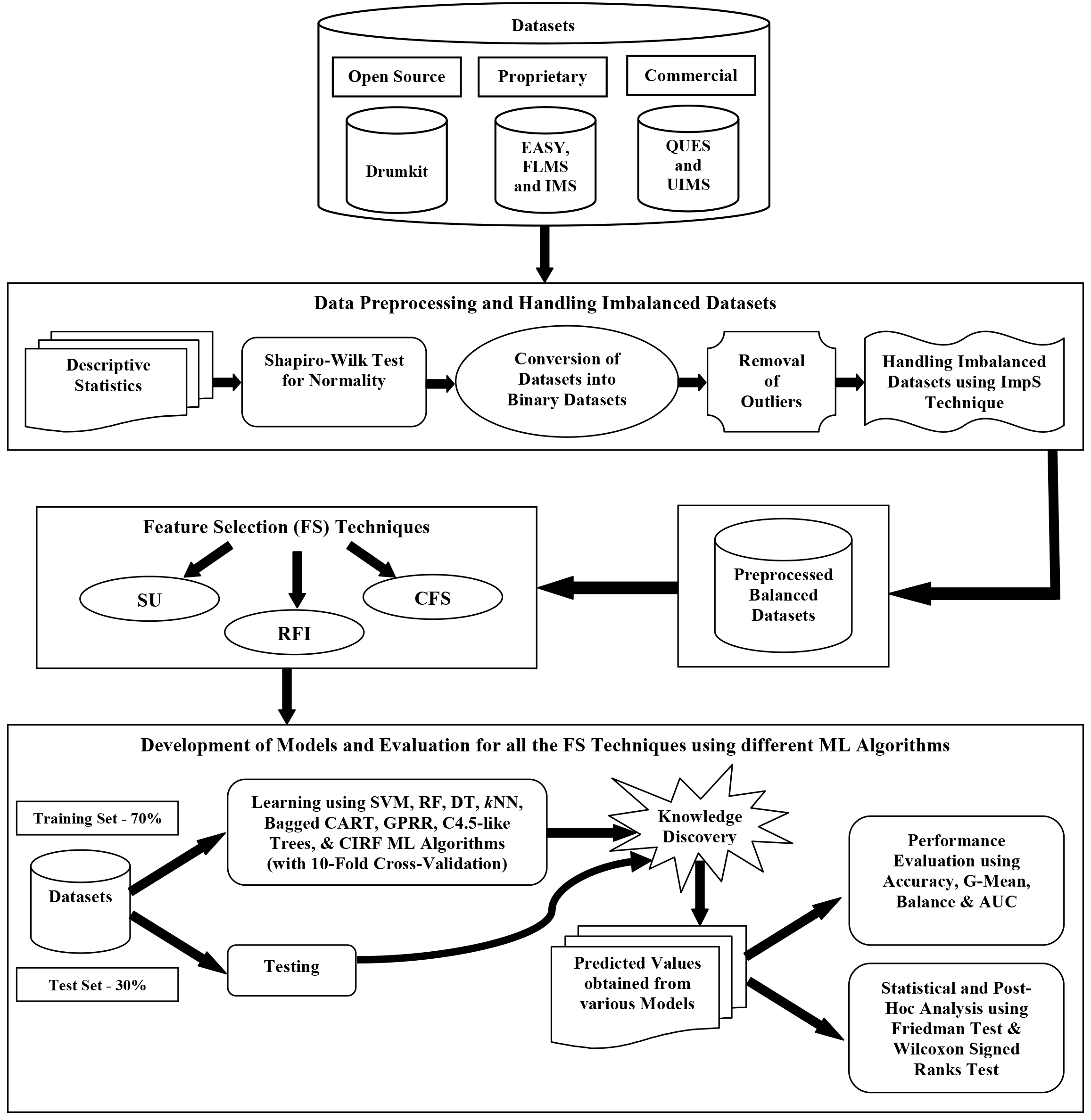

4.1 Conversion of datasets into binary datasets

Initially, as described in Section 3.2, and from Table 1, it is known that the dependent variable is Change. This variable calculates the total count of the source code lines for each data point or class that has been added, deleted, or modified in the subsequent version of the software compared to the prior version. Each addition in the source code or deletion from the code is counted as a single change whilst any modification in the existing code is counted as two changes. However, while conducting the current study, the dependent variable Change has been converted into a binary variable, known as ‘Maintainability.’ The new binary variable can take one of the two possible values of classes, i.e., L-M (1 – Low Maintainability) and H-M (0 – High Maintainability), where L-M classes require more maintenance efforts due to more number of changes in comparison to H-M classes. This conversion is done based on the criteria proposed by Dallal [20] in one of his studies attributed to the prediction of OO class maintainability using internal quality attributes. According to this criterion, for those classes where the value of Change was greater than or equal to the mean/average value of Change for all the classes taken together, the Maintainability value was set to L-M (1). On the other hand, those classes whose value of Change was less than the average value of Change were labeled as H-M (0) classes. This conversion has been done due to various reasons discussed by Morasca [62] for the unsuitability of the idea of measure for quantifying the external attributes like maintainability as described in the measurement theory. These reasons include:

(1)
Quantifying external attributes not only depends on the entity under consideration but on various additional factors as well, e.g., it would be wrong to say that the maintainability of any software product is only a function of that product itself.
(2)
Logical problems may arise when attributes are defined as per their measures due to the prior existence of attributes irrespective of how and when they have been measured. Further, the logical definition of any specific measure that intends to measure a particular attribute follows the definition of that attribute; else inconsistencies may enter while classifying attributes.
(3)
Since external attributes are affected by a number of variables apart from a particular entity, hence, they do not have any deterministic measure, which is the basic prerequisite for applying the measurement theory.

Table 4 presents the details of all the six datasets being used in this study, including the total number of data points, the number of L-M and H-M data points, the Imbalance Ratio (I-R), number of outliers, and the number of data points after outlier removal. I-R is calculated using the formula which divides the number of H-M data points by the number of L-M data points $(I-R=((H-M/L-M)*100))$ . It is evident from Table 4 that none of the six datasets being used is balanced. Rather, all of them are imbalanced datasets.

Table 4
Details of the datasets

Datasets No. of data points L-M H-M I-R No. of outliers No. of data points after outlier removal

Drumkit 91 30 61 2.03 8 83

EASY 58 21 37 1.76 6 52

FLMS 34 14 20 1.43 3 31

IMS 47 10 37 3.70 0 47

QUES 71 30 41 1.37 6 65

UIMS 39 09 30 3.33 6 33

4.2 Removal of outliers

Identification and removal of outliers from different datasets is one of the most crucial preprocessing steps for developing a useful prediction model. This is done so that the performance of the model is in no way influenced by any variability in the data points due to specific extreme values. These extreme values significantly differ from other observations in the datasets. Here, Interquartile Range (IQR) [75] filter has been used to identify and remove the outliers. IQR is a measurement of the statistical dispersion, that is equivalent to the difference in the values of the 75 ${}^{\text{th}}$ and 25 ${}^{\text{th}}$ percentiles, i.e., between the upper $(Q_{3})$ and the lower $(Q_{1})$ quartiles $(\textit{IQR}=Q_{3}-Q_{1})$ . These upper and lower bounds have been determined by subtracting 1.5 times of IQR from the first quartile or by adding 1.5 times of IQR to the third quartile. In the current context, an outlier is any data point in the datasets where any of the ten independent OO metrics, described in Section 3.2, is found to be an outlier. Proceeding in this manner, all the outliers from each of the six datasets have been found and removed, such that the predictive performance of the models being developed is least influenced by the presence of outliers. Table 4 shows the count of the outliers that have been removed for each dataset and the count of the remaining data points after removing the outliers.

4.3 Handling the imbalanced datasets

It is noticeable from Table 4 that all the six datasets being used in the current study are imbalanced in nature. Hence, it is vital to handle these imbalanced datasets for bringing about a balance between the minority and the majority classes to do away with any bias for an improved prediction. In this study, a very effective algorithm, namely, ImpS [88], has been used for handling the imbalanced datasets. This algorithm makes use of the relevance that has been provided for re-sampling the datasets to handle the imbalanced classification problem. This relevance then helps in the introduction of the copies of the most relevant examples and the removal of the least relevant ones. The ImpS algorithm applies a combination of random over-sampling and random under-sampling techniques [7] to the problematic classes as per the corresponding importance. Thus, this makes ImpS one of the best sampling techniques to handle the imbalanced datasets since it retains the best possible out of the combination of the two individual techniques.

4.4 Feature Selection (FS) techniques

While developing any prediction model, the selection of relevant features out of all the available ones becomes an essential task in enhancing the overall performance and efficiency of that model. FS reduces the initial information being fed to the model for learning while training, thereby, decreasing the execution time also. This happens since all the redundant and irrelevant features have been eliminated from the original set of features. This sub-section describes the three different FS techniques that have been used for selecting the relevant features from each dataset on an experimental basis. However, it is important to note that it is difficult to mention a single FS technique that can be considered as the best technique for FS [27, 34].

Therefore, the chosen FS techniques have been employed after a careful trial and experimentation of several FS techniques to provide the best possible results. Another reason behind choosing the below mentioned FS techniques for conducting the current study is a successful implementation of these techniques for selecting features in numerous studies in literature. For example, according to literature, SU FS technique has been applied in several different fields resulting in an effective FS for improving the predictive performance of various ML models. Jiang et al. [43] used SU FS technique to develop a hybrid FS algorithm, Kannan and Ramaraj [44] proved an effective utilization of SU technique in removing the redundant features for improving the accuracy of the classifiers, Potharaju and Sreedevi [66] proposed a novel SU-based FS technique to enhance the classification accuracy for several medical datasets, and Piao et al. [65] conducted the SU-based feature subset selection for a noteworthy classification of electricity customers. Similarly, RFI FS technique has also been successfully implemented in several prior studies. Saeys et al. [69] showed that RFI FS technique clearly outperformed other FS techniques in terms of robustness. Pan and Shen [64] revealed the importance of RFI FS in having a deep insight into the actual contribution of different features for an effective development of various predictive tools for a robust B-factor prediction. Sylvester et al. [76] effectively applied RFI FS technique for the assignment of genetic population. In one of their studies on intrusion detection, Hasan et al. [35] showcased that the RFI technique of FS is highly capable of selecting the most relevant and important features for classification. This in turn reduces the number of features and time along with an improvement in the classification accuracy. Further, if we talk about CFS FS technique, Hall and Holmes [34] assessed six different FS techniques using 15 datasets confirming the effectiveness of CFS technique over other techniques showing good results. Malhotra [58] reviewed 64 fault prediction studies (for the period 1991 to 2013) and resultantly unveiled CFS to be the most widely used FS techniques. Other studies that applied CFS technique for FS to develop effective predictive models employing various ML techniques include Hall [33], Arisholm et al. [5], and Carvalho et al. [11]. In a nutshell, the above description and studies strengthen the claim about the successful implementation of the three most effective FS techniques in the development of different prediction models employing various ML algorithms. Thus, the above three particular FS techniques, i.e., SU, RFI, and CFS have been utilized to carry out the current study.

4.4.1 Symmetrical Uncertainty (SU)

SU is an entropy-based filter [40, 85], which is derived by normalizing the mutual information to the entropies of either the feature values, or the feature values and the target classes. Mutual information here refers to the measure of the difference between the distribution of the feature values and the target classes from statistical independence. This estimates the correlation between the feature values, or the feature values and the target classes in a non-linear manner. SU has prominently been used for evaluating the relevance of features for classification. SU is measured as follows:

$\displaystyle\textit{IG}\left(A|B\right)=E\left(A\right)-E\left(A|B\right)$ (2) $\displaystyle\textit{SU}\left(A,B\right)=2\times\frac{IG\left(A|B\right)}{E% \left(A\right)+E\left(B\right)}$ (3)

where, $E(A)$ and $E(B)$ represent the entropy of the features $A$ and $B$ , respectively, and $\textit{IG}(A|B)$ represents the information gain of $A$ on observing $B$ .

4.4.2 Random Forest Filter (RFI)

RFI [85] uses the RF algorithm to find the weights of various features. RF consists of a number of decision trees that are built from a random extraction of different observations in a dataset, along with a random extraction of various features. Each and every tree is not necessarily exposed to all the observations or features at the same time, which ensures that the trees are sufficiently de-correlated and, hence, less susceptible to the problem of over-fitting. Here, every tree is a series of questions (each question represents a node) in yes-no form, formed on the basis of an individual or a blend of various features. The tree is further divided into two branches at every subsequent node, where each branch consists of all those observations that are similar to each other but not so similar to the ones hosted by the other branch. Thus, the relevance of each and every feature is decided based on the purity of the corresponding branch. Generally, in RF, the features selected by the tree at the top are considered to be more important than that of those selected by the end nodes.

4.4.3 Correlation-based Feature Selection (CFS)

CFS [40, 85] algorithm uses the measures of correlation and entropy to find a subset of the relevant features. CFS selects the features in a way such that the selected features are highly correlated to the dependent variable and have the least possible correlation amongst each other. Further, CFS uses a heuristic-based evaluation function based on the values of correlations for the ranking of features. Different subsets of feature vectors that are in correlation with the dependent variable, but independent of each other are evaluated using this function. According to the CFS algorithm, features showing a low correlation with the dependent variable are irrelevant, and hence, they should be ignored. Typically, CFS sometimes even eliminates over half of the total features. A subset $S$ of ‘ $m$ ’ features is assessed using the following criterion:

$\displaystyle M_{S_{m}}=\frac{m\bar{p}_{cf}}{\sqrt{m+m\left(m-1\right)\bar{p}_% {ff}}}$ (4)

where $M_{S_{m}}$ represents the assessment for a subset of $S$ containing $m$ features, $\bar{p}_{cf}$ represents the value of the average correlation between the features and the labels of the class, and $\bar{p}_{ff}$ represents the value of the average correlation between the two features.

4.5 Machine Learning (ML) techniques

Once the relevant features are selected from all the datasets using each of the FS techniques, these datasets are divided into a $70-30$ train-test ratio for the development of various prediction models. Eight different ML algorithms have been used for developing these models. Further, $10$ -fold cross-validation has been performed on the train set while training the models to reduce the bias in validation, leaving test set to be used only once. In cross-validation technique, all the data points of a particular dataset are divided into $10$ equal-sized partitions, where, at a time, $9$ out of the $10$ partitions are used for the task of training while the remaining $10^{\text{th}}$ partition is utilized for validation. The stated process is iterated $10$ times until each of the $10$ partitions has been used for validation once. A concern about this approach, where the datasets are first split into train and test sets followed by passing of train set for $10$ -fold cross-validation is the possibility of biasness towards the data present in train set. However, with respect to this concern, it is hoped that the random split that has been used for creating the train set is not at all biased in any way. It is also hoped that this data is representative enough, such that any other sufficiently large subgroup of data is also representative. The current section now describes various ML algorithms that have been used in the current study. All the algorithms have been implemented in “RStudio Version 1.2.5042 [68] using R Version 4.0.0 [87]”.

SVM is a supervised ML algorithm put forth by Vapnik [14] along with his colleagues at At&T Bell Laboratories. It can be used for the analysis of both classification and regression problems. The principal objective of SVM is to identify a hyperplane in an $q$ -dimensional space, where ‘ $q$ ’ represents the number of features, which classifies the observations distinctly. A hyperplane is nothing but a decision boundary which helps in the classification of various data points. Points that fall on either side of the hyperplane are considered belonging to different classes. However, the number of features decides about what dimension a hyperplane should take. While separating the two classes, there are many possibilities for choosing a hyperplane. Eventually, the plane having the maximum margin or distance between the data points of the two different classes is chosen. Further, SVM can carry out both linear and non-linear classification, where non-linear classification is characterized by the kernel trick. The most extensively used kernels with SVM include the linear, polynomial, and radial basis function kernels. Here, ‘radial’ kernel has been used.

RF is another supervised ML ensemble for classification and regression problems [9] consisting of multiple DTs. In RF, every individual tree generates a class prediction where the class having the majority of votes becomes the final prediction. The strength of RF lies in the fact that a number of uncorrelated trees operate collectively to outperform several individual trees and protect one another from the individual errors. One of the prerequisites of RF for better performance is that there should be a low correlation among the prediction of individual trees. Therefore, RF tries to build a forest of trees that is uncorrelated in nature using feature randomness and bagging (bootstrap aggregation) while creating individual trees such that the collective prediction is always more accurate as compared to individual trees. Finally, RF results in ensemble predictions by integrating the decisions of each DT, which are indeed more accurate than any of the individual predictions.

DT(rpart) [77] method is a popular, exploratory and widely used statistical tool for solving many classification and regression problems whose primary objective is to bring down the dissimilarity existing in the terminal nodes of the DT to a minimum. It is generally used for dichotomous outcomes such that the assumption of linearity can be avoided. In this method, a DT is built by repeated division/splitting of a dataset, i.e., the whole population into various subsets based on some rules or descriptors that differentiate between different types of data points. This method is recursive since each subset may further be split for an unspecified number of times until it reaches a stopping criterion to terminate the splitting process and receive the final predicted class or value. The predictions made using DT(rpart) can be more accurate as it ensures varying prioritization of the misclassifications for creating a decision rule having more specificity or sensitivity.

$k$ NN algorithm proposed by Thomas Cover [17, 79] is another non-parametric supervised ML algorithm utilized for both the regression and the classification predictive problems producing competitive results. It is also known as a lazy learning algorithm since it makes use of all the available data for classification as there is no special training phase. $k$ NN classifies different data points based on some similarity. Test data is used for making an educated guess so as to decide which class should an unclassified point be classified to. $k$ NN is implemented by transforming the data points into their respective mathematical values or feature vectors and then finding the distance, such as the Euclidean distance between the values of these data points and the test data. After this, the probability of test data being similar to these data points is found, and then this test data is classified into the class of those data points with which it shares the highest probability. In other words, the test data is assigned to the class, which is the most common class amongst the ‘ $k$ ’ neighbors in its vicinity, where $k$ is any integer. In $k$ NN, every instance votes for its class and the class having the majority of votes is considered the final prediction.

Bagged CART combines bagging with the CART algorithm to develop an integrated algorithm for classification since the CART algorithm lacks stability in training and prediction when used individually. Bagged CART not only includes the simplicity of the CART algorithm but, in turn, enhances the reliability and accuracy of the classification. Breiman [19] proposed the CART, i.e., the Classification and Regression Trees classification algorithm in 1984. In CART, non-parametric methods are used to determine the relationship between the multiple layers of data and to meet the classification goals through the construction of binary graphics. However, CART is an unstable algorithm.

Further, a few years later, it was pointed out by Breiman [8] that bagging can improvise the predictive performance of the weak and unstable learning algorithms significantly by iterating over several different versions of a particular predictor to obtain an aggregated predictor. This aggregation then averages out or makes a plurality vote over all the versions during prediction. Hence, the bagging algorithm has been used with the CART algorithm for an increased optimizing ability of the CART algorithm.

GPRR model was developed by O’Hagan and others [57] in the seventies. Gaussian Process (GP) is again a non-parametric, generic and supervised method of classification, which is based on Bayesian methodology. It is based on a prior assumption of distribution on the underlying density of the probabilities guaranteeing the smoothness property. The classification providing a good fit for the observed values is considered to be the final classification. GP is a distribution of probability over possible functions. It is advantageous as the observations are interpolated by the prediction. The prediction is Gaussian or probabilistic in nature, such that the empirical confidence intervals may be computed for deciding if the prediction should be refit in the region of interest and is versatile in terms of the kernels used. Kernels or the covariance functions play a crucial role in ascertaining the prior and posterior shape of the GP. They do so by encoding the assumptions of the learning function by combining the defined similarity of the two data points with an assumption that two similar data points are supposed to have similar targets. Here, Radial-Basis Function (RBF) kernel, otherwise known to be the squared exponential kernel has been used. RBF is a stationary kernel.

C4.5-like trees is an algorithm propounded by Ross Quinlan [70], which is applied for generating a DT. It is an enhancement to Quinlan’s ID3 algorithm. C4.5 is otherwise known as a statistical classifier since the DTs generated by C4.5 are used for classification. It uses an information entropy concept for building the DTs from a given set of already classified training data. At each tree node, C4.5 works by selecting such attributes of the dataset that split the whole set of observations into various subsets in the most effective manner enriched in one or the other class. The splitting is done based on the criterion of normalized Information Gain (IG), i.e., the difference in entropy and the attribute having the highest IG is chosen for making the decision. After this, the C4.5 algorithm recurrently iterates over the partitioned subsets.

CIRF is an implementation of RF [9] and the bagging ensemble models which use Conditional Inference (CI) trees [38] in the form of base learners. Unlike RF, where predictions are averaged out directly; in CIRF, aggregation is done by finding out the average of the weights of the observations extracted from each and every tree. Generally, CI trees grow in a usual manner on the bootstrap samples or the sub-samples having only a subset of attributes being available for the split at each node. After this, a suitable and weighted average of the responses that have been observed is constructed for the predictions [37]. Further, the CI trees apply the significance tests to determine the split attributes and the split points.

4.6 Performance evaluation measures

This section talks about various performance measures that have been used to estimate the performance of different prediction models being developed in the current study. Precisely, one traditional evaluation measure, i.e., Accuracy along with three other robust measures, viz., G-Mean, Balance, and AUC have been used in this study to measure the performance. The use of all the above three robust measures in determining the performance of the predictive models has already been advocated in various prior studies [36, 49, 53, 73].

All the above evaluation measures have been derived in accordance with the confusion matrix [56]. A confusion matrix for the concerned study has been provided in Table 5 representing two different classes, i.e., H-M (0), the majority class, and L-M (1), the minority class. Here, H-M is relative to the positive class, whereas L-M symbolizes the negative class.

Table 5
Confusion matrix

	Predicted Positive	Predicted Negative
Actual Positive (H-M)	True Positive (TP)	False Negative (FN)
Actual Negative (L-M)	False Positive (FP)	True Negative (TN)

Based on the confusion matrix, various performance measures are described as follows:

(1)

Accuracy computes the percentage of the correctly predicted classes, including both the positive and the negative classes using the following formula:

$\displaystyle\textit{Accuracy}=\frac{\textit{TP}+\textit{TN}}{\textit{TP}+% \textit{FP}+\textit{FN}+\textit{TN}}*100$ (5)

(2)

G-Mean symbolizes the geometric mean of the sensitivity ( $\textit{TPR}=\textit{True Positive Rate}$ ) and the specificity ( $\textit{TNR}=\textit{True Negative Rate}$ ), which balances the accuracies of both, the majority and the minority classes, unlike the traditional Accuracy metric.

$\displaystyle\textit{G-Mean}=\sqrt{\textit{TPR*TNR}},$ (6)

$\displaystyle\textit{TPR}=\sqrt{\frac{\textit{TP}}{\textit{TP}+\textit{FN}}}% \quad\text{and}\quad\textit{TNR}=\sqrt{\frac{\textit{TN}}{\textit{TN}+\textit{% FP}}}$ (7)

(3)

Balance measure computes the Euclidean distance between a particular pair, i.e., (Recall or TPR, FPR or False Positive Rate) to a pair having the optimum value of (Recall, FPR). The optimum value of Recall $=$ 1 and $\textit{FPR}=$ 0.

$\displaystyle\textit{Balance}=1-\sqrt{\frac{(0-\textit{FPR})^{2}+(1-\textit{% TPR})^{2}}{2}},$ (8) $\displaystyle\textit{FPR}=\sqrt{\frac{\textit{FP}}{\textit{FP}+\textit{TN}}}$ (9)

(4)

AUC is another significant measure to evaluate the performance of the predictive models. It represents the area under the ROC (Receiver Operating Characteristic) curve between FPR (1-specificity or $1-\textit{TNR}$ ) values depicted on the $x$ -axis, and TPR (recall) values depicted on the $y$ -axis. A prediction model having a higher value of AUC gets qualified to be considered as a favourable model.

4.7 Statistical and post-hoc analysis

Once the results have been obtained for various prediction models, it is essential to perform some statistical tests such that these results get support for strengthening the conclusions of the current study through statistical analysis. In this study, two non-parametric tests, namely, the Friedman Test followed by the Wilcoxon Signed Ranks Test for post-hoc analysis have been used.

Table 6
Table for Feature Selection (FS)

Number and names of features/OO metrics selected
ML technique	FS technique used	Drumkit	EASY	FLMS	IMS	QUES	UIMS
SVM	1. SU	7 (dit, noc, mpc, rfc, lcom, dac, wmc)	5 (dit, noc, mpc, rfc, lcom)	6 (size1, dit, noc, mpc, rfc, lcom)	5 (dit, noc, mpc,rfc, lcom)	3 (mpc, dit, rfc)	3 (dit, noc, mpc)
	2. RFI	7 (size1, size2, rfc, dit, wmc, nom, mpc)	3 (lcom, size2, size1)	7 (size1, lcom, dac,mpc, wmc, nom, size2)	3 (noc, rfc, size2)	3 (size1, mpc, dac)	5 (size2, wmc, size1,dac, mpc)
	3. CFS	3 (dac, size2, size1)	4 (mpc, lcom, size2, size1)	4 (dit, rfc, lcom, dac)	2 (noc, lcom)	1 (size1)	2 (lcom, wmc)
RF	1. SU	6 (dit, noc, mpc, rfc, lcom, dac)	6 (dit, noc, mpc, rfc, lcom, dac)	7 (size1, dit, noc, mpc, rfc, lcom, dac)	3 (dit, noc, mpc)	5 (mpc, dit, rfc, lcom, dac)	4 (dit, noc, mpc, rfc)
	2. RFI	5 (size1, size2, rfc, dit, wmc)	4 (lcom, size2, size1, dac)	5 (size1, lcom, dac, mpc, wmc)	5 (noc, rfc, size2, dac, wmc)	3 (size1, mpc, dac)	3 (size2, wmc, size1)
	3. CFS	3 (dac, size2, size1)	4 (mpc, lcom, size2, size1)	4 (dit, rfc, lcom, dac)	2 (noc, lcom)	1 (size1)	2 (lcom, wmc)
DT (rpart)	1. SU	10 (dit, noc, mpc, rfc, lcom, dac, wmc, nom, size2, size1)	1 (dit)	5 (szie1, dit, noc, mpc, rfc)	2 (dit, noc)	4 (mpc, dit, rfc, lcom)	4 (dit, noc, mpc, rfc)
	2. RFI	7 (size1, size2, rfc, dit, wmc, nom, mpc)	1 (lcom)	7 (size1, lcom, dac, mpc, wmc, nom, size2)	5 (noc, rfc, size2, dac, wmc)	2 (size1, mpc)	1 (size2)
	3. CFS	3 (dac, size2, size1)	4 (mpc, lcom, size2, size1)	4 (dit, rfc, lcom, dac)	2 (noc, lcom)	1 (size1)	2 (lcom, wmc)
kNN	1. SU	4 (dit, noc, mpc, rfc)	10 (dit, noc, mpc, rfc, lcom, dac, wmc, nom, size2, size1)	6 (szie1, dit, noc, mpc, rfc, lcom)	1 (dit, noc, mpc)	2 (mpc, dit)	4 (dit, noc, mpc, rfc)
	2. RFI	7 (size1, size2, rfc, dit, wmc, nom, mpc)	7 (lcom, size2, size1, dac, mpc, noc, wmc)	5 (size1, lcom, dac, mpc, wmc)	4 (noc, rfc, size2, dac)	4 (size1, mpc, dac, rfc)	3 (size2, wmc, size1)
	3. CFS	3 (dac, size2, size1)	4 (mpc, lcom, size2, size1)	4 (dit, rfc, lcom, dac)	2 (noc, lcom)	1 (size1)	2 (lcom, wmc)
Bagged CART	1. SU	5 (dit, noc, mpc, rfc, lcom)	6 (dit, noc, mpc, rfc, lcom, dac)	4 (size1, dit, noc, mpc)	3 (dit, noc, mpc)	4 (dit, mpc, rfc, lcom)	3 (dit, noc, mpc)
	2. RFI	6 (size1, wmc, size2, rfc, nom, mpc)	4 (lcom, size2, size1, dac)	3 (size1, lcom, dac)	5 (noc, rfc, size2, dac, wmc)	6 (size1, mpc, dac, wmc, rfc, lcom)	4 (mpc, size1, wmc, size2)
	3. CFS	3 (dac, size2, size1)	4 (mpc, lcom, size2, size1)	4 (dit, rfc, lcom, dac)	2 (noc, lcom)	1 (size1)	2 (lcom, wmc)

Table 6, continued
Number and names of features/OO metrics selected
ML technique	FS technique used	Drumkit	EASY	FLMS	IMS	QUES	UIMS
GPRR	1. SU	10 (dit, noc, mpc, rfc, lcom, dac, wmc, nom, size2, size1)	1 (dit, noc, mpc)	3 (size1, dit, noc)	8 (dit, noc, mpc, rfc, lcom, dac, wmc, nom)	4 (dit, mpc, rfc, lcom)	3 (dit, noc, mpc)
	2. RFI	3 (size1, size2, rfc)	2 (lcom, size2)	3 (size1, lcom, dac)	6 (noc, rfc, size2, dac, wmc, lcom)	3 (size1, mpc, dac)	6 (size2, wmc, size1, dac, mpc, dit)
	3. CFS	3 (dac, size2, size1)	4 (mpc, lcom, size2, size1)	4 (dit, rfc, lcom, dac)	2 (noc, lcom)	1 (size1)	2 (lcom, wmc)
C4.5-like Trees	1. SU	4 (dit, noc, mpc, rfc)	8 (dit, noc, mpc, rfc, lcom, dac, wmc, nom)	3 (size1, dit, noc)	2 (dit, noc)	2 (dit, mpc)	6 (dit, noc, mpc, rfc, lcom, dac)
	2. RFI	5 (size1, size2, rfc, dit, wmc)	4 (lcom, size2, size1, dac)	3 (size1, lcom, dac)	4 (noc, rfc, size2, dac)	2 (size1, mpc)	3 (size2, wmc, size1)
	3. CFS	3 (dac, size2, size1)	4 (mpc, lcom, size2, size1)	4 (dit, rfc, lcom, dac)	2 (noc, lcom)	1 (size1)	2 (lcom, wmc)
CIRF	1. SU	7 (dit, noc, mpc, rfc, lcom, dac, wmc)	6 (dit, noc, mpc, rfc, lcom, dac)	4 (size1, dit, noc, mpc)	9 (dit, noc, mpc, rfc, lcom, dac, wmc, nom, size2)	2 (dit, mpc)	4 (dit, noc, mpc, rfc)
	2. RFI	6 (size1, size2, rfc, dit, wmc, nom)	3 (lcom, size2, size1)	4 (size1, lcom, dac, mpc)	4 (noc, rfc, size2, dac)	3 (size1, mpc, dac)	1 (size2)
	3. CFS	3 (dac, size2, size1)	4 (mpc, lcom, size2, size1)	4 (dit, rfc, lcom, dac)	2 (noc, lcom)	1 (size1)	2 (lcom, wmc)

Friedman Test [84] has been used to advocate for any significant difference among the performances of the different prediction models that have been developed in this study using different FS techniques for each dataset employing Accuracy, G-Mean, Balance and AUC performance measures (RQ2). Further, a mean rank is assigned to different FS techniques for each and every dataset depending on the four different performance measures mentioned above. The lower the rank of the FS technique, the better is that technique.

Friedman test distributes the test statistic as per the Chi-Square distribution having ‘ $r-1$ ’ degrees of freedom, where ‘ $r$ ’ represents the number of FS techniques being compared. While testing the hypothesis in the Friedman test, a specific $p$ -value, or the level of significance ( $\alpha$ ) is stated, which is equal to 0.05 here ( $\alpha=$ 0.05).

Once it is known that the results on performing the Friedman test are significant, then the Wilcoxon Signed Ranks test should also be performed to ascertain pair-wise differences among different FS techniques.

Wilcoxon Signed Ranks Test [84] finds the differences amongst the various possible pairs of different FS techniques for comparison for each dataset. Further, according to the absolute values of the calculated differences, ranks are allocated to them. In this study, the Wilcoxon test has been performed with Bonferroni correction for handling the family-wise error and compensating for the inflation of Type I error. Here also, the level of significance is taken to be 0.05, i.e., $\alpha=$ 0.05. Bonferroni adjustment is made such that if ‘ $s$ ’ Wilcoxon post-hoc tests have been performed after the Friedman test, the value of $\alpha$ is adjusted to $\alpha/s$ .

Table 7

Results for Accuracy using different FS techniques

ML technique	Drumkit				ML technique	IMS
	No FS	SU	RFI	CFS		No FS	SU	RFI	CFS
SVM	64.00	84.62	80.77	73.08	SVM	86.67	86.67	86.67	80.00
RF	60.00	88.46	76.92	73.08	RF	93.00	93.33	86.67	93.33
DT (rpart)	72.00	84.62	84.62	84.62	DT (rpart)	86.67	66.67	66.67	66.67
kNN	76.00	88.46	69.23	61.54	kNN	86.67	80.00	80.00	66.67
Bagged CART	64.00	88.46	76.92	73.08	Bagged CART	73.33	93.33	93.33	93.33
GPRR	68.00	76.92	84.62	84.62	GPRR	86.67	86.67	86.67	86.67
C4.5-like Trees	60.00	80.77	84.62	61.54	C4.5-like Trees	86.67	86.67	93.33	86.67
CIRF	64.00	84.62	88.46	76.92	CIRF	86.67	80.00	80.00	66.67
ML technique	EASY				ML technique	QUES
	No FS	SU	RFI	CFS		No FS	SU	RFI	CFS
SVM	62.50	93.75	93.75	93.75	SVM	55.00	100.00	100.00	90.00
RF	75.00	87.50	93.75	75.00	RF	90.00	95.00	95.00	85.00
DT (rpart)	62.50	75.00	75.00	62.50	DT (rpart)	70.00	80.00	80.00	60.00
kNN	75.00	75.00	75.00	56.25	kNN	60.00	75.00	65.00	65.00
Bagged CART	81.25	93.75	81.25	75.00	Bagged CART	85.00	80.00	80.00	45.00
GPRR	68.75	87.50	68.75	62.50	GPRR	85.00	100.00	95.00	45.00
C4.5-like Trees	62.50	81.25	87.50	62.50	C4.5-like Trees	75.00	85.00	65.00	40.00
CIRF	62.50	81.25	68.75	62.50	CIRF	70.00	75.00	60.00	40.00
ML technique	FLMS				ML technique	UIMS
	No FS	SU	RFI	CFS		No FS	SU	RFI	CFS
SVM	70.00	100.00	100.00	80.00	SVM	80.00	100.00	100.00	90.00
RF	70.00	100.00	100.00	70.00	RF	80.00	90.00	90.00	100.00
DT (rpart)	70.00	100.00	100.00	70.00	DT (rpart)	80.00	90.00	90.00	70.00
kNN	60.00	100.00	100.00	80.00	kNN	80.00	90.00	90.00	70.00
Bagged CART	90.00	100.00	100.00	80.00	Bagged CART	80.00	90.00	70.00	80.00
GPRR	60.00	100.00	100.00	90.00	GPRR	80.00	80.00	90.00	70.00
C4.5-like Trees	50.00	100.00	100.00	80.00	C4.5-like Trees	80.00	90.00	90.00	70.00
CIRF	50.00	100.00	100.00	80.00	CIRF	80.00	90.00	90.00	70.00

Table 8

Results for G-Mean using different FS techniques

ML technique	Drumkit				ML technique	IMS
	No FS	SU	RFI	CFS		No FS	SU	RFI	CFS
SVM	0.00	0.77	0.71	0.66	SVM	0.00	0.87	0.87	0.80
RF	0.42	0.89	0.79	0.75	RF	0.71	0.94	0.87	0.94
DT (rpart)	0.67	0.86	0.86	0.86	DT (rpart)	0.00	0.65	0.65	0.65
kNN	0.65	0.90	0.71	0.63	kNN	0.00	0.79	0.79	0.65
Bagged CART	0.43	0.88	0.77	0.75	Bagged CART	0.00	0.94	0.94	0.94
GPRR	0.45	0.77	0.87	0.86	GPRR	0.00	0.87	0.87	0.87
C4.5-like Trees	0.42	0.82	0.87	0.63	C4.5-like Trees	0.00	0.87	0.94	0.87
CIRF	0.44	0.84	0.90	0.79	CIRF	0.00	0.79	0.79	0.65
ML technique	EASY				ML technique	QUES
	No FS	SU	RFI	CFS		No FS	SU	RFI	CFS
SVM	0.00	0.94	0.94	0.94	SVM	0.00	1.00	1.00	0.90
RF	0.58	0.87	0.93	0.65	RF	0.88	0.95	0.95	0.85
DT (rpart)	0.00	0.75	0.75	0.62	DT (rpart)	0.67	0.80	0.80	0.60
kNN	0.58	0.71	0.71	0.56	kNN	0.52	0.74	0.64	0.65
Bagged CART	0.77	0.93	0.80	0.65	Bagged CART	0.85	0.81	0.81	0.49
GPRR	0.41	0.87	0.69	0.58	GPRR	0.85	1.00	0.96	0.49
C4.5-like Trees	0.39	0.76	0.87	0.62	C4.5-like Trees	0.80	0.89	0.69	0.42
CIRF	0.00	0.82	0.67	0.62	CIRF	0.73	0.72	0.65	0.42
ML technique	FLMS				ML technique	UIMS
	No FS	SU	RFI	CFS		No FS	SU	RFI	CFS
SVM	0.00	1.00	1.00	0.77	SVM	0.00	1.00	1.00	0.91
RF	0.76	1.00	1.00	0.69	RF	0.00	0.87	0.87	1.00
DT (rpart)	0.00	1.00	1.00	0.69	DT (rpart)	0.00	0.87	0.87	0.65
kNN	0.62	1.00	1.00	0.77	kNN	0.00	0.87	0.87	0.65
Bagged CART	0.93	1.00	1.00	0.77	Bagged CART	0.00	0.89	0.63	0.77
GPRR	0.62	1.00	1.00	0.89	GPRR	0.00	0.79	0.87	0.65
C4.5-like Trees	0.53	1.00	1.00	0.77	C4.5-like Trees	0.00	0.87	0.87	0.65
CIRF	0.53	1.00	1.00	0.77	CIRF	0.00	0.87	0.87	0.65

Table 9

Results for Balance using different FS techniques

ML technique	Drumkit				ML technique	IMS
	No FS	SU	RFI	CFS		No FS	SU	RFI	CFS
SVM	0.29	0.72	0.65	0.64	SVM	0.29	0.82	0.82	0.80
RF	0.43	0.89	0.77	0.73	RF	0.65	0.91	0.87	0.91
DT (rpart)	0.66	0.85	0.85	0.85	DT (rpart)	0.29	0.63	0.63	0.63
kNN	0.60	0.87	0.65	0.60	kNN	0.29	0.73	0.78	0.63
Bagged CART	0.43	0.88	0.76	0.73	Bagged CART	0.28	0.91	0.91	0.91
GPRR	0.43	0.77	0.82	0.85	GPRR	0.29	0.87	0.87	0.82
C4.5-like Trees	0.43	0.81	0.82	0.62	C4.5-like Trees	0.29	0.87	0.91	0.87
CIRF	0.44	0.83	0.87	0.73	CIRF	0.29	0.73	0.73	0.63
ML technique	EASY				ML technique	QUES
	No FS	SU	RFI	CFS		No FS	SU	RFI	CFS
SVM	0.29	0.92	0.92	0.92	SVM	0.29	1.00	1.00	0.87
RF	0.53	0.87	0.90	0.60	RF	0.84	0.94	0.94	0.81
DT (rpart)	0.29	0.69	0.69	0.62	DT (rpart)	0.66	0.74	0.74	0.60
kNN	0.53	0.69	0.69	0.56	kNN	0.51	0.68	0.61	0.65
Bagged CART	0.75	0.90	0.78	0.60	Bagged CART	0.84	0.81	0.81	0.49
GPRR	0.41	0.87	0.69	0.57	GPRR	0.84	1.00	0.95	0.48
C4.5-like Trees	0.41	0.70	0.87	0.62	C4.5-like Trees	0.75	0.85	0.67	0.43
CIRF	0.29	0.81	0.66	0.62	CIRF	0.72	0.72	0.63	0.43
ML technique	FLMS				ML technique	UIMS
	No FS	SU	RFI	CFS		No FS	SU	RFI	CFS
SVM	0.29	1.00	1.00	0.72	SVM	0.29	1.00	1.00	0.88
RF	0.70	1.00	1.00	0.68	RF	0.29	0.82	0.82	1.00
DT (rpart)	0.29	1.00	1.00	0.68	DT (rpart)	0.29	0.82	0.82	0.63
kNN	0.62	1.00	1.00	0.72	kNN	0.29	0.82	0.82	0.63
Bagged CART	0.90	1.00	1.00	0.72	Bagged CART	0.29	0.86	0.58	0.72
GPRR	0.62	1.00	1.00	0.86	GPRR	0.29	0.79	0.82	0.63
C4.5-like Trees	0.49	1.00	1.00	0.72	C4.5-like Trees	0.29	0.82	0.82	0.63
CIRF	0.49	1.00	1.00	0.72	CIRF	0.29	0.82	0.82	0.63

Table 10

Results for AUC using different FS techniques

ML technique	Drumkit				ML technique	IMS
	No FS	SU	RFI	CFS		No FS	SU	RFI	CFS
SVM	0.50	0.80	0.75	0.69	SVM	0.50	0.88	0.88	0.80
RF	0.52	0.89	0.79	0.76	RF	0.75	0.94	0.87	0.94
DT (rpart)	0.68	0.86	0.86	0.86	DT (rpart)	0.50	0.68	0.68	0.68
kNN	0.69	0.91	0.75	0.67	kNN	0.50	0.81	0.79	0.68
Bagged CART	0.57	0.88	0.77	0.76	Bagged CART	0.42	0.94	0.94	0.94
GPRR	0.60	0.78	0.88	0.86	GPRR	0.50	0.87	0.87	0.88
C4.5-like Trees	0.52	0.83	0.88	0.63	C4.5-like Trees	0.50	0.87	0.94	0.87
CIRF	0.55	0.84	0.91	0.81	CIRF	0.50	0.81	0.81	0.68
ML technique	EASY				ML technique	QUES
	No FS	SU	RFI	CFS		No FS	SU	RFI	CFS
SVM	0.50	0.94	0.94	0.94	SVM	0.50	1.00	1.00	0.91
RF	0.67	0.87	0.93	0.71	RF	0.89	0.95	0.95	0.86
DT (rpart)	0.50	0.78	0.78	0.62	DT (rpart)	0.69	0.82	0.82	0.61
kNN	0.67	0.73	0.73	0.56	kNN	0.58	0.77	0.67	0.65
Bagged CART	0.78	0.93	0.80	0.71	Bagged CART	0.85	0.81	0.81	0.51
GPRR	0.58	0.87	0.69	0.60	GPRR	0.85	1.00	0.96	0.56
C4.5-like Trees	0.53	0.79	0.87	0.62	C4.5-like Trees	0.82	0.89	0.70	0.52
CIRF	0.50	0.82	0.67	0.62	CIRF	0.74	0.73	0.67	0.52
ML technique	FLMS				ML technique	UIMS
	No FS	SU	RFI	CFS		No FS	SU	RFI	CFS
SVM	0.50	1.00	1.00	0.80	SVM	0.50	1.00	1.00	0.92
RF	0.79	1.00	1.00	0.70	RF	0.50	0.88	0.88	1.00
DT (rpart)	0.50	1.00	1.00	0.70	DT (rpart)	0.50	0.88	0.88	0.67
kNN	0.62	1.00	1.00	0.80	kNN	0.50	0.88	0.88	0.67
Bagged CART	0.93	1.00	1.00	0.80	Bagged CART	0.50	0.90	0.70	0.80
GPRR	0.62	1.00	1.00	0.90	GPRR	0.50	0.79	0.88	0.67
C4.5-like Trees	0.64	1.00	1.00	0.80	C4.5-like Trees	0.50	0.88	0.88	0.67
CIRF	0.64	1.00	1.00	0.80	CIRF	0.50	0.88	0.88	0.67

5. Results and discussions

The current section presents the results of this study, along with extensive analysis. The study has been performed on six different datasets after their preprocessing, including converting these datasets into binary, removing outliers, and balancing the imbalanced datasets using the ImpS technique. The preprocessing has been followed by FS with the help of three FS techniques, namely, SU, RFI and CFS. Afterward, the resultant datasets have been used for developing the prediction models by dividing them into a $70-30$ train-test ratio using each of the above three FS techniques for each dataset and eight different ML algorithms with $10$ -fold cross-validation. Further, Accuracy, G-Mean, Balance and AUC measures have been used for estimating and analyzing the performance of the models. Lastly, a statistical and post-hoc analysis has also been done for analyzing and comparing the results using the Friedman test and the Wilcoxon Signed Ranks test.

5.1 Feature Selection (FS) results

This study implements three different FS techniques, described in Section 4.4, for choosing the relevant features from each of the six datasets. Table 6 provides a complete list of features or the OO metrics that have been selected using SU, RFI and CFS techniques of FS for developing the prediction models for all the datasets using different ML algorithms.

It is observable from Table 6 that each FS technique selects an entirely different set of OO metrics both in terms of names and numbers depending on the dataset and the ML technique being used at a particular instance. However, the effect of all these FS techniques on the performance of various prediction models has been stated and explained in the subsequent sections with the help of different performance measures.

5.2 Evaluation and discussion of results using different FS techniques and ML algorithms with 10-fold cross-validation

This sub-section answers the first RQ formulated in this study, i.e., RQ1: Whether the performance of different ML algorithms used in this study improves markedly by using various FS techniques for predicting software maintainability?

Several prediction models have been developed for six different datasets using three FS techniques and eight ML algorithms for answering the above RQ. All the ML algorithms have been implemented using the 10-fold cross-validation while training. Since, for each of the 6 datasets, a total of 4 FS techniques (3 FS techniques $+$ 1 No FS case) along with 8 different ML have been employed in this study, therefore, resultantly 6 $\times$ 4 $\times$ 8 $=$ 192 predictive models have been developed for conducting the current work. The performance of all the developed predictive models has been assessed using Accuracy, G-Mean, Balance and AUC as the performance evaluation measures. Tables 7–10 provide the values of various performance measures as obtained by applying eight ML algorithms on six datasets using three different FS techniques and the case where no FS is performed.

As per Table 7, for all the datasets, the values of Accuracy in some cases are better when no FS technique has been used as compared to the cases where some or the other FS has been applied, especially in case of IMS, QUES, and UIMS datasets. Further, the SMP models that have been built with FLMS, Drumkit and EASY datasets still performed well with FS in terms of Accuracy since the values of Accuracy using FS techniques are better than the case when no FS has been done in majority cases.

Figure 2.

Median values obtained for (a) Accuracy; (b) G-Mean; (c) Balance; and (d) AUC for all the six datasets before and after using FS techniques.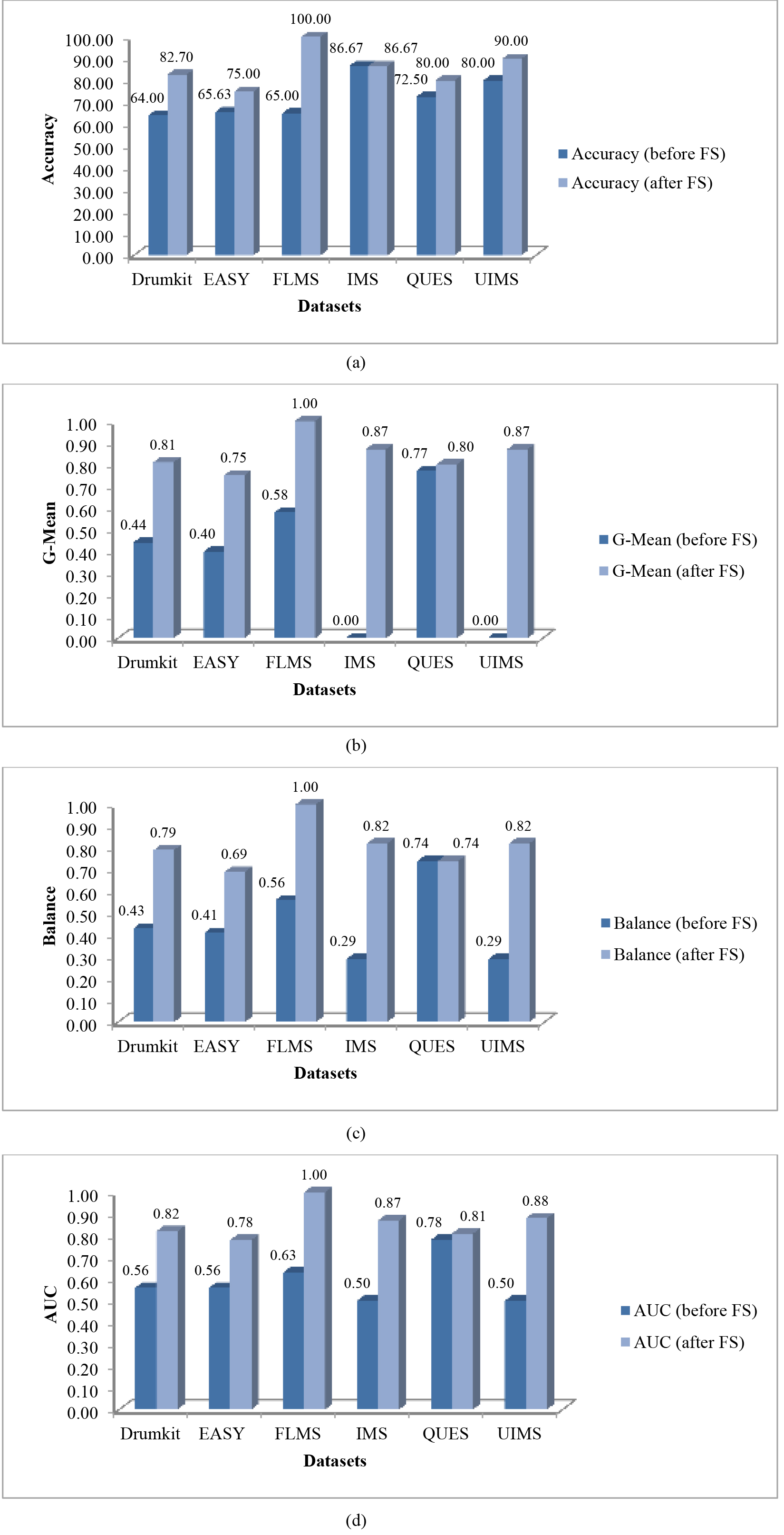

Further, on analyzing Tables 8–10, it has been observed that the values of G-Mean, Balance and AUC measures for all the datasets improved on applying various FS techniques for most of the cases as compared to the case where no FS has been used. Following this, Fig. 2a–d depict the median values obtained, before and after using FS techniques for each of the four accuracy measures, i.e., Accuracy, G-Mean, Balance, and AUC, respectively.

It is observed from Fig. 2a that the median values derived for Accuracy before using FS techniques are not so competitive. The highest median Accuracy value is attained by IMS dataset which is equal to 86.67%, whereas, this value is as low as 64% in case of Drumkit. Following this, from Fig. 2b it is clear that the median G-Mean values obtained for most of the datasets except QUES are extremely low without using FS. In fact, for IMS and UIMS datasets, this value is as low as 0.00, and the median G-Mean value for the FLMS dataset is close to 50%, i.e., 0.58. Likewise, as per Fig. 2c, the median Balance values obtained for almost all the datasets before using FS are also very low, except QUES having a median Balance value equal to 0.74.

On the other hand, IMS and UIMS datasets have the lowest median values for Balance equal to 0.29. Further, Fig. 2d again indicates lower median AUC values without using FS techniques for most of the datasets, except QUES and FLMS. However, the median AUC values for IMS and UIMS datasets are precisely equal to 0.50. This poor performance may be attributed to the presence of the redundant, irrelevant and noisy data, which degrades the learning of the prediction model being developed. That is why different FS techniques have been used in this study for removing insignificant features from the datasets and to investigate their effect in improving the performance of various prediction models so developed.

The median values of Accuracy, G-Mean, Balance, and AUC in Fig. 2 (after using FS) when compared with the corresponding values in Fig. 2 (before using FS) show that the use of various FS techniques indeed brought about a remarkable improvement in the performance of the different predictive models for all the datasets. Precisely, on the basis of median Accuracy values in Fig. 2a (before and after using FS techniques), an improvement of 29.22%, 14.28%, 53.85%, 10.34%, and 12.50% has been attained for Drumkit, EASY, FLMS, QUES, and UIMS datasets respectively by using FS; whereas in this case, no improvement has been observed for IMS dataset. In terms of median G-Mean values provided in Fig. 2b, the use of FS techniques resulted in an improvement equal to 84.09% for the Drumkit dataset, 87.50% for the EASY dataset, 72.41% for FLMS dataset, 87.00% for both IMS and UIMS datasets, and 3.90% for QUES dataset. Further, based on the median Balance values given in Fig. 2c, an improvement equal to 83.72% for Drumkit dataset, 68.29% for the EASY dataset, 78.57% for FLMS dataset, and 182.76% for IMS and UIMS datasets has been achieved after FS with no improvement in case of QUES dataset as the median Balance values for QUES are same in both the cases, i.e., before and after applying FS. Lastly, as shown in Fig. 2 (d), an improvement of 46.43%, 39.29%, 58.73%, 74.00%, 3.85%, and 76.00% has been observed for Drumkit, EASY, FLMS, IMS, QUES, and UIMS datasets respectively concerning the median AUC values on applying various FS techniques.

On an average, an overall improvement equal to 18.58%, 129.73%, 80.00%, and 45.76% in the median values of Accuracy, G-Mean, Balance, and AUC respectively has been attained on employing FS techniques for all the datasets taken together. Therefore, by virtue of the above results, it is concluded that the performance of different ML algorithms used in this study improves markedly by utilizing various FS techniques to predict software maintainability. Hence, this answers the first RQ (RQ1) raised in the current study.

5.3 Results of the Friedman test using different FS techniques

This sub-section attempts to answer RQ2 for carrying out a comparison between different FS techniques. RQ2 has been stated as RQ2: Which FS technique performs the best amongst the different FS techniques evaluated in this study?

As already concluded in Section 5.2, the use of FS techniques notably improved the performance of various predictive models developed using different ML techniques for all the six datasets with reference to Accuracy, G-Mean, Balance and AUC. However, the question that still remains unanswered is which of the three FS techniques used in the current work comparatively performed better. So, to carry this work further, the statistical Friedman test has been performed to answer the above question. This test has been applied for comparing four FS techniques in all, including SU, RFI, and CFS techniques, along with the scenario when no FS has been done. Therefore, the degree of freedom here is ‘ $r-1$ ’, i.e., $4-1=3$ and the level of significance, i.e., $\alpha$ is equal to 0.05. Friedman test has been applied by evaluating the values for each of the four performance measures, viz., Accuracy, G-Mean, Balance and AUC employing all the four cases of FS techniques for all the datasets.

5.3.1 Results of the Friedman test using different FS techniques with reference to Accuracy

The hypothesis of the Friedman test with reference to Accuracy measure has been stated as follows:

Null Hypothesis ( $H_{01}$ ): Various SMP models that have been built using different ML techniques (SVM, RF, DT (rpart), $k$ NN, Bagged CART, GPRR, C4.5-like Trees, & CIRF) do not exhibit notable differences in the performance when different FS techniques (SU, RFI, & CFS) are used as compared to the case when no FS is done with reference to Accuracy.

Alternate Hypothesis ( $H_{A1}$ ): Various SMP models that have been built using different ML techniques (SVM, RF, DT (rpart), $k$ NN, Bagged CART, GPRR, C4.5-like Trees, & CIRF) exhibit notable differences in the performance when different FS techniques (SU, RFI, & CFS) are used as compared to the case when no FS is done with reference to Accuracy.

Table 11 depicts the Friedman test results in respect of Accuracy, showing the mean ranks assigned to all the three FS techniques, including no FS case for each of the six datasets with corresponding $p$ -values. It is observable from Table 11 that the SU FS technique has secured the best rank for five out of the six datasets; whereas, CFS technique in this case has obtained the worst rank for four out of the total datasets. This further indicates that in terms of Accuracy, a few datasets have provided better results when no FS has been performed. Furthermore, the $p$ -values in Table 11 indicate that Friedman test results are notable for four out of the six datasets, i.e., except IMS and UIMS with $p$ -values less than 0.05. This directs the conclusion towards the scenario where null hypothesis has been rejected and alternate hypothesis has been accepted stating that various FS techniques perform notably different from each other in respect of Accuracy. Resultantly, the supreme performance of SU technique in majority datasets has made this technique stood out from the rest.

Table 11
Results of the Friedman test using Accuracy measure

Datasets	Rank 1	Rank 2	Rank 3	Rank 4	$p$ -value
Drumkit	SU	RFI	CFS	No FS	0.002
	(1.63)	(1.81)	(2.81)	(3.75)
EASY	SU	RFI	No FS	CFS	0.001
	(1.56)	(1.81)	(3.13)	(3.50)
FLMS	SU	RFI	CFS	No FS	0.000
	(1.50)	(1.50)	(3.25)	(3.75)
IMS	No FS	SU	RFI	CFS	0.429
	(2.19)	(2.38)	(2.44)	(3.00)
QUES	SU	RFI	No FS	CFS	0.002
	(1.38)	(2.19)	(2.75)	(3.69)
UIMS	SU	RFI	No FS	CFS	0.011
	(1.69)	(1.88)	(3.13)	(3.31)

Table 12

Results of the Friedman test using G-Mean measure

Datasets	Rank 1	Rank 2	Rank 3	Rank 4	$p$ -value
Drumkit	SU	RFI	CFS	No FS	0.002
	(1.63)	(1.81)	(2.81)	(3.75)
EASY	SU	RFI	CFS	No FS	0.000
	(1.50)	(1.63)	(3.13)	(3.75)
FLMS	SU	RFI	CFS	No FS	0.000
	(1.50)	(1.50)	(3.25)	(3.75)
IMS	SU	RFI	CFS	No FS	0.000
	(1.81)	(1.81)	(2.38)	(4.00)
QUES	SU	RFI	No FS	CFS	0.008
	(1.50)	(2.25)	(2.63)	(3.63)
UIMS	SU	RFI	CFS	No FS	0.000
	(1.63)	(1.75)	(2.63)	(4.00)

5.3.2 Results of the Friedman test using different FS techniques with reference to G-Mean

The hypothesis of the Friedman test with reference to G-Mean measure has been stated as follows:

Null Hypothesis ( $H_{02}$ ): Various SMP models that have been built using different ML techniques (SVM, RF, DT (rpart), $k$ NN, Bagged CART, GPRR, C4.5-like Trees, & CIRF) do not exhibit notable differences in the performance when different FS techniques (SU, RFI, & CFS) are used as compared to the case when no FS is done with reference to G-Mean.

Alternate Hypothesis ( $H_{A2}$ ): Various SMP models that have been built using different ML techniques (SVM, RF, DT (rpart), $k$ NN, Bagged CART, GPRR, C4.5-like Trees, & CIRF) exhibit notable differences in the performance when different FS techniques (SU, RFI, & CFS) are used as compared to the case when no FS is done with reference to G-Mean.

Table 12 presents the results of the Friedman test in respect of the G-Mean measure for all the six datasets with mean ranks assigned to each of the three FS techniques along with the case when no FS has been done, and the corresponding $p$ -values. It is evident from Table 12 that the SU FS technique has obtained the best rank amongst all other FS techniques, including no FS for each of the six datasets. On the other hand, the worst rank has been obtained by the scenario when no FS technique has been used for five out of the six datasets, i.e., except QUES. Further, it has also been observed from the $p$ -values so obtained that the results of the Friedman test are noteworthy for five datasets out of a total of six having $p$ -values $<$ 0.005 ( $\alpha$ ). Subsequently, the supremacy of the SU FS technique in outperforming all the other FS techniques for all the six datasets leads to rejecting the null hypothesis and thereby accepting the alternate hypothesis, which states that different FS techniques show remarkable differences in their performances with regard to the values of G-Mean.

5.3.3 Results of the Friedman test using different FS techniques with reference to Balance

The hypothesis of the Friedman test with respect to Balance measure has been stated as follows:

Null Hypothesis ( $H_{03}$ ): Various SMP models that have been built using different ML techniques (SVM, RF, DT (rpart), $k$ NN, Bagged CART, GPRR, C4.5-like Trees, & CIRF) do not exhibit notable differences in the performance when different FS techniques (SU, RFI, & CFS) are used as compared to the case when no FS is done with reference to Balance.

Alternate Hypothesis ( $H_{A3}$ ): Various SMP models that have been built using different ML techniques (SVM, RF, DT (rpart), $k$ NN, Bagged CART, GPRR, C4.5-like Trees, & CIRF) exhibit notable differences in the performance when different FS techniques (SU, RFI, & CFS) are used as compared to the case when no FS is done with reference to Balance.

Table 13 presents the Friedman statistics, including the mean ranks assigned to each of the three FS techniques plus the case when no FS has been done and the corresponding $p$ -values for all the six datasets with respect to Balance measure. It is noticeable from Table 13 that the best rank has been obtained by the SU FS technique for five out of the six datasets. It is also evident from the $p$ -values so obtained that the Friedman statistics are significant for all the six datasets having $p$ -values less than or equal to 0.005. These $p$ -values, in turn, lead to the acceptance of the alternate hypothesis stating that the performance of the predictive models on using different FS techniques differs remarkably from each other when compared on the basis of the Balance measure. Here also, the SU technique of FS stood on top of the other techniques. However, the case when no FS has been performed achieved the worst rank for five of the six datasets, which further advocates for the usage of FS techniques in improving the performance of the models.

Table 13
Results of the Friedman test using Balance measure

Datasets	Rank 1	Rank 2	Rank 3	Rank 4	$p$ -value
Drumkit	SU	RFI	CFS	No FS	0.001
	(1.63)	(1.75)	(2.69)	(3.94)
EASY	SU	RFI	CFS	No FS	0.000
	(1.50)	(1.63)	(3.00)	(3.88)
FLMS	SU	RFI	CFS	No FS	0.000
	(1.50)	(1.50)	(3.25)	(3.75)
IMS	RFI	SU	CFS	No FS	0.000
	(1.69)	(1.81)	(2.50)	(4.00)
QUES	SU	RFI	No FS	CFS	0.005
	(1.44)	(2.25)	(2.69)	(3.63)
UIMS	SU	RFI	CFS	No FS	0.000
	(1.63)	(1.75)	(2.63)	(4.00)

5.3.4 Results of the Friedman test using different FS techniques with reference to AUC

The hypothesis of the Friedman test with respect to AUC measure has been stated as follows:

Null Hypothesis ( $H_{04}$ ): Various SMP models that have been built using different ML techniques (SVM, RF, DT (rpart), $k$ NN, Bagged CART, GPRR, C4.5-like Trees, & CIRF) do not exhibit notable differences in the performance when different FS techniques (SU, RFI, & CFS) are used as compared to the case when no FS is done with reference to AUC.

Alternate Hypothesis ( $H_{A4}$ ): Various SMP models that have been built using different ML techniques (SVM, RF, DT (rpart), $k$ NN, Bagged CART, GPRR, C4.5-like Trees, & CIRF) exhibit notable differences in the performance when different FS techniques (SU, RFI, & CFS) are used as compared to the case when no FS is done with reference to AUC.

Table 14 presents the results of the Friedman Test with regard to AUC measure. This table provides the mean ranks assigned to each of the three FS techniques along with the case when no FS has been done for all the six datasets and the corresponding $p$ -values. It is noteworthy that the SU FS technique has obtained the best rank amongst all the other FS techniques for each of the six datasets, whereas, on the other hand, worst rank has been obtained by the scenario when no FS technique has been used for five out of the six datasets. Further, it has also been observed that the results of the Friedman test are remarkable for each of the six datasets having $p$ -values less than 0.005 ( $\alpha$ ). This conclusion has driven towards the rejection of the null hypothesis and the acceptance of the alternate hypothesis, claiming that different FS techniques show notable differences in their performance with respect to the AUC values.

Table 14
Results of the Friedman test using AUC measure

Datasets	Rank 1	Rank 2	Rank 3	Rank 4	$p$ -value
Drumkit	SU	RFI	CFS	No FS	0.000
	(1.63)	(1.63)	(2.88)	(3.88)
EASY	SU	RFI	CFS	No FS	0.000
	(1.50)	(1.63)	(3.13)	(3.75)
FLMS	SU	RFI	CFS	No FS	0.000
	(1.50)	(1.50)	(3.25)	(3.75)
IMS	SU	RFI	CFS	No FS	0.000
	(1.81)	(1.94)	(2.25)	(4.00)
QUES	SU	RFI	No FS	CFS	0.003
	(1.50)	(2.13)	(2.63)	(3.75)
UIMS	SU	RFI	CFS	No FS	0.000
	(1.63)	(1.75)	(2.63)	(4.00)

Table 15

Results of the Wilcoxon Signed Ranks test using Accuracy measure (based on positive ranks)

Datasets	Drumkit	EASY	FLMS	IMS	QUES	UIMS
Pair of FS techniques
SU-CFS
Mean Rank	1.50	0.00	0.00	0.00	0.00	2.50
Asymp. Sig.	(0.034)	(0.016)	(0.010)	(0.102)	(0.011)	(0.026)
SU-RFI
Mean Rank	2.50	1.50	0.00	1.50	0.00	1.00
Asymp. Sig.	(0.270)	(0.221)	(1.000)	(1.000)	(0.068)	(0.655)

Overall, it is evident from Friedman test results that the SU FS technique has surpassed all the other FS techniques irrespective of the dataset and the performance measure being used. This exceptional performance of the SU technique may be attributed to the benefits which this technique provides. The values in SU technique are normalized in the range [0,1] and it compensates for the bias of mutual information towards the multi-valued features. As the name suggests, SU has symmetric nature and results in the reduced number of comparisons for a pair of features, say, ‘ $A$ ’ and ‘ $B$ ’ since $\textit{SU}(A,B)$ is equivalent to $\textit{SU}(B,A)$ .

5.4 Results of the Wilcoxon Signed Ranks test using different FS techniques

As stated in the previous section, the results of the Friedman test have already proved that a noteworthy difference exists between the performance of different FS techniques with SU technique performing the best for various performance measures including Accuracy, G-Mean, Balance, and AUC for all the datasets. However, to know about the differences between various related pairs of different FS techniques, post-hoc analysis using the Wilcoxon Signed Ranks test with Bonferroni correction has been performed. The results of this test further answer the third RQ, i.e., RQ3: Does any significant difference exist between different pairs of FS techniques analyzed in this study?

The Wilcoxon test has been used to compare the SU FS technique that has been ranked to be the most accurate technique for all the datasets by the Friedman test with the other two FS techniques (RFI and CFS) at the level of significance, $\alpha=$ 0.05. Since Bonferroni adjustment is made if ‘ $s$ ’ Wilcoxon post-hoc tests are performed after the Friedman test (here, $s=$ 2), the value of $\alpha$ is adjusted to $\alpha/s$ . Therefore, the effective or the final value of $\alpha$ here is equal to 0.025 (0.05/2 $=$ 0.025). Tables 15–18 put forth the results of the Wilcoxon Signed Ranks test for all the six datasets using Accuracy, G-Mean, Balance, and AUC measures, respectively.

Table 16
Results of the Wilcoxon Signed Ranks test using G-Mean measure (based on positive ranks)

Datasets	Drumkit	EASY	FLMS	IMS	QUES	UIMS
Pair of FS techniques
SU-CFS
Mean Rank	1.50	0.00	0.00	0.00	0.00	3.00
Asymp. Sig.	(0.034)	(0.018)	(0.010)	(0.102)	(0.012)	(0.033)
SU-RFI
Mean Rank	2.50	1.50	0.00	1.50	0.00	1.00
Asymp. Sig.	(0.270)	(0.225)	(1.000)	(1.000)	(0.068)	(0.655)

Table 17

Results of the Wilcoxon Signed Ranks test using Balance measure (based on positive ranks)

Datasets	Drumkit	EASY	FLMS	IMS	QUES	UIMS
Pair of FS techniques
SU-CFS
Mean Rank	1.50	0.00	0.00	0.00	0.00	4.00
Asymp. Sig.	(0.034)	(0.018)	(0.010)	(0.066)	(0.012)	(0.047)
SU-RFI
Mean Rank	2.00	2.50	0.00	2.25	0.00	1.00
Asymp. Sig.	(0.176)	(0.500)	(1.000)	(0.414)	(0.068)	(0.655)

Table 18

Results of the Wilcoxon Signed Ranks test using AUC measure (based on positive ranks)

Datasets	Drumkit	EASY	FLMS	IMS	QUES	UIMS
Pair of FS techniques
SU-CFS
Mean Rank	2.00	0.00	0.00	1.00	0.00	3.50
Asymp. Sig.	(0.043)	(0.018)	(0.010)	(0.141)	(0.012)	(0.040)
SU-RFI
Mean Rank	3.00	1.50	0.00	2.50	0.00	1.00
Asymp. Sig.	(0.396)	(0.225)	(1.000)	(0.785)	(0.068)	(0.655)

Though it is known from the results of the Friedman test that the SU FS technique has been ranked the best for all the six datasets; from Tables 15–18 it is evident that SU technique is not significantly different from the RFI technique at $\alpha=$ 0.025 for any of the six datasets and the four accuracy measures by virtue of the results of the Wilcoxon test. However, the SU technique is significantly superior to the CFS technique in the case of EASY, FLMS, and QUES datasets having $p$ -values less than 0.025 for all the four measures of performance, viz., Accuracy, G-Mean, Balance, and AUC.

6. Threats to validity

This section elucidates various threats to validity that have been encountered while conducting the current study.

Construct validity pertains to the correct selection and measurement of both the independent and the dependent variables while developing various prediction models. However, all the OO metrics used as the variables in this study have been selected from the most popular metric suites available in the literature that have already been used in developing several maintainability prediction models. Even the dependent variable used here, i.e., maintainability, measured in respect of the number of changes in the code lines, has also been used previously in several literature studies. The selection of OO metrics in this manner minimizes the construct validity threat for the variables. Further, the threat to construct validity can also arise while making a selection of various ML techniques for building the models, but an attempt has been made to reduce this threat to the minimum by selecting several ML techniques.

Internal validity is related to the effect that the independent variables put on the dependent variable, also known as the ‘causal effect.’ In this study, due to the imbalance existent in the classes of the original datasets, an attempt was made to handle these imbalanced datasets using a re-sampling technique. However, this brought about a change in the ratio of the data points of the minority and the majority classes, which might alter the initial causal effect and possibly let the threat to internal validity peep in. However, the performance of the predictive models being developed has been estimated using one traditional measure, i.e., Accuracy and the three most stable and robust accuracy measures; namely, G-Mean, Balance, and AUC, to minimize this threat.

Conclusion validity is associated with particular possibilities that may hinder the correct and precise analysis of the results from reaching a conclusion. Utmost care has been taken to avoid this threat by taking various steps. 10-fold cross-validation has been used while training the models to reduce any bias in the validation. Cross-validation also helped in mitigating any potential threat due to small size of the datasets. Further, multiple robust accuracy measures have been used for evaluating the performance. Lastly, two non-parametric tests, namely, the Friedman test and the Wilcoxon Signed Ranks test, have been performed for the statistical and post-hoc analysis of the predicted results to substantiate the conclusions further.

External validity is related to the expanse to which the results of a particular study could be generalized. In the current study, six different datasets from three different domains built under particular environments have been used for building the SMP models. Therefore, the results may generalize to other software built in similar environments whereas this may pose a threat while validating the results using software that has been developed under differing scenarios. Another threat to external validity could be the small size of the datasets used in the current study which might not be that relevant for today’s large software systems.

7. Conclusion and future direction

The current study initiated with the purpose of investigating the effect of various FS techniques in SMP since the early and timely prediction of classes with low maintainability can come as a boon to the software developers. This investigation is necessary to bring down the overall cost of development, especially the cost incurred in the maintenance phase in respect to time, money and even the human effort. To begin with, this study started with six different datasets, including one open source, three proprietaries, and two commercial datasets. Initially, these datasets were analyzed through their respective descriptive statistics and the Shapiro-Wilk test of normality. This was followed by the preprocessing step, which included the conversion of datasets into binary, removal of outliers, and handling of imbalanced datasets using the ImpS technique.

Further, the foremost step of this study, i.e., the selection of relevant features from all the datasets using various FS techniques (SU, RFI, and CFS), was carried out. FS was done to make the predictive task more efficient due to the elimination of redundant and noisy data. After this, the final preprocessed datasets were used to build different prediction models using eight different ML techniques with 10-fold cross-validation. The performance of these models was estimated using one traditional measure, namely, Accuracy and three other robust performance measures, namely, G-Mean, Balance and AUC, to study and analyze the effect of different FS techniques on the predictive ability of the SMP models. Lastly, a statistical and post-hoc analysis using the Friedman test and the Wilcoxon Signed Ranks test was also conducted to further support the conclusions of this study. The major conclusions drawn are stated as follows:

•

The performance of the SMP models that have been developed using various ML algorithms improved remarkably on using different FS techniques for all the six datasets.

•

Of all the three FS techniques used here, the SU technique performed the best in predicting maintainability with respect to all the four performance measures, viz., Accuracy, G-Mean, Balance and AUC. However, the other two FS techniques, i.e., RFI and CFS, also provided competitive results compared to the case when no FS was done.

•

On comparing the best FS technique, i.e., SU with the other two FS techniques, it was found that the SU technique is superior to the CFS technique with reference to the EASY, FLMS and QUES datasets in respect of all the four measures of performance as mentioned above.

Thus, the current study would help the research community determine the low maintainability classes well in advance by developing efficient prediction models using various FS techniques. This would lead to judicious use of the resources concerning the developer’s time, money and effort by removing the unnecessary data through FS. As a future extension, the authors plan to implement the current work on a wide range of datasets that have been built using different languages under varying environments. Furthermore, the authors plan to utilize, analyze, and compare several other re-sampling methods and FS techniques apart from those used in this study for efficient model development. Last but not least, the authors plan to replace the ML techniques with various evolutionary, meta-heuristic, or hybridized techniques.

Footnotes

Acknowledgments

This research work has been supported by the O/o Director (Research and Consultancy), GGSIPU under the FRGS scheme through the project entitled, “Determination of Optimum Refactoring Sequence after Prioritization of Classes on the basis of their bad smell,” dt. 03.05.2019, Ref. No. GGSIPU/DRC/FRGS/ 2019/1553/62.

References

Aggarwal

K.K.

Singh

Kaur

and Malhotra

, Application of artificial neural network for predicting maintainability using object-oriented metrics, Transactions on Engineering, Computing and Technology 2(10) (2008), 3552–3556. doi: 10.5281/zenodo.1058483.

Ahmed

M.A.

and Al-Jamimi

H.A.

, Machine learning approaches for predicting software maintainability: a fuzzy-based transparent model, IET software 7(6) (2013), 317–326. doi: 10.1049/iet-sen.2013.0046.

Alsolai

Roper

and Nassar

, Predicting software maintainability in object-oriented systems using ensemble techniques. In: IEEE International Conference on Software Maintenance and Evolution (ICSME), IEEE, September 23–29, 2018, pp. 716–721. doi: 10.1109/ICSME.2018.00088.

Alsolai

and Roper

, Application of ensemble techniques in predicting object-oriented software maintainability. In: Proceedings of the Evaluation and Assessment on Software Engineering, ACM, April 15–17, 2019, pp. 370–373. doi: 10.1145/3319008.3319716.

Arisholm

Briand

L.C.

and Johannessen

E.B.

, A systematic and comprehensive investigation of methods to build and evaluate fault prediction models, Journal of Systems and Software 83(1) (2010), 2–17. doi: 10.1016/j.jss.2009.06.055.

Baskar

and Chandrasekar

, An Evolving Neuro-PSO-based Software Maintainability Prediction, International Journal of Computer Applications 179(18) (2018), 7–14. doi: 10.5120/ijca2018916305.

Bhatia

Chug

and Singh

A.P.

, Application of extreme learning machine in plant disease prediction for highly imbalanced dataset, Journal of Statistics and Management Systems 23(6) (2020), 1059–1068. doi: 10.1080/09720510..

Breiman

, Bagging predictors, Machine Learning 24(2) (1996), 123–140. doi: 10.1007/BF00058655.

Breiman

, Random forests, Machine Learning 45(1) (2001), 5–32. doi: 10.1023/A:1010933404324.

10.

Brezočnik

Fister

and Podgorelec

, Swarm intelligence algorithms for feature selection: a review, Applied Sciences 8(9) (2018), 1521. doi: 10.3390/app8091521.

11.

Carvalho

A.B.D.

Pozo

and Vergilio

S.R.

, A symbolic fault-prediction model based on multiobjective particle swarm optimization, Journal of Systems and Software 83(5) (2010), 868–882. doi: 10.1016/j.jss.2009.12.023.

12.

Chandrashekar

and Sahin

, A survey on feature selection methods, Computers & Electrical Engineering 40(1) (2014), 16–28. doi: 10.1016/j.compeleceng.2013.11.024.

13.

Chen

Menzies

Port

and Boehm

, Finding the right data for software cost modeling, IEEE software 22(6) (2005), 38–46. doi: 10.1109/MS.2005.151.

14.

Cherkassky

and Mulier

, Vapnik-Chervonenkis (VC) learning theory and its applications, IEEE Transactions on Neural Networks 10(5) (1999), 985–987. doi: 10.1109/TNN.1999.788639.

15.

Chidamber

S.R.

and Kemerer

C.F.

, A metrics suite for object oriented design, IEEE Transactions on software engineering 20(6) (1994), 476–493. doi: 10.1109/32.295895.

16.

Chug

and Malhotra

, Benchmarking framework for maintainability prediction of open source software using object oriented metrics, International Journal of Innovative Computing, Information and Control 12(2) (2016), 615–634.

17.

Cover

and Hart

, Nearest neighbor pattern classification, IEEE transactions on information theory 13(1) (1967), 21–27. doi: 10.1109/TIT.1967.1053964.

18.

Dagpinar

and Jahnke

J.H.

, Predicting maintainability with object-oriented metrics-an empirical comparison. In: 10th Working Conference on Reverse Engineering, 2003. WCRE 2003. Proceedings, IEEE, November 13–16, 2003, pp. 155–164. doi: 10.1109/WCRE.2003.1287246.

19.

Crawford

S.L.

, Extensions to the CART algorithm, International Journal of Man-Machine Studies 31(2) (1989), 197–217. doi: 10.1016/0020-7373(89)90027-8.

20.

Dallal

J.A.

, Object-oriented class maintainability prediction using internal quality attributes, Information and Software Technology 55(11) (2013), 2028–2048. doi: 10.1016/j.infsof.2013.07.005.

21.

Das

, Filters, wrappers and a boosting-based hybrid for feature selection, In: Proceedings of the Eighteenth International Conference on Machine Learning (ICML 2001), June 28–July 1, 2001, Vol. 1, pp. 74–81.

22.

Dash

and Liu

, Feature selection for classification, Intelligent Data Analysis 1(3) (1997), 131–156. doi: 10.1016/S1088-467X(97)00008-5.

23.

Datyal

Kaushik

and Tomar

, A Novel PCA based Multi-layer perceptron algorithm for Maintainability Prediction, International Journal of Engineering Trends and Technology 37(2) (2016), 90–96. doi: 10.14445/22315381/IJETT-V37P215.

24.

Dubey

S.K.

Rana

and Dash

, Maintainability prediction of object-oriented software system by multilayer perceptron model, ACM SIGSOFT Software Engineering Notes 37(5) (2012), 1–4. doi: 10.1145/2347696.2347703.

25.

Elish

M.O.

Aljamaan

and Ahmad

, Three empirical studies on predicting software maintainability using ensemble methods, Soft Computing 19(9) (2015), 2511–2524. doi: 10.1007/s00500-014-1576-2.

26.

Elish

M.O.

and Elish

K.O.

, Application of treenet in predicting object-oriented software maintainability: A comparative study, In: 13th European Conference on Software Maintenance and Reengineering, IEEE, March 24–27, 2009, pp. 69–78. doi: 10.1109/CSMR.2009.57.

27.

Gao

Khoshgoftaar

T.M.

and Napolitano

, Combining Feature Subset Selection and Data Sampling for Coping with Highly Imbalanced Software Data, In: The 27th International Conference on Software Engineering and Knowledge Engineering (SEKE), July 2015, pp. 439–444. doi: 10.18293/SEKE2015-182.

28.

Gunnalan

Menzies

Appukutty

Srinivasan

and Hu

, Feature subset selection with tar2less, 2003.

29.

Gupta

and Chug

, Assessing Cross-Project Technique for Software Maintainability Prediction, Procedia Computer Science 167 (2020), 656–665. doi: 10.1016/j.procs.2020.03.332.

30.

Gupta

and Chug

, Software maintainability prediction of open source datasets using least squares support vector machines, Journal of Statistics and Management Systems 23(6) (2020), 1011–1021. doi: 10.1080/09720510.2020.1799501.

31.

Gupta

and Chug

, Software maintainability prediction using an enhanced random forest algorithm, Journal of Discrete Mathematical Sciences and Cryptography 23(2) (2020), 441–449. doi: 10.1080/09720529.2020.1728898.

32.

Haixiang

Yijing

Shang

Mingyun

Yuanyue

and Bing

, Learning from class-imbalanced data: Review of methods and applications, Expert Systems with Applications 73 (2017), 220–239. doi: 10.1016/j.eswa.2016.12.035.

33.

Hall

M.A.

, Correlation-based feature selection for machine learning, The University of Waikato, 1999.

34.

Hall

M.A.

and Holmes

, Benchmarking attribute selection techniques for discrete class data mining, IEEE Transactions on Knowledge and Data engineering 15(6) (2003), 1437–1447. doi: 10.1109/TKDE.2003.1245283.

35.

Hasan

M.A.M.

Nasser

Ahmad

and Molla

K.I.

, Feature selection for intrusion detection using random forest, Journal of information security 7(3) (2016), 129–140. doi: 10.4236/jis.2016.73009.

36.

and Garcia

E.A.

, Learning from imbalanced data, IEEE Transactions on knowledge and data engineering 21(9) (2009), 1263–1284. doi: 10.1109/TKDE.2008.239.

37.

Hothorn

Bühlmann

Dudoit

Molinaro

and Van Der Laan

M.J.

, Survival ensembles, Biostatistics 7(3) (2006), 355–373. doi: 10.1093/biostatistics/kxj011.

38.

Hothorn

Hornik

and Zeileis

, Unbiased recursive partitioning: A conditional inference framework, Journal of Computational and Graphical statistics 15(3) (2006), 651–674. doi: 10.1198/106186006X133933.

39.

Jain

and Zongker

, Feature selection: Evaluation, application, and small sample performance, IEEE transactions on pattern analysis and machine intelligence 19(2) (1997), 153–158. doi: 10.1109/34.574797.

40.

Janabi

K.B.A.

and Kadhim

, Data Reduction Techniques: A Comparative Study for Attribute Selection Methods, International Journal of Advanced Computer Science and Technology(IJACST) 8(1) (2018), 1–13.

41.

Jha

Kumar

Abdel-Basset

Priyadarshini

Sharma

Long

H.V.

and others, Deep learning approach for software maintainability metrics prediction, IEEE Access 7 (2019), 61840–61855. doi: 10.1109/ACCESS.2019.2913349.

42.

Jia

Yang

Park

D.H.

Tan

and Park

, Software Maintainability Prediction Model Based on Fuzzy Neural Network, Journal of Multiple-Valued Logic & Soft Computing 20(1-2) (2013), 39–53.

43.

Jiang

Ding

Wang

and Xie

, A hybrid feature selection algorithm: Combination of symmetrical uncertainty and genetic algorithms, In: The second international symposium on optimization and systems biology (OSB’08), ORSC and APORC, October 31â€“-November 3, 2008, pp. 152–157.

44.

Kannan

S.S.

and Ramaraj

, A novel hybrid feature selection via Symmetrical Uncertainty ranking based local memetic search algorithm, Knowledge-Based Systems 23(6) (2010), 580–585. doi: 10.1016/j.knosys.2010.03.016.

45.

Kaur

and Malhotra

, Soft computing approaches for prediction of software maintenance effort, International Journal of Computer Applications 1(16) (2010), 69–75. doi: 10.5120/339-515.

46.

Khalid

Khalil

and Nasreen

, A survey of feature selection and feature extraction techniques in machine learning, In: Science and Information Conference, IEEE, August 27–29, 2014, pp. 372–378. doi: 10.1109/SAI.2014.6918213.

47.

Kohavi

John

and others, Wrappers for feature subset selection, Artificial intelligence 97(1-2) (1997), 273–324. doi: 10.1016/S0004-3702(97)00043-X.

48.

Koten

C.V.

and Gray

A.R.

, An application of Bayesian network for predicting object-oriented software maintainability, Information and Software Technology 48(1) (2006), 59–67. doi: 10.1016/j.infsof.2005.03.002.

49.

Kubat

Matwin

and others, Addressing the curse of imbalanced training sets: one-sided selection, In: Proceedings of the 14th International Conference on Machine Learning (ICML), Citeseer, 1997, Vol. 97, pp. 179–186.

50.

Kumar

Naik

D.K.

and Rath

S.K.

, Validating the effectiveness of object-oriented metrics for predicting maintainability, Procedia Computer Science 57 (2015), 798–806. doi: 10.1016/j.procs.2015.07.479.

51.

Kumar

and Rath

S.K.

, Hybrid functional link artificial neural network approach for predicting maintainability of object-oriented software, Journal of Systems and Software 121 (2015), 170–190. doi: 10.1016/j.jss.2016.01.003.

52.

Kumar

and Rath

S.K.

, Software maintainability prediction using hybrid neural network and fuzzy logic approach with parallel computing concept, International Journal of System Assurance Engineering and Management 8(2) (2017), 1487–1502. doi: 10.1007/s13198-017-0618-4.

53.

Zhang

and Zhou

, Sample-based software defect prediction with active and semi-supervised learning, Automated Software Engineering 19(2) (2012), 201–230. doi: 10.1007/s10515-011-0092-1.

54.

and Henry

, Object-oriented metrics that predict maintainability, Journal of systems and software 23(2) (1993), 111–122. doi: 10.1016/0164-1212(93)90077-B.

55.

Liu

and Yu

, Toward integrating feature selection algorithms for classification and clustering, IEEE Transactions on knowledge and data engineering 17(4) (2005), 491–502. doi: 10.1109/TKDE.2005.66.

56.

Luque

Carrasco

Martín

and Heras

A.D.L.

, The impact of class imbalance in classification performance metrics based on the binary confusion matrix, Pattern Recognition 91 (2019), 216–231. doi: 10.1016/j.patcog.2019.02.023.

57.

MacKay

D.J.C.

, Introduction to Gaussian processes, NATO ASI Series F Computer and Systems Sciences 168 (1998), 133–166.

58.

Malhotra

, A systematic review of machine learning techniques for software fault prediction, Applied Soft Computing 17 (2015), 504–518. doi: 10.1016/j.asoc.2014.11.023.

59.

Malhotra

and Chug

, Application of evolutionary algorithms for software maintainability prediction using object-oriented metrics, In: Proceedings of the 8th International Conference on Bioinspired Information and Communications Technologies, ACM, December 1–3, 2014, pp. 348–351. doi: 10.4108/icst.bict.2014.258044.

60.

Malhotra

and Chug

, Application of group method of data handling model for software maintainability prediction using object oriented systems, International Journal of System Assurance Engineering and Management 5(2) (2014), 165–173. doi: 10.1007/s13198-014-0227-4.

61.

Malhotra

and Chug

, Software maintainability prediction using machine learning algorithms, Software Engineering: An International Journal (SEIJ) 2(2) (2012), 19–36.

62.

Morasca

, A probability-based approach for measuring external attributes of software artifacts, In: 3rd International Symposium on Empirical Software Engineering and Measurement, IEEE, October 15–16, 2009, pp. 44–55. doi: 10.1109/ESEM.2009.5316048.

63.

Olatunji

S.O.

and Ajasin

, Sensitivity-based linear learning method and extreme learning machines compared for software maintainability prediction of object-oriented software systems, ICTACT Journal On Soft Computing 3(3) (2013), 514–523. doi: 10.21917/ijsc.2013.0077.

64.

Pan

and Shen

, Robust prediction of B-factor profile from sequence using two-stage SVR based on random forest feature selection, Protein and peptide letters 16(12) (2009), 1447–1454. doi: 10.2174/092986609789839250.

65.

Piao

and Lee

J.Y.

, Symmetrical uncertainty-based feature subset generation and ensemble learning for electricity customer classification, Symmetry 11(4) (2019), 498. doi: 10.3390/sym11040498.

66.

Potharaju

S.P.

and Sreedevi

, A Novel M-Cluster of Feature Selection Approach Based on Symmetrical Uncertainty for Increasing Classification Accuracy of Medical Datasets, Journal of Engineering Science & Technology Review 10(6) (2017), 154–162. doi: 10.25103/JESTR.106.20.

67.

Rao

Shi

Rodrigue

A.K.

Feng

Xia

Elhoseny

Yuan

and Gu

, Feature selection based on artificial bee colony and gradient boosting decision tree, Applied Soft Computing 74 (2019), 634–642. doi: 10.1016/j.asoc.2018.10.036.

68.

RStudio Team and others, RStudio: integrated development for R, RStudio, Inc., Boston, MA 42 (2015), 14. https://rstudio.com/.

69.

Saeys

Abeel

and Van de Peer

, Robust feature selection using ensemble feature selection techniques, In: Joint European Conference on Machine Learning and Knowledge Discovery in Databases (ECML PKDD 2008), Springer, September 15–19, 2008, pp. 313–325. doi: 10.1007/978-3-540-87481-2_21.

70.

Quinlan

, C4. 5: programs for machine learning, Morgan Kaufmann, 2014. (ISBN 1-55860-238-0).

71.

Sayed

G.I.

Hassanien

A.E.

and Azar

A.T.

, Feature selection via a novel chaotic crow search algorithm, Neural computing and applications 31(1) (2019), 171–188. doi: 10.1007/s00521-017-2988-6.

72.

Shapiro

S.S.

and Wilk

M.B.

, An analysis of variance test for normality (complete samples), Biometrika 52(3/4) (1965), 591–611. doi: 10.2307/2333709.

73.

Shatnawi

, Improving software fault-prediction for imbalanced data, In: International Conference on Innovations in Information Technology (IIT), IEEE, March 18–20, 2012, pp. 54–59. doi: 10.1109/INNOVATIONS.2012.6207774.

74.

Solorio-Fernández

Carrasco-Ochoa

J.A.

and Martínez-Trinidad

, A review of unsupervised feature selection methods, Artificial Intelligence Review 53(2) (2020), 907–948. doi: 10.1007/s10462-019-09682-y.

75.

Sunitha

BalRaju

Sasikiran

and Ramana

E.V.

, Automatic outlier identification in data mining using IQR in real-time data, International Journal of Advanced Research in Computer and Communication Engineering 3(6) (2014), 7255–7257.

76.

Sylvester

E.V.A.

Bentzen

Bradbury

I.R.

Clément

Pearce

Horne

and Beiko

R.G.

, Applications of random forest feature selection for fine-scale genetic population assignment, Evolutionary applications 11(2) (2018), 153–165. doi: 10.1111/eva.12524.

77.

Therneau

T.M.

and Atkinson

E.J.

, An introduction to recursive partitioning using the RPART routines. 2018, Mayo Foundation, 2019.

78.

Quah

and Thwin

M.M.T.

, Application of neural networks for software quality prediction using object-oriented metrics, In: Proceedings of International Conference on Software Maintenance (ICSM 2003), IEEE, September 22–26, 2003, pp. 116–125. doi: 10.1109/ICSM.2003.1235412.

79.

Vishwakarma

V.P.

and Dalal

, A novel non-linear modifier for adaptive illumination normalization for robust face recognition, Multimedia Tools and Applications 79 (2020), 11503-â€“11529. doi: 10.1007/s11042-019-08537-6.

80.

Wang

Gegov

Farzad

Chen

and Hu

, Fuzzy network based framework for software maintainability prediction, International Journal of Uncertainty, Fuzziness and Knowledge-Based Systems 27(5) (2019), 841–862. doi: 10.1142/S0218488519500375.

81.

Xue

Zhang

Browne

and Yao

, A survey on evolutionary computation approaches to feature selection, IEEE Transactions on Evolutionary Computation 20(4) (2016), 606–626. doi: 10.1109/TEVC.2015.2504420.

82.

Zheng

Zhu

Wen

Zhu

and Gan

, Unsupervised feature selection by self-paced learning regularization, Pattern Recognition Letters 132 (2020), 4–11. doi: 10.1016/j.patrec.2018.06.029.

83.

Zhou

and Leung

, Predicting object-oriented software maintainability using multivariate adaptive regression splines, Journal of systems and software 80(8) (2007), 1349–1361. doi: 10.1016/j.jss.2006.10.049.

84.

Zimmerman

D.W.

and Zumbo

B.D.

, Relative power of the Wilcoxon test, the Friedman test, and repeated-measures ANOVA on ranks, The Journal of Experimental Education 62(1) (1993), 75–86. doi: 10.1080/00220973.1993.9943832.

85.

Romanski

Kotthoff

and Kotthoff

M.L.

, Selecting Attributes, Package â€˜FSelector’, pp. 1–18. https://cran.r-project.org/web/packages/FSelector/FSelector.pdf.

86.

SES Subcommittee, IEEE standard for software maintenance, IEEE Std, 1992, pp. 1219–1993. doi: 10.1109/IEEESTD.1993.115570.

87.

R Core Team and others, R: A language and environment for statistical computing, 2013. https://cran.r-project.org/bin/windows/base/old/4.0.0/.

88.

Paula

Rita

and Luis

, An Implementation of Re-Sampling Approaches to Utility-Based Learning for Both Classification and Regression Tasks, R Package ‘UBL’ (2017) 1 –61. https://cran.r-project.org/web/packages/UBL/UBL.pdf, https://github.com/paobranco/UBL.

Datasets	No. of data points	L-M	H-M	I-R	No. of outliers	No. of data points after outlier removal
Drumkit	91	30	61	2.03	8	83
EASY	58	21	37	1.76	6	52
FLMS	34	14	20	1.43	3	31
IMS	47	10	37	3.70	0	47
QUES	71	30	41	1.37	6	65
UIMS	39	09	30	3.33	6	33

A feature selection strategy for improving software maintainability prediction

Abstract

Keywords

1. Introduction

2.1 Background work related to SMP

2.2 Background work related to FS techniques

3. Research background

Table 1 Definition table for the OO metrics [54]

4.3 Handling the imbalanced datasets

4.4 Feature Selection (FS) techniques

4.4.1 Symmetrical Uncertainty (SU)

4.4.3 Correlation-based Feature Selection (CFS)

4.6 Performance evaluation measures

Table 5 Confusion matrix

Table 6 Table for Feature Selection (FS)

5.1 Feature Selection (FS) results

5.2 Evaluation and discussion of results using different FS techniques and ML algorithms with 10-fold cross-validation

5.3.1 Results of the Friedman test using different FS techniques with reference to Accuracy

Table 11 Results of the Friedman test using Accuracy measure

5.3.3 Results of the Friedman test using different FS techniques with reference to Balance

Table 13 Results of the Friedman test using Balance measure

Table 14 Results of the Friedman test using AUC measure

Table 16 Results of the Wilcoxon Signed Ranks test using G-Mean measure (based on positive ranks)

7. Conclusion and future direction

Footnotes

Acknowledgments

References

Table 1
Definition table for the OO metrics [54]

Table 5
Confusion matrix

Table 6
Table for Feature Selection (FS)

Table 11
Results of the Friedman test using Accuracy measure

Table 13
Results of the Friedman test using Balance measure

Table 14
Results of the Friedman test using AUC measure

Table 16
Results of the Wilcoxon Signed Ranks test using G-Mean measure (based on positive ranks)