An integrated model based on feedforward neural network and Taylor expansion for indicator correlation elimination

Abstract

Existing correlation processing strategies make up for the defect that most evaluation algorithms do not consider the independence between indicators. However, these solutions may change the indicator system’s internal connection, affecting the final evaluation result’s interpretability and accuracy. Besides, traditional independent analysis methods cannot accurately describe the complex multivariate correlation based on the linear relationship. Aimed at these problems, we propose an indicators correlation elimination algorithm based on the feedforward neural network and Taylor expansion (NNTE). Firstly, we propose a generalized n-power correlation and a feedforward neural network to express the relationship between indicators quantitatively. Secondly, the low-order Taylor expression expanded at every sample is pointed to eliminate nonlinear relationships. Finally, to control the expansions’ accuracy, the layer-by-layer stripping method is presented to reduce the dimensionality of the correlations among multiple indicators gradually. This procedure continues to iterate until there are all simple two-dimensional correlations, eliminating multiple variables’ correlations. To compare the elimination efficiency, the ranking accuracy is proposed to measure the distance of the resulting sequence to the benchmark sequence. Under Cleveland and KDD99 two datasets, the ranking accuracy of the NNTE method is 71.64% and 96.41%, respectively. Compared with other seven common elimination methods, our proposed method’s average increase is 13.67% and 25.13%, respectively.

Keywords

System evaluation indicator correlation neural network Taylor expansion dimension reduction

ï»¿

1. Introduction

The endogenous process in nature is often a time-sequential variation between multiple variables [9]. The univariate evaluation’s assumption is inconsistent with reality. We take an interest in the data vector group organized in time series to expand the application scope. When using multiple indicators to evaluate one target as a whole, it is inseparable from the evaluation algorithm’s support. This calculation procedure is a concrete realization of integrating multiple indicators under the evaluation theory’s guidance. In the evaluation, the order of the results is more important than the specific value. Therefore, the ranking accuracy is used to show the goodness of the evaluation result.

According to the number of indicators, method characteristics, and requirements, we classify the existing 16 classic evaluation methods in the evaluation field. In univariate evaluation methods, such as exponential evaluation method (EEM) [3], comparison matrix method (CMM) [55], and product comparison method (PCM) [33], each indicator can reflect the characteristics of a specific aspect of the selected target. However, we cannot obtain its overall evaluation. To solve this problem, many researchers have proposed the deterministic evaluation methods for multiple indicators, including the weighted sum method (WSM) [18], weighted product method (WPM) [42], analytic hierarchy process (AHP) [38], and entropy value method (EVM) [53]. In these methods, all data and information are assumed to be precise; it is challenging to analyze the phenomenon of uncertainty. Therefore, grey relational analysis (GRA) [41], the technique for order preference by similarity to an ideal solution (TOPSIS) [28], and rough evaluation method (REM) [51] are proposed to solve the quantitative problem of qualitative factors. Further, the evaluation method has been adaptively expanded. Deterministic evaluation methods are suitable for handling multiple sets of data (such as cluster analysis (CA) [6] and attack graph model (AGM) [44]). Uncertainty evaluation methods are based on subjective data input (such as fuzzy evaluation method (FEM) [13] and dynamic Bayesian method (DBM) [27]).

The above methods focus on a variety of problems encountered in the calculation process of comprehensive evaluation. Notably, these evaluation methods all assume that indicators are mutually independent [32, 8, 47]. However, they ignore the hidden correlations between the indicator variables. This neglected repeated calculation makes the rank of the evaluation results wrong. The specific examples of improper ranking results and their effects are as follows: (1) In the regional economic development plan [40], the fundamental indicators include economic efficiency indicators, environmental indicators, and foreign investment attraction indicators. They are not entirely mutually independent. For example, while the real estate industry’s economic benefits are usually higher than in other tertiary industries, its damage to the environment is more remarkable. These two factors show a reverse synergistic relationship. Suppose we use these redundant components for evaluation without correlation processing. Then promising projects’ funding may be lower than that of disadvantaged projects, which is not conducive to the local economy’s coordinated and sustainable development. (2) When the administrative institution allocates the police force, it would consider the unemployment rate, property status, and non-white ratio. The unemployment rate of non-whites is usually higher [12]. If there is no correlation treatment, many workforce and financial resources may be poured into places with low crime levels, resulting in a high overall crime rate. (3) There is a link between credit and consumption capacity. So when social assistance is issued, improper asset evaluation may help taxes flow into low-income people who have social security instead of the hungry homeless [19]. This social injustice undermines social stability and prosperity. Therefore, it has become an important research point to restore the correct ranking of evaluation results by reducing or eliminating the implicit correlation between indicator variables.

According to their processing stages, seven mainstream models of studying the correlation between indicators can be divided into two categories. One is to process at the beginning, including indicator number limitation (INL) [7, 25], overlapping factors separation (OFS) [35]; the other is to deal with indicators in the middle stage by means of mathematical transformation, including indicator weight revision (IWR) [52], independent component analysis (ICA) [37, 1], principal component analysis (PCA) [45, 43], logistic regression (LR) [10], and multilayer perceptrons (MLP) [15, 48].

The INL method is similar to the feature selection method [30] in the data preprocessing stage, and both achieve better and faster evaluation results by limiting the number of indicators. But the purpose of the two is different. The latter determines whether to retain the indicator by evaluating the degree of relevance to the target, while the former limits the number of indicators as much as possible to minimize the hidden overlap that may exist between indicators. This method is simple to operate, but the relevant parts and overlapping parts of each indicator are bound together, which may mistakenly eliminate its unique information. OFS solves this problem well. It eliminates relevant parts by measuring how much the overlapped part accounts for the amount of indicator information. However, this method is used to eliminate monotonic correlation, and cannot be used to solve non-monotonic correlation problems. IWR adjusted the modified part to the parameters. Its implementation usually appears together with algorithms such as WSM, and the approach is to use modified weights to offset overlapping calculations. However, this method is a compromise on the calculation method, and no mutually independent indicators have been obtained. PCA compresses a set of indicators with a certain relationship into a few comprehensive indicators through linear combination, called principal components. However, the existence of principal components often does not have practical significance, and it is usually used to satisfy the sample point set of Gaussian distribution, which reduces the versatility of the method. ICA is a generalization of PCA, which can be used to find non-Gaussian factors. Under the assumption that the factors exist, each common factor is given a practical meaning, and its essence is to fit the original variable with a linear combination of factors. However, due to the existence of factor rotation, the solution is not unique, and there is a loss of variance in the solution process, so it is difficult to retain all the useful information. LR uses the maximum likelihood idea, which is essentially a two-class model. It uses each index as the input to predict whether the classification of the target is accurate as a benchmark for judging the strength of the correlation. The structure is simple and the training speed is fast. However, due to the linear decision-making surface of logistic regression, it cannot effectively deal with nonlinear problems, and the low degree of fitting of the model results in its low accuracy rate. MLP can be understood as a simple neural network, and non-linear activation functions can help train non-linear sample sets. When there are more than two hidden layers, the model can better capture the characteristics of nonlinear correlation. But this method relies on the training of network parameters and the intermediate process is difficult to explain.

Specifically, different methods have different effects on the indicator system and the application area. For this reason, we analyzed the above models from different aspects, including the mathematics field to which it belongs, whether the indicator system or indicators’ meaning is modified, the appropriate fields, and the description of these methods. The final results are shown in Table 1.

Table 1
Classification of indicator correlation elimination

Model	Mathematics	Modification		Applicable scenarios	Method description
		SYS Sav	IND Sav
INL	Basic Math $+$ System Theory	$\times$	$\surd$	The indicator system is small and could be simplified	Fundamental, decrease in number, and incomplete
OFS	Matrix Theory	$\surd$	$\times$	Indicators are linearly independent and could be decomposed	Fundamental, decomposition of indicators, non-linear difficult
IWR	Matrix Theory	$\surd$	$\surd$	Indicators are linearly independent and weighable	Weight correction, nonlinear difficult
ICA	Applied Statistics	$\times$	$\times$	Hidden factors exist	Factorization, measurable nonlinearity
PCA	Applied Statistics	$\times$	$\times$	Principal components exist	Principal component extraction, measurable nonlinearity
LR	Statistics $+$ Probability Theory	$\surd$	$\surd$	Widely applicable, input and output related	Linear regression, nonlinearity easy to test
MLP	Statistics $+$ Probability Theory	$\surd$	$\surd$	Widely applicable, input and output related	Neural networks, nonlinearity easy to test

According to Table 1, ICA, PCA and INL change indicator system’s structure. Regarding the impact on the indicator system structure, the existential hypothesis of ICA’s hidden factors and the available premise of PCA’s principal components have changed the parallel relationship between the same level indicators and the hierarchical relationship between the upper and lower indicators. Furthermore, the number of factors and principal components appear as hyperparameters in the evaluation test, making the meaning of each element difficult to explain. INL is suitable for the evaluation scenario with a small number of indicators. However, when faced with a host of indicators, the comprehensiveness of synthesis evaluation and the indicator system’s simplicity form a dilemma. In this case, the correlation between indicators cannot be eliminated. The other four methods aim to eliminate the correlation of indicators while keeping the indicator system structure unchanged. Among them, OFS and IWR are based on the separation strategy to extract mutually independent parts from the indicators or weights. Nevertheless, the correlation degree calculation still relies on the traditional linear correlation method, failing to eliminate the deeper and complex variable correlation between indicators. LR and MLP find the functional relationship between different indicator variables from the original data based on machine learning. Similarly, the above two methods still do not describe the complex correlation between indicator variables. Moreover, poor training models and parameter settings tend to treat measurement errors as irrelevant parts, making the elimination invalid.

To sum up, the current indicator correlation elimination algorithm does not consider the indicator system’s consistency and the nonlinear correlation between indicator variables. Hence, it is arduous to explain the indicator system’s meaning and achieve the evaluation indicator’s complete independence. To improve the evaluation’s accuracy, researchers must propose new definitions and strategies to characterize these intricate relationships between indicators. Simultaneously, different response methods need to be given to every sample point to minimize the measurement errors that interfere with the evaluation results. To achieve these above goals, this paper defines generalized n-power correlation, extending the linear correlation to the general correlation. Furthermore, combining MLP and OFS, a method based on the feedforward neural network and low-order Taylor expansion (NNTE) to eliminate the correlation of evaluation indicators is proposed. In particular, the relationship between the multi-dimensional indicators is gradually reduced to the calculation of the relationship between two indicators using the layer-by-layer stripping method.

The rest of this paper is organized as follows. Section 2 introduces the background knowledge and research status of indicator correlation elimination. In Section 3, we introduce the method of eliminating the nonlinear correlation between multiple indicators based on NNTE. Section 4 analyzes the experimental datasets and compares the effectiveness of the correlation elimination strategy proposed in this paper with other mainstream evaluation algorithms. We summarize this paper’s research in Section 5. Section 6 puts forward the shortcomings and possible future research directions.

2. Related work

The traditional correlation elimination method can trace back to the famous Pearson correlation coefficient [39] proposed by the British statistician Karl Pearson in the 1890s. He advocated calculating the linear correlation between two indicators by the ratio of the covariance and the product of variance. Specifically, OFS and IWR usually use this coefficient to calculate the overlap’s size. Mainstream correlation elimination methods also include the Spearman coefficient [20], Kendall coefficient [23], and their variants.

It is worth noting that in the Pearson coefficient, the two variance values at the denominator position cannot be zero. In other words, neither of the two variables can be constants, which limits the scope of application. In addition, this coefficient does not restrict outliers, which makes the evaluation results sensitive to noise interference. To solve these two problems, the Spearman coefficient introduces the concept of rank. This parameter indicates the ranking position of each sample point in the sample set, regardless of the specific value, thereby reducing the dependence on the size of individual variables. To deal with the problem that the Pearson coefficient cannot solve the correlation measurement of categorical variables, the Kendall coefficient puts forward the concept of ordered pairs. It uses the consistency of the ordering relationship between two adjacent ordered pairs as a benchmark and calculates the ratio of the difference between the identical ordered pairs and the inconsistent ordered pairs to the total number of sequences. Although the Spearman coefficient and Kendall coefficient extend the measurable linear correlation of the Pearson coefficient to monotonic correlation, they still cannot effectively deal with the measurement of complex functional correlations such as square relationship, logarithmic relationship, exponential relationship, and triangular periodic function. Therefore, when using multiple indicators to evaluate, a similar linear or monotonic processing method for all variables without judgment may change the final evaluation results’ comparison order. Therefore, this disorder increases the false-negative rate (judging serious incidents as normal behaviors) and the false-positive rate (judging non-serious objects as urgent incidents). This misjudgment puts forward higher requirements for studying the fuzzy relationship between deeper bottom evaluation indicators.

To extend the correlation elimination to the non-linear and monotonic field, many scholars have made a lot of related research. Among them, the classic method is based on mutual information [17]. Mutual information takes the probability density function of the bivariate as the known relationship, so it can measure complex correlation relationships including non-linear relationships. The correlation elimination method based on mutual information is usually used to solve the correlation relationship of bivariate continuous functions. For sample sets composed of multivariate discrete points such as network security datasets and medical datasets, the solution of the probability function is an NP-hard problem.

In recent years, to make the evaluation results more credible and reliable, many researchers have done a lot of related work in proposing global indicator processing methods. Paper [9] proposed a method called independent component analysis (ICA), suitable for multivariate data. It estimates independent components by combining non-parametric probability integral transformation with generalized non-parametric whitening methods. Paper [56] proposed three new methods to measure the interdependence between multiple random variables. The first method generalizes the distance covariance from pairwise dependence to mutual dependence. The other two methods are the sum of distance covariance squares. Both two methods are used to capture the nonlinear and non-monotonic interdependence between random vectors. Based on the mean-variance indicator, Paper [16] proposed an unconditional distribution function for continuous variables under a given discrete value. This function is aimed at testing the correlation between discrete variables and continuous variables. Paper [4] proposed two new feature-weighted L2 distance measurement methods based on random variables: distance multivariate and total distance multivariate. They can deal with the correlation between multiple random variables and extend the distance covariance from paired random variables to n-ary random variables. Paper [57] proposed a probabilistic model based on the multivariate Polya tree. It can test the mutual independence between continuous random variable vector groups. Moreover, the obtained Bayes factor is used for the independence test.

3. Methodology

Since the assumption of linear correlation does not match the actual situation, we introduce the concept of the multi-dimensional correlation between variables. To express this concept quantitatively, we adjust the existing neural network structure to find the relationship between input and output indicators. OFS and IWR make the same adjustments to weights or values at all sample points. However, this operation affects the accuracy of expression expansion. Consequently, we adopt different adjustment strategies at different sample points. Meanwhile, to extend the relationship between two variables to multiple variables, we adopt the idea of peeling off the relevant parts layer-by-layer to reduce dimensionality.

3.1 N-power correlation

The Pearson coefficient, which is widely used in the industry to measure the correlation between indicators, is defined as:

$\displaystyle\rho_{xy}=\frac{\text{cov}(x,y)}{\sqrt{\text{var}(x)}\sqrt{\text{% var}(y)}}$ (1)

where $\text{cov}({x},{y})$ denotes the covariance between the variables $x$ and $y$ , $\text{var}({x})$ and $\text{var}({y})$ denote the variance of the variable $x$ and $y$ respectively.

However, Eq. (1) can only measure the cooperative change relationship between two variables. What is more, it is essentially a linear transformation based on the calculation of the mean value, which does not apply to significant nonlinear relationships. For example, in the bivariate relationship $y={x}^{2}$ , $x\sim{N}(0,1)$ , it can be seen that the relationship between ${x}$ and ${y}$ is intensely close, showing a functional relationship. However, when using Pearson’s coefficient to measure the correlation in this function:

$\displaystyle\text{cov}(x,y)=E(x-E(x))(y-E(y))=E(x^{3})-E(x)E(x^{2})=0$ (2)

It is manifest from Eq. (2) that although the Pearson coefficient is zero, there is still a notable functional correlation between ${x}$ and ${y}$ . Starting from a set of sample points $(({x}{}_{1},{y}_{1}),({x}_{2},{y}_{2}),\ldots,({x}_{m},{y}_{m}))$ , for a large number of sample points, the Pearson correlation can always be calculated. However, this coefficient can only reflect the degree of linear correlation, not the degree of correlation of complex functional relationships.

This paper defines square correlation, cubic correlation, and n-power correlation, extending linear correlation to high-dimensional correlation to describe complex function relationships.

Let ${Y}=\{{y}_{i}:i=1,\ldots,m\}$ be the independent and identically distributed sample points of the joint distribution function of the random vector $(x_{1},x_{2},\cdots,x_{n})\to y_{i}\in{\rm{\rm R}}^{m}$ .

Definition 1. Square correlation. When the dependent variable ${y}$ satisfies ${y}\sim ax^{2}$ , the correlation between ${x}$ and ${y}$ is called square correlation. The closer to ${ax}^{2}$ , the greater the square correlation. Its value range is [0, 1];

Definition 2. Cube correlation. when the dependent variable ${y}$ satisfies ${y}\sim{ax}^{3}$ , the correlation between ${x}$ and ${y}$ is called cube correlation. The closer to ${ax}^{3}$ , the greater the cube correlation. Its value range is [0, 1];

Definition 3. N-power correlation. when the dependent variable ${y}$ satisfies ${y}\sim ax^{n}$ , the correlation between ${x}$ and ${y}$ is called n-power correlation. The closer to ${ax}^{n}$ , the greater the n-power correlation. Its value range is [0, 1].

3.2 Taylor expansion

The Taylor expansion contains the order relationship between the input and output variables. The stronger a certain relationship is, the larger the constant coefficient in front of its expansion. This characteristic is consistent with the characteristic of the n-power correlation depicted in Section 3.1. The Taylor formula also supports expanding at discrete points. Therefore, to measure the correlation at different points, this paper expends the Taylor formula to a certain order.

We assume that the random vector variable ${y}$ has a non-singular continuous distribution function $f_{x\to y}$ , and satisfies $E(y)>0$ and $E|y|^{2}<\infty$ .

If the unary function $f:x\to y$ is $n+1$ th order derivable at the point ${x}_{0}$ and $n$ is a positive integer, then the following formula is satisfied:

$\displaystyle f(x)=\sum\limits_{n=0}^{N}\frac{f^{(n)}(x_{0})}{n!}(x-x_{0})^{n}% +R_{n}(x)$ (3)

If the binary function $f:({x}_{1},{x}_{2})\to{y}$ is $n+1$ th order derivable at the point $x^{(0)}=(x_{1}^{(0)},x_{2}^{(0)})$ , then the following formula is satisfied:

$\displaystyle f(x_{1},x_{2})=\sum\limits_{j=0}^{\infty}\frac{1}{j!}\left(% \Delta x_{1}\frac{\partial}{\partial x_{1}}+\Delta x_{2}\frac{\partial}{% \partial x_{2}}\right)^{j}f$ (4)

where the former ${j}$ represents the factorial, and the latter ${j}$ represents the partial derivative concerning ${f}$ . Similarly, we extend this relationship to the n-ary formula as follows:

$\displaystyle f(x_{1},x_{2},\cdots,x_{n})=\sum\limits_{j=0}^{\infty}\frac{1}{j% !}\left(\Delta x_{1}\frac{\partial}{\partial x_{1}}+\Delta x_{2}\frac{\partial% }{\partial x_{2}}+\cdots+\Delta x_{n}\frac{\partial}{\partial x_{n}}\right)^{j}f$ (5)

In particular, all correlations between multiple variables, including the independent part, linear correlation part, square correlation part, cubic correlation part, and high-dimensional correlation, can be mapped to the multivariate Taylor series. We suppose that the expansion is ${m}$ order and get the following formula:

$\displaystyle f(x_{1},x_{2},\cdots,x_{n})\approx\frac{f(x_{1}^{(0)},x_{2}^{(0)% },\cdots,x_{n}^{(0)})}{\text{\Pisymbol{pzd}{192}}}+\frac{R_{m}(x)}{\text{% \Pisymbol{pzd}{193}}}+\frac{\frac{1}{1!}\left((\Delta x)^{T}\frac{\partial}{% \partial x}\right)f}{\text{\Pisymbol{pzd}{194}}}$ $\displaystyle{}+\frac{\frac{1}{2!}\left((\Delta x)^{T}\frac{\partial}{\partial x% }\right)^{2}f}{\text{\Pisymbol{pzd}{195}}}+\frac{\frac{1}{3!}\left((\Delta x)^% {T}\frac{\partial}{\partial x}\right)^{3}f}{\text{\Pisymbol{pzd}{196}}}+\cdots% +\frac{\frac{1}{m!}\left((\Delta x)^{T}\frac{\partial}{\partial x}\right)^{m}f% }{m+2}$ (6)

where $\Delta x=(\Delta x_{1},\Delta x_{2},\cdots,\Delta x_{n})^{{\rm T}}$ , $\partial/\partial x=(\partial/\partial x_{1},\partial/\partial x_{2},\cdots,% \partial/\partial x_{n})^{{\rm T}}$ . We divide Eq. (3.2) into $m+2$ parts. Part ⟀ and part ⟁ are the Taylor expansion’s constant term and the higher-order cofactor, respectively. Part ⟂ is the first-order subexpression. Part ⟃ is the second-order subexpression, and part ⟄ is the third-order subexpression. This formula continues to expand until the $m+2$ th part is the m-th-order minor. Further, according to the definition of nonlinear correlation, the sum of the first part and the second part is the non-correlated part. While the third part is the linear correlation part, the fourth part is the square correlation part, and so on. We let $a_{1}=(a_{1}^{(1)},a_{1}^{(2)},\cdots,a_{1}^{(n)})$ , $a_{m}=(a_{m}^{(1)},a_{m}^{(2)},\cdots,a_{m}^{(n)})$ , $x=(x_{1},x_{2},\cdots,x_{n})^{{\rm T}}$ , and as follows:

$\displaystyle f(x_{1},x_{2},\cdots,x_{n})\approx c+\lambda+a_{1}x+a_{2}x^{2}+% \cdots+a_{m}x^{m}$ (7)

where ${c}$ is a constant factor, $\lambda$ is a higher-order factor, and $a_{m}^{(j)}$ is an m-order correlation factor between ${y}$ and $x_{j}$ . When m does not satisfy ${m}\to{\infty}$ , the above formula is an approximate expression of the multivariate function ${f}({x}_{1},{x}_{2},\ldots,{x}_{n})\to{y}$ . OFS and IWR can only use the same transformation for all data belonging to the same indicator. The Taylor formula can be expanded to different orders at all sample points according to the accuracy requirements, which improves the calculation accuracy.

3.3 Expression solving using feedforward neural network

To use the Taylor expansion, we need to obtain the relationship between two variables. There are three commonly used correlation analysis methods: the chi-square test, the Pearson coefficient, and the $t$ -test. The chi-square test can describe the correlation between two qualitative indicators, and the Pearson coefficient is for quantitative indicators. The $t$ -test can describe the relationship between both qualitative and quantitative indicators. However, none of the above methods can obtain a clear function expression relationship between two indicators. This specific formula can be acquired using the neural network. The essence of a neural network is a method of mapping input data to output data through nonlinear transformation. More specifically, intermediate parameters can be obtained through BackPropagation and Stochastic Gradient Descent. Furthermore, after setting the activation function, the function expression between the input variable and the output variable can then be obtained by the nesting relationship between the layers. Therefore, this paper uses the neural network to acquire the relationship between variables.

According to application fields, the structure of existing neural networks is mainly divided into RNN-based natural language process and CNN-based image recognition analysis. The former can memorize historical input information so that the entire text sequence can be semantically modeled. The latter has typical local features such as translation invariance so that it can perform pattern matching on pictures. In this paper, the research object is multiple time series variables. The difference from the above application ranges is that our work focuses on the relationship between different indicators over time instead of studying the relationship among the same indicator at different times. Furthermore, unlike the jpg or png, the real matrix cannot match the convolution kernel by translation. Therefore, we avoid using CNN and RNN structures in this paper. The fully connected layers’ structure can better process the numerical matrix composed of column vectors (also called indicator data) with a certain correlation. According to the neurons in the hidden layer, the intermediate transformation weights and biases can be acquired to find the exact continuous relationship expression between the input and output variables. This mathematical equation can be used in the next Taylor expansion. All in all, in this paper, we use a feedforward neural network to solve the relationship between variables.

We compared neural networks with different hidden layer numbers to obtain the appropriate number of layers of the feedforward neural network. The result is shown in Table 2.

Table 2
Contrast with different numbers of hidden layers

Num		Advantage	Disadvantage	Sample size (related to neurons’ number)
None		Simple, fast convergence	Only for linear	0 $\sim$ 100
One		Could express any continuous function	Lower accuracy	100 $\sim$ 1,000
Two		Could express any smooth mapping	Limited learnable features	1,000 ${\sim}$ 10000
Three or more	Three	Could learn additional complex features	Difficult to converge	10,000 ${\sim}$ 100,000
	Four			100,000 ${\sim}$ 1,000,000
	Five			$>$ 1,000,000

Thus, we should use three or more hidden layers to obtain an accurate expression of the nonlinear correlation between variables. In addition, to apply more complex data sets and improve the convergence speed, the number of appropriate hidden layers should be set to four or five. Therefore, this paper designs a feedforward neural network structure with five hidden layers, as shown in Fig. 1.

Figure 1.

Diagram of a feedforward neural network model with five hidden layers.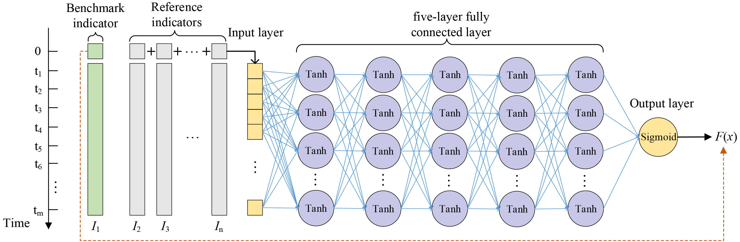

From Fig. 1, we can see that the feedforward neural network model includes: an input layer, five fully connected layers, and an output layer. Among them, the input layer indicator data is the one-dimensional vector data of the n indicators ( $I_{1},{I}_{2},\ldots,{I}_{n}$ ). All these indicators are treated as the calculation unit, and they would iterate a total of ${n}$ times. Each neuron ${c}$ in the fully connected layer can be expressed as:

$\displaystyle c=g(wx+b)$ (8)

where parameter ${x}$ denotes the input data value, ${w}$ denotes the weight, ${b}$ denotes the bias value, and $g$ denotes the activation function. Commonly used activation functions include relu, tanh, sigmoid, and so on. The relu function is a piecewise linear function. Its value is always zero on the left side of the origin and a proportional function on the right side. However, if chosen as activation function, the left derivative and the right derivative at ${x}=$ 0 are inconsistent, leading to the inability of high-order continuous differentiability. Tanh and sigmoid are infinite-order derivable functions, so using them can avoid ambiguity discussions at the origin. Further, tanh has better convergence than sigmoid. Therefore, in this paper, we use the tanh function as the nonlinear activation function. Its calculation formula is as follows.

$\displaystyle\tanh(x)=\frac{2}{1+e^{-x}}-1$ (9)

The output layer uses the sigmoid function to control the output range between zero and one. Assuming that the output after the five fully connected layers is: ( ${y}_{1},{y}_{2},\ldots,y_{k}$ ), the following output is obtained after the sigmoid layer operation:

$\displaystyle{\rm sigmoid}(y)_{i}=\frac{1}{1+\sum\limits_{j=1}^{k}e^{-(wy_{j}+% b)}}$ (10)

The objective function of the model is the mean square error (MSE). Let ${u}$ denote the number of neurons in the last fully connected layer, then:

$\displaystyle{\rm MSE}=\frac{1}{u}\sum\limits_{j=1}^{u}(y_{j}-\tilde{y}_{j})^{2}$ (11)

Then we need to select an appropriate epoch for training. We can directly obtain each neuron’s output expression $y_{h}^{q}$ in each feedforward neural network layer according to the weight and bias value after training:

$\displaystyle y_{h}^{q}=\tanh\left({\sum\limits_{g}}w_{gh}^{(p,q)}y_{g}^{p}+b_% {qh}\right)$ (12)

where $w_{gh}^{pq}$ denotes the weight of the ${g}$ th node in the ${p}$ th layer to the ${h}$ th node in the ${q}$ th layer, $y_{h}^{q}$ denotes the ${h}$ th neuron’s output value in the ${q}$ th layer, and $b_{h}^{q}$ denotes the bias value of the ${h}$ th neuron in the ${q}$ th layer. The input layer is the first layer, and the output layer is the last. In particular, when ${p}=$ 1, the following formula is satisfied:

$\displaystyle y_{h}^{p=1}=x_{h}$ (13)

When ${p}=$ 6, the following is satisfied:

$\displaystyle f(x)\buildrel\Delta\over{=}y_{h=1}^{q=7}={\rm sigmoid}\left(\sum% \limits_{g}w_{g,h=1}^{(6,7)}y_{g}^{p=6}+b_{q=7,h=1}\right)$ (14)

We have explained the calculation method of each layer. Therefore, we get the forward propagation relation ${f}({x})$ between the input and output variables.

3.4 Algorithm

Combining parts 3.2 and 3.3, we propose the calculation process, as shown in Fig. 2.

Figure 2.

Neural network and Taylor expansion application process.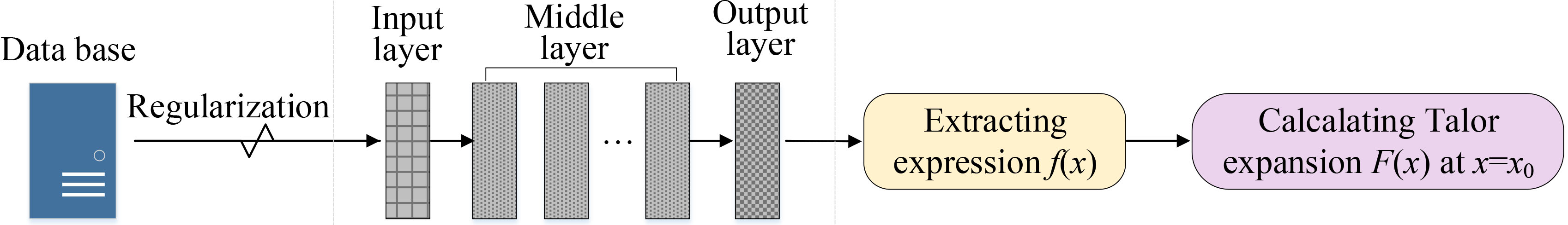

According to Fig. 2, one round of input and output calculations can obtain the multivariate correlation between the benchmark and the reference indicator. If we remove the $n$ -ary related part from the benchmark indicator and keep the remaining independent part, then the formula is obtained:

$\displaystyle f(x_{1},x_{2},\cdots,x_{n})\approx c+\lambda$ (15)

The benchmark indicator after eliminating can be regarded as a new indicator independent of the reference indicator. After a round of elimination, the database ${x}$ is updated and this process continues to iterate until there is only one indicator left. Then the database is a set of independent indicators. We assume that the number of indicators after simplification is four. The iterative process can be represented as a Venn diagram, as shown in Fig. 3.

Figure 3.

Example of the correlation elimination process using four indicators as the indicator system.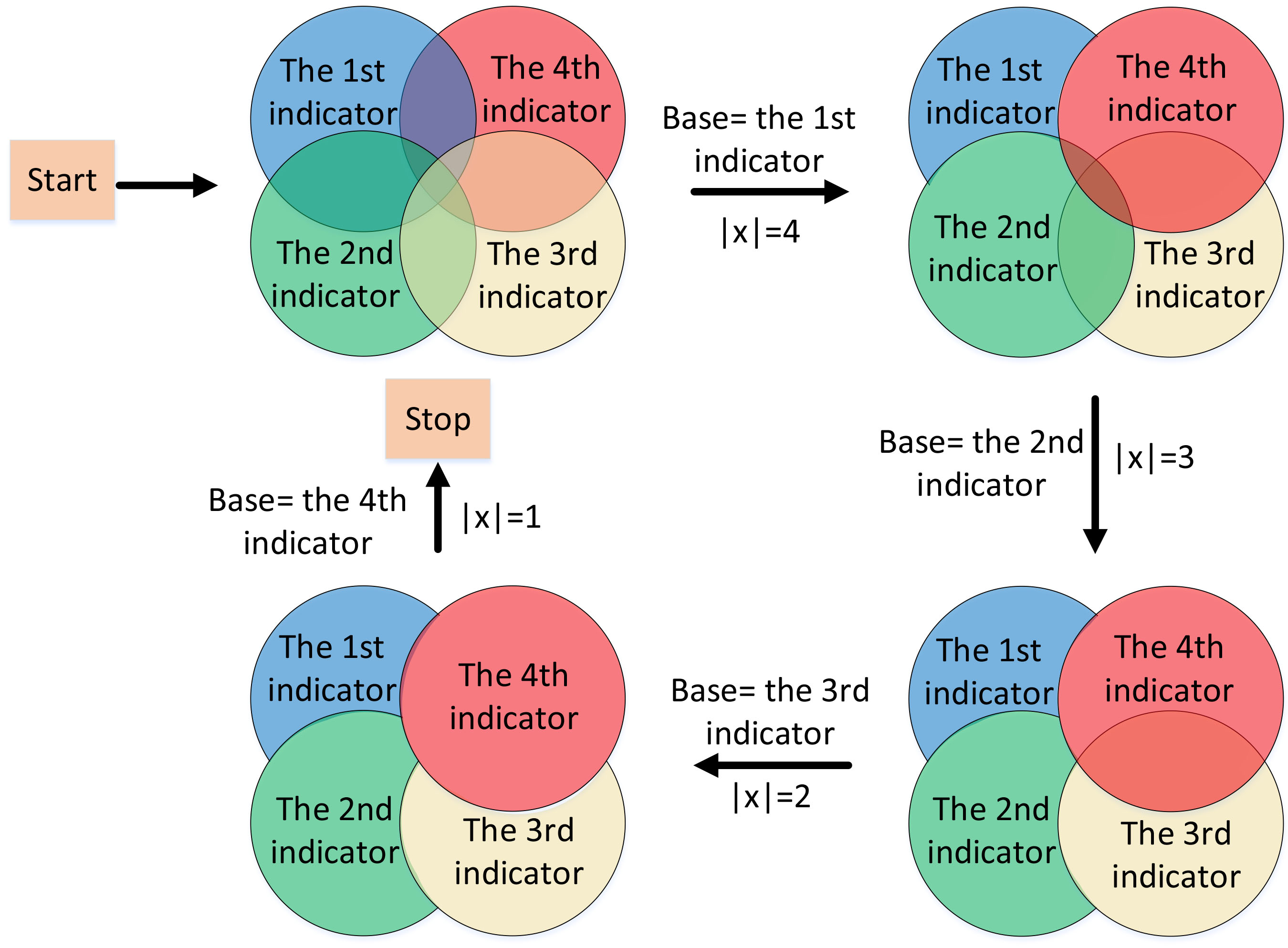

This method can visualize the abstract relationship between indicators. Each circle represents the intrinsic meaning category of the corresponding indicator, the intersection between the two circles represents the implicitly related part between the two indicators, and the intersection between the three circles represents the implicitly related part between the three indicators, and so on. If the indicator correlation elimination method is not used, the common part of the four circles will be calculated four times, the common part of the three circles will be calculated three times, and the common part of the two circles will be calculated twice. This is the reason why the evaluation effect is still not good after feature selection. The goal of our proposed method is to eliminate all these crossover parts so that each part is calculated only once. There are four steps in Fig. 3. Firstly, take indicator ${x}_{1}$ as the output of the neural network and indicator subset $\{{x}_{2},{x}_{3},{x}_{4}\}$ as the input. After the training of the neural network, the expression $x_{1}=f(x_{2},x_{3},x_{4})$ is obtained by Eq. (14) and then the expression $x_{1}=f(x_{2},x_{3},x_{4})\approx c_{1}+\lambda_{1}$ is calculated by the Taylor expansion. Thus, we have separated indicator ${x}_{1}$ from the full set of indicators. Secondly, suppose indicator ${x}_{2}$ is the output of the neural network and indicator subset $\{x_{3},x_{4}\}$ is the input of the neural network. Then the expression $x_{2}=f(x_{3},x_{4})$ is obtained after training and $x_{2}=f(x_{3},x_{4})\approx c_{2}+\lambda_{2}$ is calculated by Taylor polynomial expansion. By doing this, we have stripped indicator $x_{2}$ from the indicator subset $\{{x}_{2},{x}_{3},{x}_{4}\}$ . This process continues to iterate until there is only one indicator in the indicator subset, at which point the indicator set $\{{x}_{1},{x}_{2},{x}_{3},{x}_{4}\}$ is mutually independent indicators.

The final stop sign of correlation elimination between indicators is that the length of the current indicator set ${x}$ is one. The correlation processing algorithm based on NNTE is obtained as Algorithm 1.

Algorithm 1: Indicators’ Correlation Elimination Algorithm based on Feedforward Neural Network and Taylor Expansion (NNTE)
Input: Indicator set ${I}=\{{I}_{1},{I}_{2},\ldots,{I}_{n}\}$ , original dataset ${x}=\{{d}_{1},{d}_{2},\ldots,{d}_{n}\}$ collected at ${m}$ continuous time points
Output: Mutually independent indicator set $\tilde{I}=\{{I}_{1},{I}_{2},\ldots,{I}_{n}\}$
1: Initialize dataset ${x}=\{{d}_{1},{d}_{2},\ldots,{d}_{n}\}$ , where element ${d}_{ij}$ of the vector ${d}_{i}$ denotes the data value of this indicator at
time $j$ . $1\leqslant{j}\leqslant m$ , $\textit{index}=0$ ;
2: Normalize indicator set $\tilde{x}=\{\tilde{d}_{1},\tilde{d}_{2},\cdots,\tilde{d}_{n}\}\cong x$ ;
3: Set $x_{\min}=d_{1},x=x-d_{\min},k=6-\textit{index}$ , $c_{r}$ is the number of neurons in the r th fully connected layer;
4: Set base indicator $x_{\textit{base}}=x_{\min}$ , reference indicator $x_{\textit{refer}}={x}$ ;
5: for ( $\textit{epoch}=1$ ; $\textit{epoch}\leqslant\delta$ ) do
6: for ( ${j}=1$ ; ${j}\leqslant m$ ; ${j}++$ ) do
7: $\textit{iteration}=0$ , $x_{j}=(x_{\textit{base},j},x_{\textit{refer},{j}})$ ;
8: Bring $x_{j}$ into the Eq. (14) and calculate;
9: $\textit{iteration}++$ ;
10: $\textit{epoch}++$ ;
11: Save neural network weight $w_{gh}^{pq}$ and bias $b_{qh}$ ;
12: for ( ${h}=1$ ; ${h}\leqslant{m}$ ; ${h}++$ ) do
13: $y_{h}^{p=1}=x_{j}^{(h)}$ ;
14: for ( $q=2$ ; ${q}\leqslant{k}$ ; ${q}++$ ) do
15: for ( ${h}=1$ ; ${h}\leqslant c_{q}$ ; ${h}++$ ) do
16: $y_{h}^{q}=\text{tanh}\left(\sum_{g}w_{gh}^{p,q}y_{g}^{p}+b_{qh}\right)$ ;
17: $f(x)=\text{sigmoid}\left(\sum_{g}w_{g,h=1}^{p=k,q=k+1}y_{g}^{k}+b_{q=k+1,h=1}\right)$ ;
18: for ( ${h}=1$ ; ${h}\leqslant{m}$ ; ${h}++$ ) do
19: $x_{\textit{refer}}^{(h)}=x^{(h)}$ ;
20: $f(x^{(h)})\approx a_{1}^{(h)}x+a_{2}^{(h)}x^{2}+\cdots+a_{m}^{(h)}x^{m}+(c+% \lambda)_{\min}^{(h)}$ , where $(c+\lambda)_{\min}^{(h)}$ is the white noise value that
minimizes $f(x^{(h)})$ , $m$ denotes the highest expansion order. $m\leqslant 7$ ;
21: $f(x^{(h)})=x\sum_{h}a_{1}^{(h)}/h+x^{2}\sum_{h}a_{2}^{(h)}/h+\ldots+x^{m}\sum_% {h}a_{m}^{(h)}/h+\sum_{h}(c+\lambda)_{\min}^{(h)}/h$ ;
22: $\textit{index}++$ ;
23: $X_{\textit{index}}=(c+\lambda)_{\min}$ ;
24: if $\|x\|==1$ then
25: Output $X_{\textit{index}+1}=x$ ;
26: end
27: for ( ${i}=2$ ; ${i}\leqslant\|x\|;i++$ ) do
28: $d_{i}-1=d_{i}$ ;
29: return to step3

There are four critical procedures in the above algorithm. The first procedure (1 ${\sim}$ 11) is the calculation part of the weight and bias. Expression calculation is processed in the second procedure (12 ${\sim}$ 17). The third procedure (18 ${\sim}$ 23) is through Taylor Expansion to solve the benchmark indicator’s independent part about the reference indicator. The last procedure (24 ${\sim}$ 29) is the iterative judgment part. Through $n-1$ calculations, we can obtain a set of mutually independent indicators corresponding to the original indicators.

4. Experiment

We use crossing realm open datasets as the processing objects to reduce the impact of the one-sidedness of datasets’ choice. In cardiology, we have chosen the Cleveland dataset [11], which is widely used in machine learning. In the field of network security, we have chosen the popular KDD99 dataset [50] for DDoS evaluation. Moreover, the validity verification of the elimination algorithm may be affected by the evaluation algorithm. Therefore, we compare the results under different evaluation algorithms. We choose the classic GRA and the TOPSIS evaluation methods as the uncertainty evaluation algorithm, the WSM and WPM widely used in the industry as the deterministic evaluation algorithm.

What’s more, the tested results’ validity is affected by the incomplete selection of the elimination algorithm for comparison. To reduce this influence, we have fully classified the existing elimination algorithms in the introduction. We also adopt the widely recognized and used elimination algorithm as the comparison object (including INL, OFS, IWR, ICA, PCA, LR, and MLP). Finally, to verify the proposed algorithm’s effectiveness, we compare NNTE with other elimination algorithms’ performance by calculating the distance to the benchmark. Figure 4 shows the overall experimental flow design.

Figure 4.

Design of the experimental process of the validity of the indicator correlation elimination algorithm.

4.1 Measurement

To minimize the impact of different evaluation algorithms on the evaluation results, we have adopted four classic evaluation methods to solve the final evaluation value. Among them, the traditional GRA algorithm usually sets the distinguishing coefficient $\alpha$ to 0.5 [14], and its calculation formula is as follows:

$\displaystyle{\rm\xi}_{0i}(t)=\frac{\Delta(\min)+\alpha\Delta(\max)}{\Delta_{0% i}(t)+\alpha\Delta(\max)}$ (16)

where ${\rm\xi}_{0i}(t)$ is the gray relational coefficient of indicator sequence $x_{i}$ and the reference indicator sequence ${x}_{0}$ at time $t$ .

We suppose the indicator dataset is the matrix $X=(X_{ij})_{n*m}$ , and there are ${n}$ moments and ${m}$ evaluation indicators. The formula calculating the distance between the ${i}$ th moment and the optimal or worst moments in the TOPSIS method is as follows:

$\displaystyle D_{i}^{\max}=\sqrt{\mathop{\sum}\limits_{j=1}^{m}(Z_{\max\cdot j% }-Z_{i\cdot j})^{2}},D_{i}^{\min}=\sqrt{\mathop{\sum}\limits_{j=1}^{m}(Z_{\min% \cdot j}-Z_{i\cdot j})^{2}}$ (17)

Thus, the proximity of the ${i}$ th moment to the optimal moment is obtained as:

$\displaystyle C_{i}=\frac{D_{i}^{\min}}{D_{i}^{\max}+D_{i}^{\min}}$ (18)

The WMS requires evaluators to set the evaluation weight of each indicator in advance based on expert opinions. We suppose the value of the indicator $X_{i}$ at time $t$ is $x_{i}^{t}$ , and the weight is $a_{i}$ . Then the calculation formula of the evaluation result at time ${t}$ is as follows:

$\displaystyle S_{t}=\mathop{\sum}\limits_{i=1}^{m}a_{i}x_{i}^{t}$ (19)

Further, the solution formula of the WPM is as follows:

$\displaystyle S_{t}=\mathop{\prod}\limits_{i=1}^{m}(x_{i}^{t})^{a_{i}}$ (20)

What is more, we propose sorting accuracy (SA) to measure the similarity between the test and the expected sequence order. Its definition is as follows:

$\displaystyle SA=\frac{{\rm num}({\rm BASE}\cap{\rm AFT})}{C_{t}^{2}}$ (21)

where the numerator ${\rm num(BASE}\cap{\rm AFT)}$ denotes the number of the same sorted pairs between the benchmark sequence BASE and the processed sequence AFT, the denominator $C_{t}^{2}$ denotes the combination of two elements from ${t}$ evaluation results. For example, we suppose that the BASE ranking is ${A}>{B}>{C}$ , and the AFT ranking is ${A}>{C}>{B}$ . Then ${A}>{B}$ and ${A}>{C}$ are still the correct ranking pair, whereas $B>{C}$ is the wrong ranking pair. According to Eq. (21), the ranking accuracy rate is 2/3.

4.2 Experimental method design

The experimental method is designed according to the three levels: “dataset * evaluation algorithm * elimination algorithm.” We verify the experiment on two real public datasets (Cleveland and KDD99 datasets). And we evaluate the elimination effects of the seven comparison methods and the proposed method under four evaluation algorithms and compare their performance.

First, we set up a blank control group. This group does not use the elimination algorithm to process the dataset. We calculate the dataset’s correlation under a specific evaluation algorithm and compare the current evaluation result ranking with the benchmark. The sorting accuracy of the blank control is then calculated according to Eq. (21).

Secondly, we set up a control group. We process the dataset according to different indicator correlation elimination algorithms, including INL, OFS, IWR, ICA, PCA, LR, and MLP. To control the variables, it is consistent with the evaluation algorithm selected in the blank control group. When using INL as the elimination algorithm, we set the number of indicators to 1 ${\sim}$ max-1 to solve the sorting accuracy in turn. The next one is OFS. We utilize a specific benchmark (such as Pearson’s coefficient) to calculate the correlation between indicators. Further, we also use an iterative method to reduce the dimension. For IWR, the same baseline as OFS is used to calculate the correlation coefficient. In addition, the indicator weight is modified based on this coefficient to solve the sorting accuracy after elimination. We also use the classic ICA and the improved FastICA to test separately and keep the number of hidden factors consistent with the original indicator system. For PCA, we use the classic PCA and the improved WemPCA to test separately. The number of principal components gradually rises from one and maintains a cumulative contribution rate of more than 85%. For LR, we predict the evaluation results based on linear regression and calculate the sorting accuracy. For MLP, we use the CNN structure to fit and calculate its accuracy.

Finally, we set up the experimental group. The sorting accuracy is calculated under the NNTE method. Further, we compare and analyze the reduction efficiency of final sorting results with the other seven methods.

4.3 Heart disease

Heart disease is the biggest killer of human health in most countries. In cardiology, research on its leading causes and manifestations has become an important medical topic. It is noteworthy that classification and prediction methods based on machine learning provide new ideas for the correlation analysis of indicators of heart disease incidence.

4.3.1 Database processing

The Cleveland dataset is a well-known public dataset in this field. It contains 303 items consisting of 76 attributes related to heart disease. This dataset is available in the open database of the University of California Irvine [11]. This dataset has been marked with the evaluation results to facilitate research.

Affected by the subjective and objective factors in the collection process, there are default data in the six items of the Cleveland dataset, of which four are feature ca and two are feature thal, and the default item only accounts for 2%. Considering that the use of these six data items requires artificial data filling, additional subjective factors will be introduced. And the default items are relatively small, so the overall distribution of the data will not be affected if they are not used. Therefore, to simplify the calculation, we have deleted these default data items. Further, we extracted the relevant 14 attribute feature subsets as the research dataset [49], shown in Table 3.

Table 3
Fourteen indicators that are strongly related to heart disease in the Cleveland dataset

Indicator name	Feature description
Age	Age in years
Sex	Male or female
Cp	Chest pain type
Trestbps	Resting blood pressure
Chol	Serum cholestoral
Fbs	Fasting blood sugar
Restecg	Resting electrocardiographic results
Thalach	Maximum heart rate achieved
Exang	Exercise induced angina
Oldpeak	ST depression induced by exercise
Slope	The slope of the peak exercise ST segment
Ca	Number of major vessels (0-3) colored by flourosopy
Thal	Pathological state
Num	Diagnosis of heart disease

Paper [29] pointed out that the risk level of heart disease (the last attribute) can be predicted based on the first 13 attributes’ comprehensive evaluation. Therefore, in this experiment, our indicator system is composed of 13 attribute indicators. The main goal is to observe the impact of the indicator correlation elimination strategy on the evaluation results’ ranking.

4.3.2 Results and analysis

In the blank control group, we did not use any indicator correlation elimination strategy. Then it was evaluated based on the GRA algorithm, and the result is shown in Fig. 5. The total number of indicator pairs is 43956, and the number of ranking pairs same as the benchmark is 23818, so the ranking accuracy when using blank control is 54.186%. This probability is close to 50%, showing a lousy reduction effect. The reason for this situation is mainly due to repeated calculations between indicators. For example, the older the residents, their metabolic ability to digest and decompose glucose has decreased, so the fasting blood sugar content is more likely to be higher. Therefore, for the two indicators of age and fbs, the implicit correlation between them has been calculated more than once, which impacts the result.

Figure 5.

Evaluation results of non-correlation elimination under GRA.

Figure 6.

Comparison of different numbers of evaluation results using INL under GRA. (a) one indicator and two indicators. (b) three indicators and four indicators. (c) five indicators and six indicators. (d) seven indicators and eight indicators. (e) nine indicators and ten indicators. (f) eleven indicators and twelve indicators.

Figure 6.

Continued.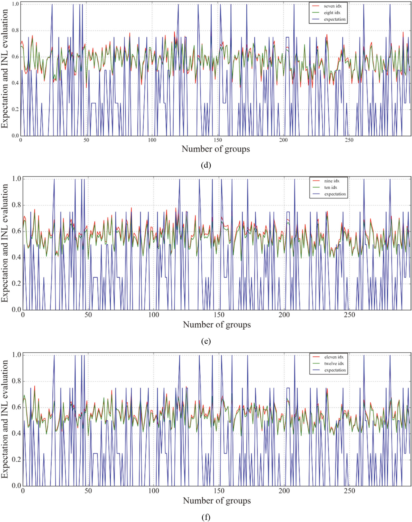

Figure 7.

Evaluation accuracy of INL and OFS strategies under GRA. (a) INL. (b) OFS.

Figure 8.

Indicator restoration results based on FastICA.

Figure 9.

Indicator restoration result based on WemPCA. (a) one principal component. (b) two principal components. (c) three principal components. (d) four principal components. (e) five principal components.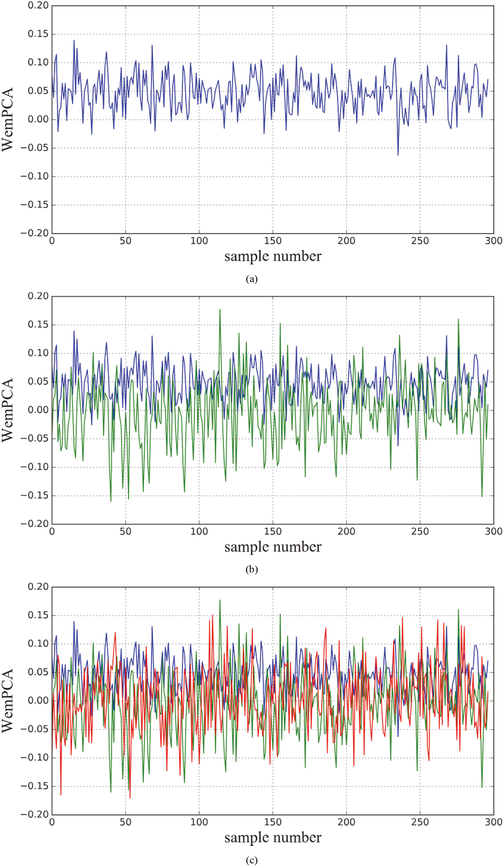

Figure 9.

Continued.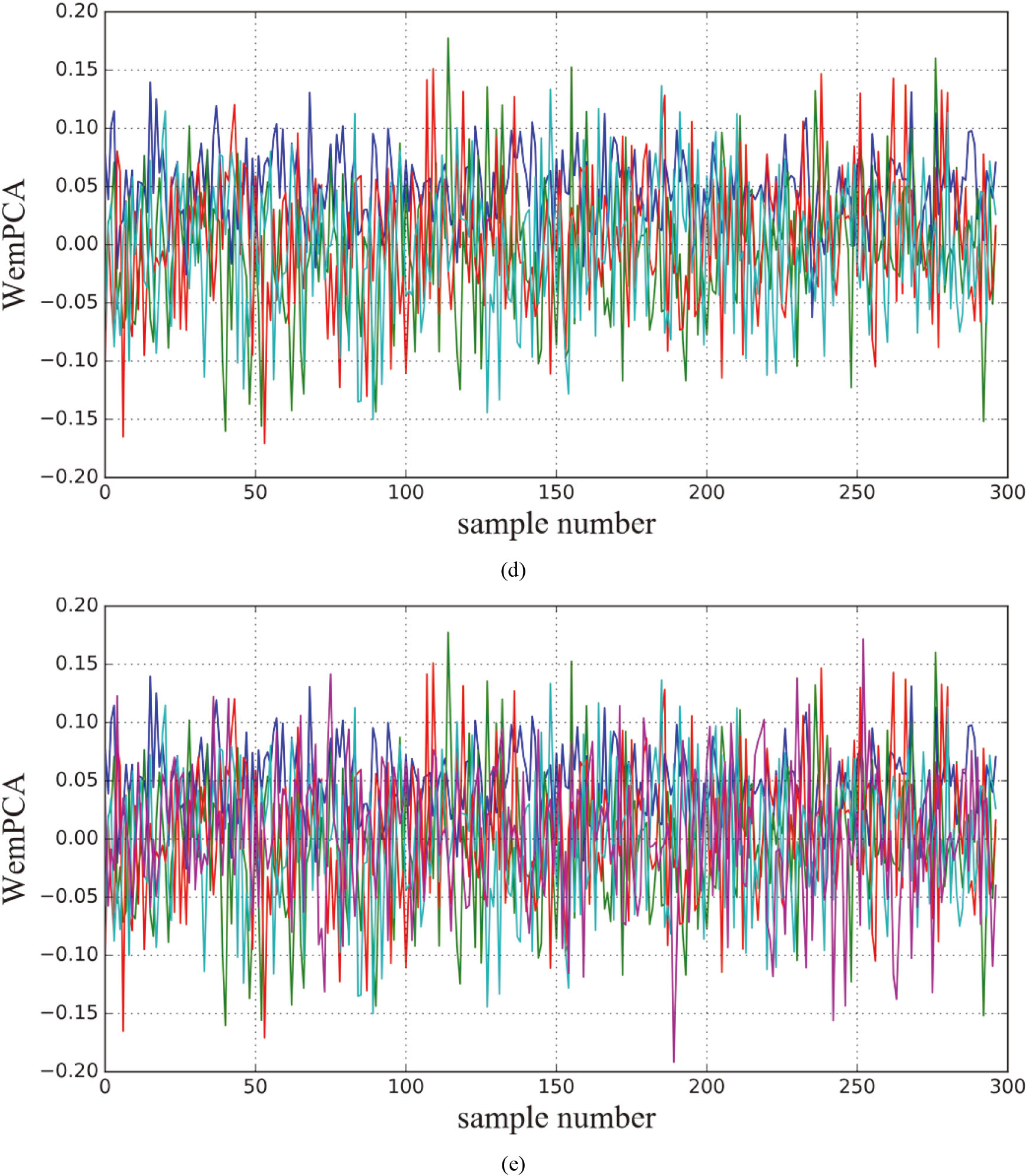

Figure 10.

Comparison of evaluation results and expectations using the NNTE algorithm under GRA.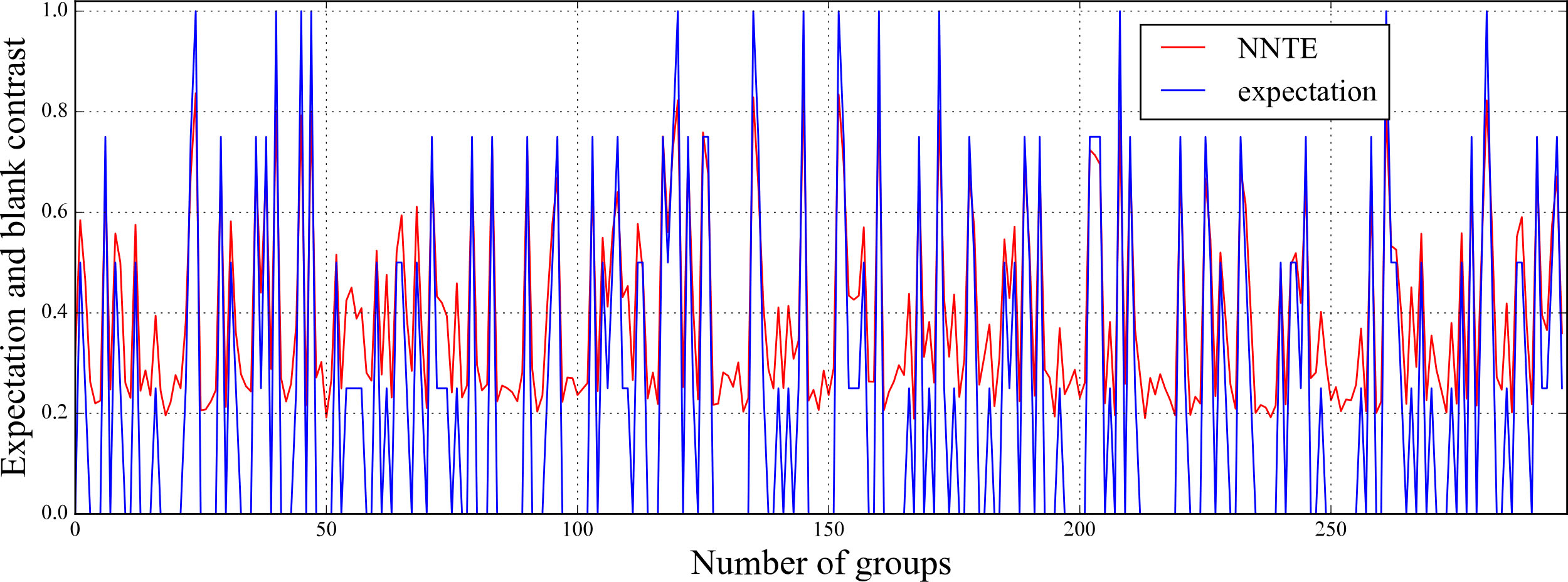

Secondly, we analyzed the evaluation result under INL. The result is shown in Fig. 6. It can be seen from this figure that as the number of indicators increases, the result becomes more stable.

We also calculate the accuracy rate changes under different numbers of indicators, and the results are shown in Fig. 7a. It shows that when the number of indicators is one to five, the sorting accuracy gradually goes up with the increase of the number of indicators. At this time, comprehensiveness is the main factor. However, when the number of indicators increases to 6 ${\sim}$ 8, the sorting accuracy gradually decreases. The situation is attributed to the large redundancy, which has a specific impact on the result. If the number of indicators is 9 ${\sim}$ 13, the sorting accuracy and the indicator’s number are positively correlated. It reaches the global maximum point peak2 when the number of indicators is 13. We also noticed another local maximum point peak1. Although peak1 is lower than peak2, the values when the indicator number is 6 ${\sim}$ 11 are all smaller than the value when the indicator number is five. That is to say, in a more general indicator system, it is necessary to balance the impact of redundancy and comprehensiveness. Specifically, the number of indicators is not always the bigger, the better; sometimes, a smaller number of indicators can get better evaluation results. Under the OFS strategy, we use the Pearson coefficient to estimate the correlation between indicators. The result is shown in Fig. 7b. According to this figure, as the number of eliminations increases, the sorting accuracy also increases. The highest accuracy rate reached 57.45%, only an increase of 3.27% compared to INL. Thus, the degree of improvement is not large.

Next, we analyzed the elimination effect under IWR. The application of this strategy in the GRA is weight modification of the final average calculation. After calculation, the sorting accuracy of IWR and OFS showed similarity, and the final sorting accuracy stayed at 57.49%. We also dealt with the correlation between indicators under the classic FastICA algorithm. This algorithm uses 13 indicators as input signals. After non-Gaussization, whitening, and rotation operations, the 13 output signals obtained are shown in Fig. 8. After testing, FastICA’s sorting accuracy reached 67.82%, which is 13.64% and 10.37% higher than INL and OFS, respectively. It can be seen that when ICA is used as an indicator processing strategy, the evaluation result is better than the other two methods.

We also tested algorithm performance under PCA. The classic PCA method is good enough, but it cannot handle the dataset maxed with considerable noise. Therefore, we verified our method under Weighted Expectation Maximization Principal Component Analysis (WemPCA), as shown in Fig. 9. After calculating, WemPCA’s sorting accuracy reached 69.83%, which is slightly higher than FastICA.

We also tested the effect of correlation elimination under MLP. After testing, CNN’s sorting accuracy reaches 71.14%. This value is slightly higher than the FastICA and WemPCA. Finally, the effect of the NNTE elimination algorithm is shown in Fig. 10. The sorting accuracy of the NNTE has reached 76.41%, which is 5.27% higher than the CNN structure. During the test, we found that when the expansion order reaches four, the average error of expansion at all sample points was controlled within 0.1%. Therefore, the low-order Taylor expansion can be used to solve the correlation elimination problem between indicators.

The comparison result of different elimination algorithms and the NNTE method is shown in Fig. 11a. Furthermore, the evaluation results under other classic algorithms (such as TOPSIS, WSM, and WPM) are shown in Fig. 11b.

Figure 11.

Comparison of the sorting accuracy of different elimination algorithms under four evaluation algorithms. (a) Comparison of SA under GRA. (b) Comparison of SA under TOPSIS, WSM, and WPM.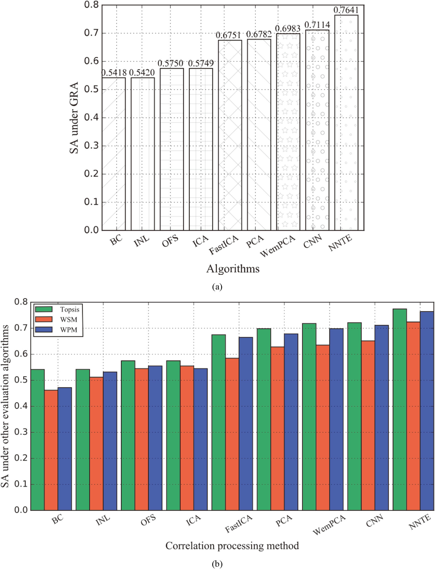

According to the above, we can conclude that the NNTE method can obtain a higher ranking accuracy under the four classic evaluation algorithms. The general applicability is also verified. However, the NNTE method is only 76.41% at the highest, still a 23.59% gap to complete ranking reduction. There are two reasons for this phenomenon. One reason is the incomplete composition of the indicator system for causes of heart disease. Although the Cleveland dataset has been widely used in all aspects of machine learning in the past few decades. Especially, the technologies in fields like prediction, classification, and correlation analysis are becoming increasingly mature. Nevertheless, few pieces of literature demonstrate and explain the completeness and objectivity of this dataset. What is more, the omission of some indicators may have a non-negligible impact on the evaluation results. The other reason attributes to the assumption that an n-party correlation exists in this paper. More specifically, regardless of the complicated functional relationship between the two indicators, we use the n-power relationship for fitting, which is consistent with the expansion nature of the Taylor expansion. However, this generalization process ignores the problem of information loss in solving the relational expressions of discrete data using continuous functions.

4.4 Network attack

The global Internet economy is developing rapidly, and so are cyber attacks. Among all the means of attack, DDoS attacks have increasingly become one of the major security threats faced by many countries and governments [34]. This type of attack has the characteristics of low threshold, low cost, high profit, and difficulty to prevent. In order to build a complete response plan, one of the keys lies in whether network security policymakers can quickly and accurately evaluate the effectiveness of DDoS attacks [24]. What is more, a good evaluation result can guide the deployment personnel to allocate limited resources in a targeted manner, thereby reducing the incident’s hazards.

4.4.1 Database processing

The KDD99 dataset is a famous network attack traffic dataset. It has five types of traffic, including normal, DoS, probing, R2L, and U2R. This dataset can be obtained from the KDD competition website held in 1999. The full data contains 4,898,431 traffic records. We extract normal traffic and DDoS-related attack traffic from the complete dataset, totaling 4,856,151 traffic records. The traffic compositions are shown in Table 4.

Table 4
Component traffic of DDoS attack

Type	Number of records
Normal	972781
Back ATK	2203
Land ATK	21
Neptune ATK	1072017
Pod ATK	264
Smurf ATK	2807886
Teardrop ATK	979

Among the six types of attack traffic, the Neptune, Smurf, and Pod attacks are based on resource consumption to overwhelm the target, while the Back, Land, and Teardrop are based on protocol vulnerabilities to attack the process of data packet interaction. In this experiment, we restrict the research object to resource exhaustion attacks. Therefore, we extract Neptune, Smurf, and Pod attacks as processing targets. Each record is composed of 42 features. According to the DDoS evaluation definition [31], the indicator system consists of four indicators, namely traffic rate, semi-connection occupancy, service occupancy, and host loss. The traffic rate indicator is calculated based on the ratio of the number of data packets sent and the duration [5], the semi-connection occupancy indicator is estimated on the percentage of connections [54], the estimated service occupancy indicator is calculated based on the percentage of service connections [36] and the host’s packet loss is calculated based on the total ratio of SYN errors and REJ errors packet rate [26]. Then, the above four performance indicators can be calculated by seven features as duration, src_bytes, dst_host_count, dst_host_same_srv_rate, dst_host_serror_rate, dst_host_rerror_rate, and type from KDD99. Then we get the evaluation indicator set. As the KDD99 dataset handles the item by assigning a real number zero when its duration is less than one second, we assume no time is crossing between records. After calculation, when we replaced zero (s) with 0.82 (s), the total flow occurred for seven days, which was consistent with the dataset description. Besides, we use 2000 items as a statistical unit and use the mean as the unit’s final evaluation result.

4.4.2 Results and analysis

The KDD99 dataset is not manually labeled. Therefore, to obtain the benchmark evaluation results, this paper uses the product of the attack duration and the number of attack packets as the attack intensity [46]. This parameter can simultaneously reflect the two dimensions of time and space and approximate the effect of DDoS attacks. The estimation result is shown in Fig. 12a. The KDD99 dataset can be divided into seven days according to the collection time. According to the attack effect from high to low, the order is 4th day $>$ 3rd day $>$ 5th day $>$ 2nd day $>$ 6th day $>$ 7th day $>$ 1st day. First of all, as a blank control, no indicator correlation processing method is used. The evaluation results obtained under the GRA are shown in Fig. 12b. It can be seen that after dividing by the number of days, the attack effect obtained from high to low is: 4th day $>$ 3rd day $>$ 5th day $>$ 7th day $>$ 1st day $>$ 2nd day $>$ 6th day. At this time, the wrong sorting pairs are 7th day $>$ 2nd day, 1st day $>$ 2nd day, 7th day $>$ 6th day, and 1st day $>$ 6th day, a total of four. Moreover, the combination is $C_{t}^{2}=21$ . So, the sorting accuracy of the blank control was (17/18) $=$ 80.952%.

Figure 12.

Estimating the attack effect through the traffic intensity and use this as the benchmark. (a) Using attack traffic intensity to calculate benchmark. (b) Evaluation results of non-correlation elimination under GRA.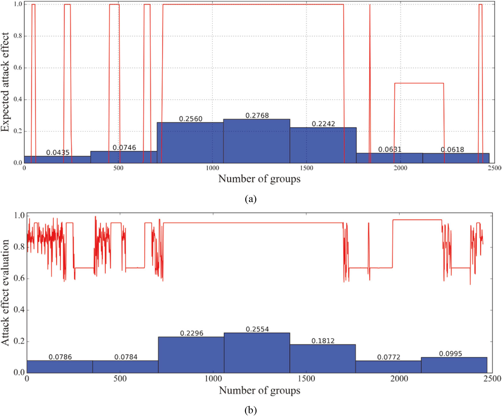

Next, we analyzed the evaluation result under INL. We selected 1 ${\sim}$ 3 indicators, respectively, as the indicator system. We also used the mean value calculation method to reduce human error. The results are shown in Fig. 13. According to this figure, as the number of indicators increases, the result ranking is closer to the benchmark.

Figure 13.

Evaluation results under different numbers of indicators when INL is adopted under GRA. (a) one indicator. (b) two indicators. (c) three indicators.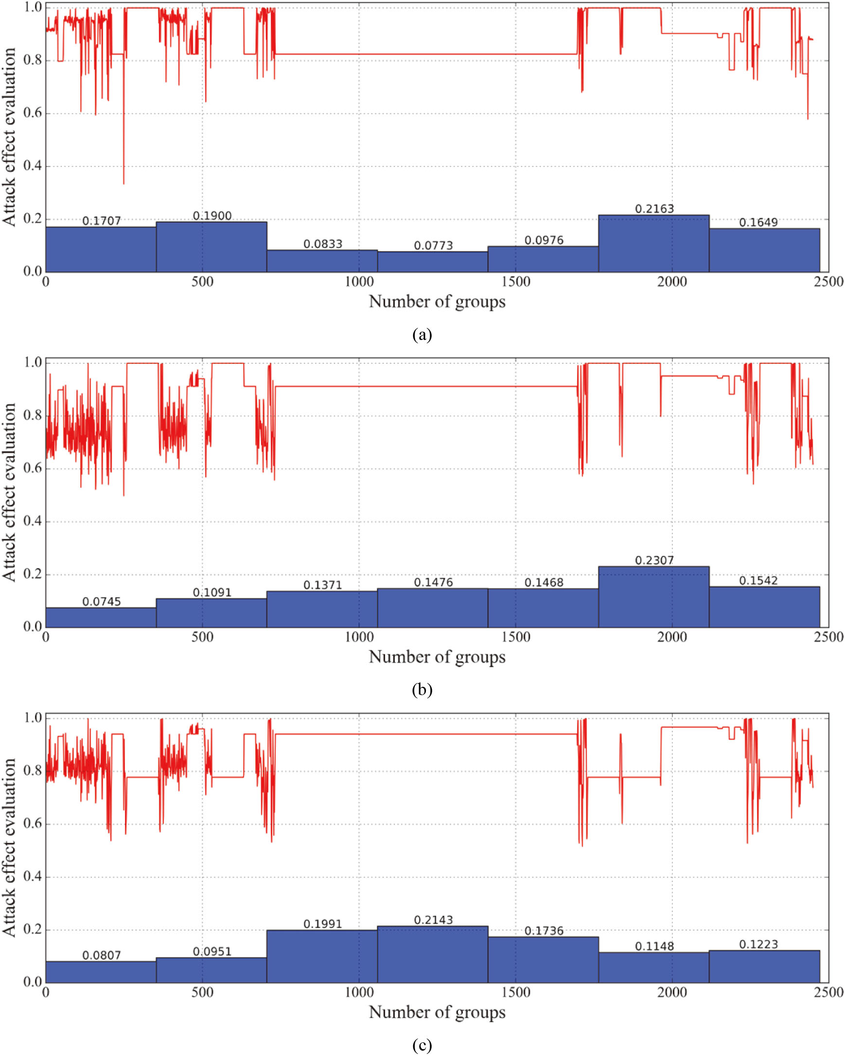

Figure 14.

Evaluation accuracy of INL and OFS under GRA. (a) INL. (b) OFS.

Figure 15.

Indicator restoration result based on FastICA.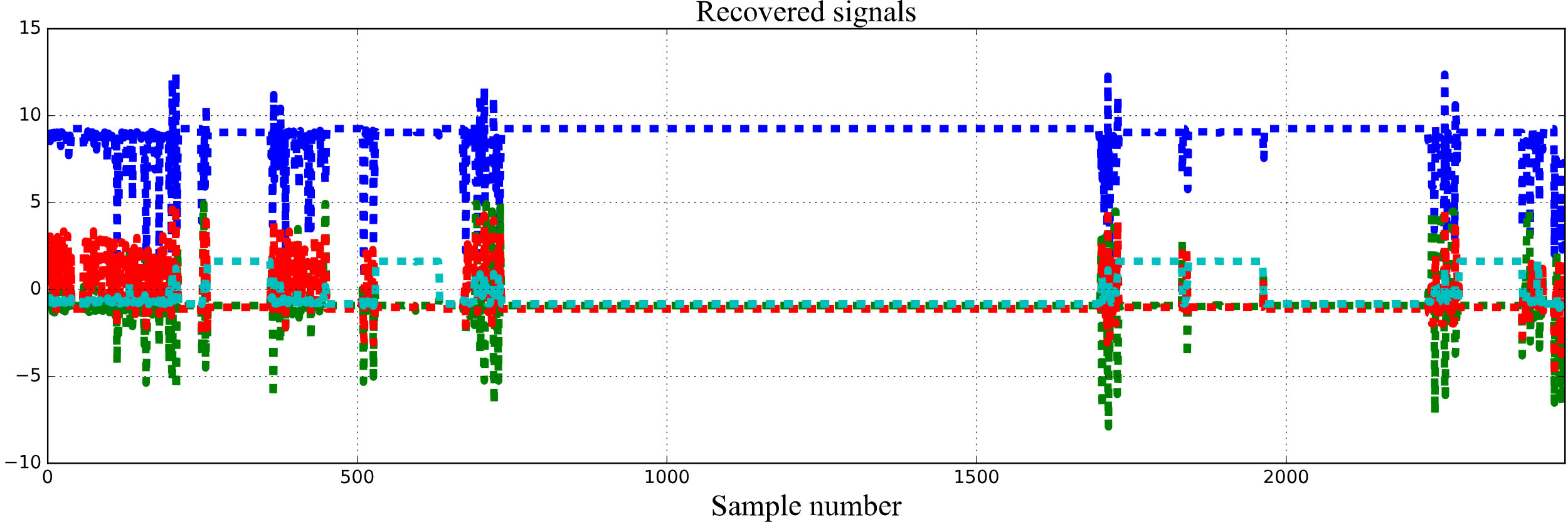

Figure 16.

Indicator restoration results based on WemPCA. (a) one principal component. (b) two principal components. (c) three principal components. (d) four principal components.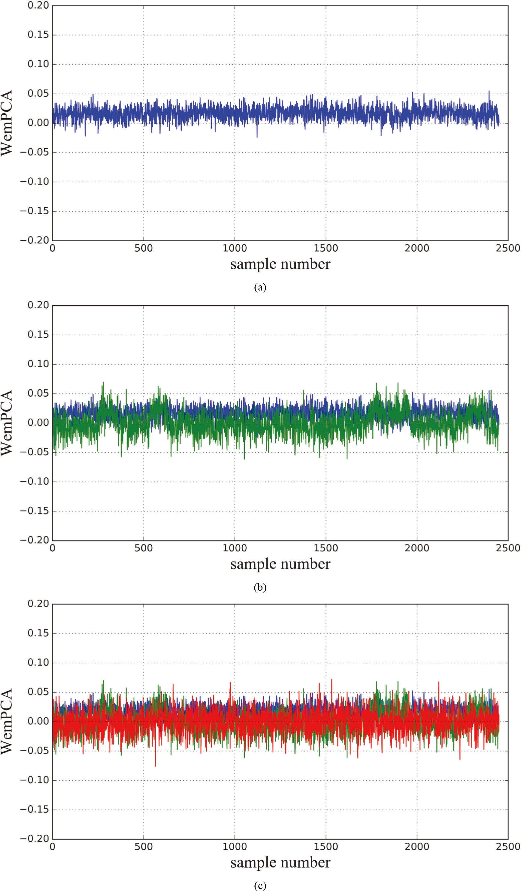

Figure 16.

Continued.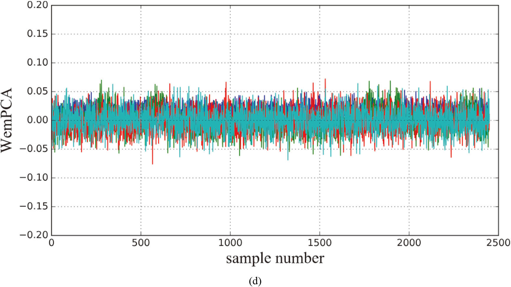

Figure 17.

Final evaluation result using NNTE elimination algorithm.

Figure 18.

Comparison of the sorting accuracy of different elimination algorithms under four evaluation algorithms. (a) Comparison of SA under GRA. (b) Comparison of SA under TOPSIS, WSM, and WPM.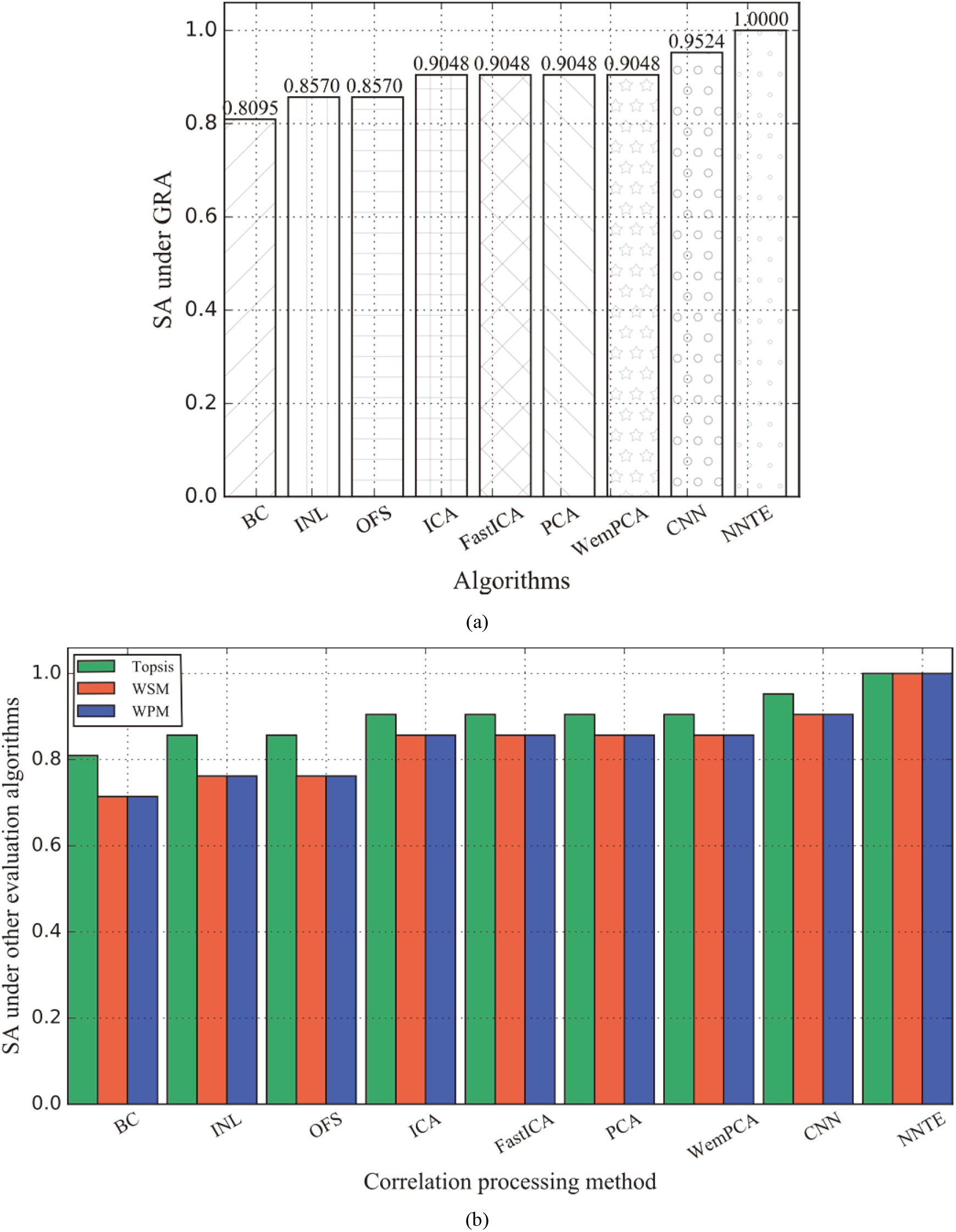

We summarized the sorting accuracy changes under different numbers of indicators, as shown in Fig. 14a. It shows that when the number of indicators is 1 ${\sim}$ 3, as the number goes up, the sorting accuracy increases. When the number of indicators is 4, the sorting accuracy starts to decrease instead. The reason is that the INL method can only balance comprehensiveness and redundancy and cannot eliminate redundant parts, leading to a double calculation of the evaluation result. Further, we measured under OFS. Similarly, we estimated the correlation between the two indicators based on the Pearson coefficient. The result is shown in Fig. 14b. We can see, as the number of iterations increases, the sorting accuracy also climbs. However, this elimination is still incomplete, with a deviation of 14.29%.

Then, we measured the method effect under the IWR. After calculation, the IWR strategy has not improved much, and the ranking accuracy is still kept at 85.71%. We also eliminated the correlation based on the FastICA algorithm. The result is shown in Fig. 15. FastICA’s sorting accuracy reached 90.476%, increasing 4.77% compared to INL and OFS.

We verified the performance under WemPCA. We calculated according to the number of principal components 1 ${\sim}$ 4, respectively. The result is shown in Fig. 16. When the number of principal components is 4, the cumulative contribution rate reaches 90%. After calculation, WemPCA’s sorting accuracy reached 90.476%, which is consistent with FastICA.

We also carry out indicator correlation elimination under the MLP. The sorting accuracy is 95.238%, which is slightly higher than FastICA and WemPCA. However, the sorting pair [7th day $>$ 1st day] cannot be correctly restored. Finally, we processed the correlation between the four indicators according to the NNTE algorithm. The final evaluation result is shown in Fig. 17. At this time, the sorting accuracy has reached 100%, which is 4.76% higher than that of the MLP method. This proposed method does not change the original indicator system composed of four evaluation indicators and effectively reduces the measurement error.

To summarize, the comparison result of different elimination algorithms and the NNTE method is shown in Fig. 18a. Figure 18b shows the comparative experimental results under other classic evaluation algorithms. We can see that the NNTE method can better restore the real ranking results under different evaluation algorithms, indicating that its high universality.

For the convenience of statistics, the final evaluation value in Fig. 18 is obtained by compressing the evaluation object from 4,856,151 items into the dataset’s seven-day collection period. Generally speaking, a smaller number of sequences can easily get higher performance. Therefore, although the final ranking accuracy reached 100%, it does not mean that the correlation of the indicator data contained in the dataset has been entirely eliminated.

The algorithm proposed in this paper solves the problem of eliminating the correlation between the indicators existing in the indicator set. The number of iterations is consistent with the number of indicators in the indicator set, and it is much lower than the power function level calculation time cost based on the mutual information algorithm. However, when the number of indicator sets is large, such as over 10,000, the computational complexity will still reach an unaffordable level [22]. In this case, professional domain knowledge can play an important role in limiting the scope of the indicator set to a smaller scope. For example, when a network security administrator evaluates the effect of a network attack, it will be based on a comprehensive set of network attack indicators. However, when a certain form of attack is known, the indicators can be screened according to the characteristics of the attack. For example, network attacks based on vulnerability exploitation do not generate large attack traffic. Unlike DDoS attacks, indicators that reflect traffic attributes can be ignored, which can reduce the number of indicators to be processed. Further, the target of an attack based on vulnerability exploitation may be the software and hardware of the attacking host [21], or it may be important information [2]. The former uses indicators that reflect host performance, including CPU occupancy, memory utilization, and storage space utilization, etc.; the latter uses indicators that reflect the value of data, including database sensitive information, file system sensitive information, and application program sensitive information, etc. In a single attack form, these two types of indicators are not related to each other. Therefore, in the beginning, we should discuss the two indicator sets separately to avoid the additional overhead caused by the cross calculation of the two subsets.

5. Conclusion

In this article, we proposed a new correlation elimination method for processing the overlap between multiple indicators. We also discussed the possibility of combining the feedforward neural network with the Taylor expansion. Further, we designed a hierarchical stripping method to reduce the dimensionality of the indicator set effectively. Specifically, the feedforward neural network is used to fit the functional relationship between the input and the output variable. The functional relationship is then expanded by the Taylor series at different sample points to obtain independent partial sequences. The sequence can also be expanded in the time dimension. The experimental results show that the indicator correlation elimination algorithm based on the NNTE can effectively solve the evaluation result ranking misalignment caused by the nonlinear correlation between the indicators. It may help evaluators choose appropriate countermeasures based on the evaluation results.

6. Future research

We have verified the feasibility and effectiveness of our proposed method based on two datasets. Nevertheless, there still exist the following problems:

Question 1. This paper’s work is based on the assumption that there is a continuous function relationship between each indicator variable. However, this assumption ignores the problem of information loss in the process of indicator data transformed from discrete form to continuous form. Therefore, in the next research, we need to design a strategy for eliminating correlations between discrete indicator data. Question 2. This paper’s algorithm has two key operations: Neural network solving expressions and Taylor expansion to eliminate errors. The former depends on the structure of the neural network and tuning parameters. Therefore, different model layers and parameter settings may have a great impact on the final result. The latter depends on the order of Taylor expansion at different discrete points. The expansion under different orders has different effects on the error. Therefore, it is necessary to design an optimization algorithm that can adaptively select the network structure and expansion order according to the dataset. Question 3. The second experiment used days as the evaluation unit for the convenience of calculation. This division is not only subjective but also leads to distortion of accuracy. So in the next research, items should be chosen as the evaluation unit. Moreover, efficient data processing methods should be proposed to visualize millions of items.

Footnotes

Acknowledgments

We thank our colleagues of the Information Engineering University’s Evaluation Theory and Analysis group for fruitful discussions. Mainly, Han Qiu patiently guided this paper.

Conflict of interest

The authors declare that there is no conflict of interest regarding the publication of this paper.

Funding statement

The authors received no specific funding for this study.

References

Hyvarinen

, Fast ICA for noisy data using gaussian moments, Proc. – IEEE Int. Symp. Circuits Syst. 5 (1999), 57–61.

Stasinopoulos

Ntantogian

and Xenakis

, Commix: Automating evaluation and exploitation of command injection vulnerabilities in Web applications, Int. J. Inf. Secur. 18(1) (2019).

Billah

King

M.L.

Snyder

R.D.

and Koehler

A.B.

, Exponential smoothing model selection for forecasting, Int. J. Forecast. 22(2) (2006).

B¨ttcher

Keller-Ressel

and Schilling

R.L.

, Distance multivariance: New dependence measures for random vectors, Ann. Stat. 47(5) (2019), 2757–2789.

Buragohain

and Medhi

, FlowTrApp: An SDN based architecture for DDoS attack detection and mitigation in data centers, 2016.

Perrotta

and Williamson

, The social life of Learning Analytics: Cluster analysis and the “performance” of algorithmic education, Learn. Media Technol. 43(1) (2018).

Fitz-Gibbon

C.T.

, Multilevel Modelling in an Indicator System, in: Schools, Classrooms, and Pupils, London, 1991, pp. 67–83.

Nguyen

and Eisenstein

, A Kernel independence test for geographical language variation, Comput. Linguist. 43(3) (2017), 567–592.

Matteson

D.S.

and Tsay

R.S.

, Independent component analysis via distance covariance, J. Am. Stat. Assoc. 112(518) (2017), 623–637.

10.

Hosmer

D.W.

Lemeshow

and Sturdivant

R.X.

, Applied Logistic Regression: Third Edition, 2013.

11.

Aha

D.W.

, Machine Learning Repository: Heart Disease Data Set, Uci, 1988. https://archive.ics.uci.edu/ml/datasets/heart+Disease.

12.

Forsythe

and Wu

J.-C.

, Explaining Demographic Heterogeneity in Cyclical Unemployment, Pap. under Rev. requested, Labour Econ., 2019.

13.

Fan

Zhong

Yan

and Yue

, A hybrid fuzzy evaluation method for curtain grouting efficiency assessment based on an AHP method extended by D numbers, Expert Syst. Appl. 44 (2016).

14.

Wei

G.W.

, GRA method for multiple attribute decision making with incomplete weight information in intuitionistic fuzzy setting, Knowledge-Based Syst. 23(3) (2010), 243–247.

15.

Bourlard

and Kamp

, Auto-association by multilayer perceptrons and singular value decomposition, Biol. Cybern. 59(4–5) (1988), 291–294.

16.

Cui

and Zhong

, A distribution-free test of independence based on mean variance index, Comput. Stat. Data Anal. 139 (2019), 117–133.

17.

Peng

Long

and Ding

, Feature selection based on mutual information: Criteria of max-dependency, max-relevance, and min-redundancy, IEEE Trans. Pattern Anal. Mach. Intell. 27(8) (2005).

18.

Kim

I.Y.

and De Weck

O.L.

, Adaptive weighted-sum method for bi-objective optimization: Pareto front generation, Struct. Multidiscip. Optim. 29(2) (2005).

19.

Wright

J.D.

, Address unknown: The homeless in America, 2017.

20.

Zar

J.H.

, Significance testing of the spearman rank correlation coefficient, J. Am. Stat. Assoc. 67(339) (1972), 578–580.

21.

Jang-Jaccard

and Nepal

, A survey of emerging threats in cybersecurity, in: Journal of Computer and System Sciences, Vol. 80, no. 5, 2014.

22.

et al., Feature selection: A data perspective, ACM Computing Surveys 50(6) (2017).

23.

Bevan

J.M.

and Kendall

M.G.

, Rank Correlation Methods, Stat. 20(3) (1971), 74.

24.

Mirkovic

Fahmy

and Reiher

, Measuring impact of dos attacks, Proc. DETER Community Work. Cyber Secur. Exp., 2006, 1–4, [Online]. Available: http://citeseerx.ist.psu.edu/viewdoc/download?doi=10.1.1.87.3507&rep=rep1&type=pdf.

25.

Riley

, Indicator quality for assessment of impact of multidisciplinary systems, Agric. Ecosyst. Environ. 87(2) (2001), 121–128.

26.

Wang

and bin Hou

, Packet loss rate mapped to the quality of experience, Multimed. Tools Appl. 77(1) (2018).

27.

Zhu

and Collette

, A dynamic discretization method for reliability inference in Dynamic Bayesian Networks, Reliab. Eng. Syst. Saf. 138 (2015).

28.

Yoon

K.P.

and Kim

W.K.

, The behavioral TOPSIS, Expert Syst. Appl. 89 (2017).

29.

Rani

K.U.

, Analysis of heart diseases dataset using neural network approach, Int. J. Data Min. Knowl. Manag. Process 1(5) (2011), 1–8.

30.

Zheng

Wang

and Wu

, Feature subset selection combining maximal information entropy and maximal information coefficient, Appl. Intell. 50(2) (2020).

31.

Apiecionek

Ł.

Czerniak

J.M.

and Dobrosielski

W.T.

, Quality of services method as a DDoS protection tool, Adv. Intell. Syst. Comput. 323 (2015).

32.

Albert

Bouret

Fromont

and Reynaud-Bouret

, Bootstrap and permutation tests of independence for point processes, Ann. Stat. 43(6) (2015), 2537–2564.

33.

Fischlin

, A cost-effective pay-per-multiplication comparison method for millionaires, in: Lecture Notes in Computer Science (Including Subseries Lecture Notes in Artificial Intelligence and Lecture Notes in Bioinformatics), Vol. 2020, 2001.

34.

Bhuyan

M.H.

Bhattacharyya

D.K.

and Kalita

J.K.

, An empirical evaluation of information metrics for low-rate and high-rate DDoS attack detection, Pattern Recognit. Lett. 51 (2015).

35.

Sedlmair

Tatu

Munzner

and Tory

, A taxonomy of visual cluster separation factors, Comput. Graph. Forum 31(3 PART 4) (2012), 1335–1344.

36.

Hoque

Bhattacharyya

D.K.

and Kalita

J.K.

, A novel measure for low-rate and high-rate DDoS attack detection using multivariate data analysis, 2016.

37.

Comon

, Independent component analysis, A new concept, Signal Processing 36(3) (1994), 287–314.

38.

Dos Santos

P.H.

Neves

S.M.

Sant’Anna

D.O.

de Oliveira

C.H.

and Carvalho

H.D.

, The analytic hierarchy process supporting decision making for sustainable development: An overview of applications, Journal of Cleaner Production 212 (2019).

39.

Pearson Karl, VII. Mathematical contributions to the theory of evolution. – III. Regression, heredity, and panmixia, Philos. Trans. R. Soc. London. Ser. A, Contain. Pap. a Math. or Phys. Character 187 (1896), 253–318.

40.

Ginevičius

Podvezko

and Mikelis

, Quantitative evaluation of economic and social development of lithuanian regions, Ekonomika 65 (2004).

41.

Rajesh

and Ravi

, Supplier selection in resilient supply chains: A grey relational analysis approach, J. Clean. Prod. 86 (2015).

42.

Ramadiani Ramadhani

Arifin

Jundillah

M.L.

and Azainil

, Decision support system for determining Chili land using weighted product method, Bull. Electr. Eng. Informatics 9(3) (2020).

43.

Bailey

, Principal component analysis with noisy and/or missing data, Publ. Astron. Soc. Pacific 124(919) (2012), 1015–1023.

44.

Liu

S.C.

and Liu

, Network security risk assessment method based on HMM and attack graph model, 2016.

45.

Wold

Esbensen

and Geladi

, Principal component analysis, Chemom. Intell. Lab. Syst. 2(1–3) (1987), 37–52.

46.

Tian

Guo

and Wu

D.O.

, Can we beat DDoS attacks in clouds, IEEE Trans. Parallel Distrib. Syst. 25(9) (2014).

47.

Berrett

T.B.

and Samworth

R.J.

, Nonparametric independence testing via mutual information, Biometrika 106(3) (2019), 547–566.

48.

Kim

and Adali

, Approximation by fully complex multilayer perceptrons, Neural Comput. 15(7) (2003), 1641–1666.

49.

Dulhare

U.N.

, Prediction system for heart disease using Naive Bayes and particle swarm optimization, Biomed. Res. 29(12) (2018).

50.

UCI, KDD99 Data Set, 1999. http://kdd.ics.uci.edu/databases/kddcup99/kddcup99.html.

51.

Tiwari

Jain

P.K.

and Tandon

, Product design concept evaluation using rough sets and VIKOR method, Adv. Eng. Informatics 30(1) (2016).

52.

Becker

Saisana

Paruolo

and Vandecasteele

, Weights and importance in composite indicators: Closing the gap, Ecol. Indic. 80 (2017).

53.

W.J.

and Fang

X.Y.

, Assessment of black-start modes based on entropy value method and principal component analysis, Dianli Xitong Baohu yu Kongzhi/Power Syst. Prot. Control 42(8) (2014).

54.

Wang

Guo

Gao

and Feng

, Distributed denial of service attack defence simulation based on honeynet technology, J. Ambient Intell. Humaniz. Comput., 2019.

55.

Wang

Y.M.

and Elhag

T.M.S.

, A goal programming method for obtaining interval weights from an interval comparison matrix, Eur. J. Oper. Res. 177(1) (2007).

56.

Jin

and Matteson

D.S.

, Generalizing distance covariance to measure and test multivariate mutual dependence via complete and incomplete V-statistics, J. Multivar. Anal. 168 (2018).

57.

and Hanson

T.E.

, Bayesian nonparametric test for independence between random vectors, Comput. Stat. Data Anal. 149 (2020), 106959.

An integrated model based on feedforward neural network and Taylor expansion for indicator correlation elimination

Abstract

Keywords

1. Introduction

Table 1 Classification of indicator correlation elimination

3. Methodology

3.1 N-power correlation

Table 2 Contrast with different numbers of hidden layers

4.3 Heart disease

4.3.1 Database processing

Table 3 Fourteen indicators that are strongly related to heart disease in the Cleveland dataset

4.4.1 Database processing

Table 4 Component traffic of DDoS attack

6. Future research

Footnotes

Acknowledgments

Conflict of interest

Funding statement

References

Table 1
Classification of indicator correlation elimination

Table 2
Contrast with different numbers of hidden layers

Table 3
Fourteen indicators that are strongly related to heart disease in the Cleveland dataset

Table 4
Component traffic of DDoS attack