
Abstract
Bayesian network (BN) is one of the most powerful probabilistic models in the field of uncertain knowledge representation and reasoning. During the past decade, numerous approaches have been proposed to build directed acyclic graph (DAG) as the structural specification of BN. However, for most Bayesian network classifiers (BNCs) the directed edges in DAG substantially represent assertions of conditional independence rather than causal relationships although the learned joint probability distributions may fit data well, thus they cannot be applied to causal reasoning. In this paper, conditional entropy is introduced to measure causal uncertainty due to its asymmetry characteristic, and heuristic search strategy is applied to build Bayesian causal tree (BCT) by identifying significant causalities. The resulting highly scalable topology can represent causal relationship in terms of causal science, and corresponding joint probability can fit training data in terms of data science. Then ensemble learning strategy is applied to build Bayesian causal forest (BCF) with a set of BCTs, each taking different attribute as the root node to represent root cause for causality analysis. Extensive experiments performed on 32 public datasets from the UCI machine learning repository show that BCF achieves outstanding classification performance compared to state-of-the-art single-model BNCs (e.g., CFWNB), ensemble BNCs (e.g., WATAN, IWAODE, WAODE-MI and TAODE) and non-Bayesian learners (e.g., SVM, k-NN, LR).
Introduction
Training classifier is one of the great challenges in data mining and machine learning [1]. Some state-of-the-art supervised learning algorithms (e.g., Decision Tree [2, 3], Bayesian network (BN) [4, 5], Support Vector Machine [6] and Neural Network [7]) have been introduced for learning from data. When applied to deal with classification problems, Bayesian network classifier (BNC) is much more powerful than other algorithms due to its knowledge expressivity [8, 9, 10]. The network topology of BNC and corresponding joint probability qualitatively and quantitatively describe the statistical knowledge. One of the most exciting prospects in recent years has been the possibility of using BNC to discover causal structures implicated in training data [11, 12, 13, 14] – a task previously considered impossible without controlled experiments.
Learning BNC from data includes structure learning and parameter learning. Naive Bayes (NB) [15] receives more attention from researchers around the world due to its extreme simplicity and superior performance. The network structure of NB is commonly used as the basic framework of restricted BNCs, e.g., state-of-the-art single-model BNCs (e.g., tree augmented naive Bayes (TAN) [16]) and ensemble BNCs (e.g., averaged one-dependence estimators (AODE) [17]). To improve the generalization performance and fully represent the coverage of dependency relationships implicated in training data, ensemble BNCs focus on the study of diversity among sub-classifiers and distribute the errors of base BNCs across different parts of the instance space. Any complete probabilistic model of a domain must, either explicitly or implicitly, represents the joint probability distribution of every possible event defined by the values of all the variables. BNCs achieve compactness by factoring the joint probability distribution into conditional probabilities for each variable given its parents. After learning the network structure, weighting can be applied to further improve the estimate of conditional probability for single-model BNC [18] or joint probability for each sub-classifier in ensemble BNC [19, 20, 21, 22].
Judea Pearl, who is the Turing Award winner and recognized for his work in artificial intelligence especially through the invention of Bayesian networks, proposed the idea of conversion from Big Data Revolution to Causal Science Revolution in the keynote speech “The New Science of Cause and Effect with reflections on data science and artificial intelligence” in 2020. Since our intuitive understanding is usually framed in how one variable influences another [23], it can be more helpful to reason in terms of causality in different situations, such as the study of causal dependence between time series [24, 25], analysis of the direction and frequency content of the brain activity flow [26], identification of nonlinear input-state-output systems [27] and etc [28, 29, 30]. Pearl [31] assumes directed acyclic graph (DAG) as the structural specification of causal Bayesian networks, in which the directed edges can represent directed causal relationships, pointing from cause attributes to effect attributes. However, when information theory is applied to learn the network structure of BNC from data and information-theoretic metrics (e.g., mutual information and conditional mutual information) are introduced to measure mutual dependence or conditional dependence, the arrows in the diagram represent the flow of information rather than causal connections. The learned acausal BNC represents assertions of conditional independence, whereas probabilistic independencies in themselves do not imply a causal structure and vice versa.
The contributions of this paper are introduced as follows:
We prove the reasonableness of using conditional entropy to measure the causality between attributes. Then heuristic search strategy is applied to build Bayesian causal tree (BCT) by identifying significant causalities. The resulting highly scalable topology can represent causal relationship in terms of causal science, and corresponding joint probability can fit training data in terms of data science. The interactions among variables in causal network are asymmetric and this asymmetry leads to causal ordering of the variables, which implicitly assumes that the first variable in the order is the only cause variable that no other variable influence it. To address this issue, we apply ensemble learning to build Bayesian causal forest (BCF) with a set of BCTs, each taking different attribute as the root node to represent root cause for causality analysis. We compare the classification performance of BCF with five variations of the state-of-the-art NB, TAN and AODE, including single-model BNCs (e.g., CFWNB [18]), ensemble BNCs (e.g., WATAN [20], IWAODE [21], WAODE-MI [22], TAODE [32]) and non-Bayesian learners (e.g., SVM [6], k-NN [33], LR [34]). The experimental results show that BCF demonstrates competitive classification performance in terms of zero-one loss, RMSE, F1-Score and AUC on 32 datasets with 4 to 42 attributes and 57 to 299,285 instances.
The rest of this paper is organized as follows. Section 2 reviews some information-theoretic metrics and clarifies the difference between undirected dependence and directed causality for BNC learning. Section 3 describes in detail the learning procedure of our algorithm, BCF. Section 4 presents the extensive experimental results and compares the performance of BCF with other five algorithms. At last, Section 5 shows the conclusions and puts forward the research direction of future work.
Definitions and notions
BNC is a probabilistic model designed for classification, which consists of two parts: (1) the network structure
When given a testing instance
For the joint probability distribution described in Eq. (1), restricted BNC
Each factor in Eq. (2), i.e.,
Information theory is a science that studies the law of information measurement, transmission and transformation with mathematical statistics. In this paper, entropy
.
[35] Entropy
.
[35] Conditional entropy
.
[35] Conditional mutual information (CMI)
When given an instance
where
In the following discussion, we will clarify the basic ideas of different BNCs from the perspective of dependence analysis and causality analysis.
Single-model BNC
Among all the BNCs, NB has the simplest topology due to its independence assumption that each attribute is independent of the other attributes given the class variable
NB doesn’t need to learn the network structure, and thus only the estimates of probabilities
Example of (a) KDB with 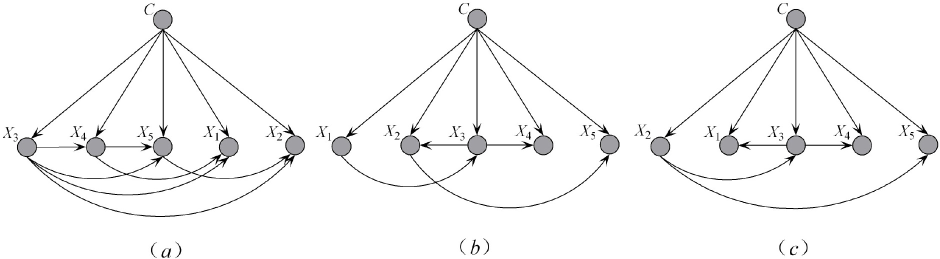
The
Roughly speaking, for causal BN each non-root node is the direct effect of its parents and the directed edges are considered to represent spontaneous causality from the cause variables to the effect variables. However, the directed edge in BN only depicts statistical dependence between variables, not necessarily corresponds to causality.
Ensemble learning is widely used to deal with classification problems and can greatly improve the classification accuracy of base classifiers. Its underlying idea is to combine multiple weak supervised learners to obtain a better and more comprehensive strong supervised learner. Even if one weak classifier gets the wrong prediction, other weak classifiers can correct the error. AODE is an ensemble of superparent one-dependence estimators (SPODEs). Figure 2 shows an example of SPODE, which chooses
By comparing Eqs (7) and (8), the independence assumption of SPODE can be regarded as an explicit variation of NB. Since SPODEs in AODE respectively take each attribute as the superparent that points to the rest of the attributes [41]. Directed edges
The topology of SPODE.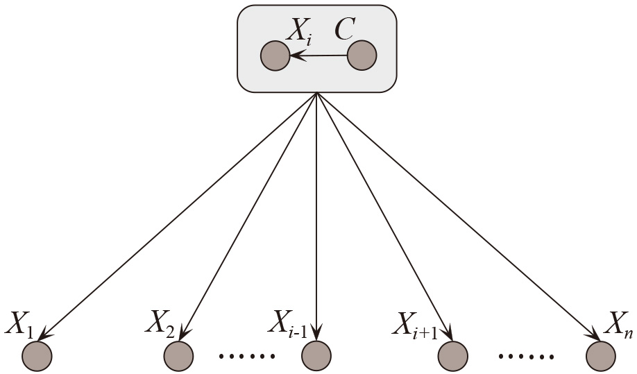
Similar to the learning strategy of AODE, ATAN [20] also selects each attribute in turn as the root node to build several different directed maximum weighted spanning trees. Directed edges
Bayesian causal tree
Information theory is widely used to identify information flow in complex systems. For BNC learning, the conditional mutual information (CMI)
The comparison between the distribution of 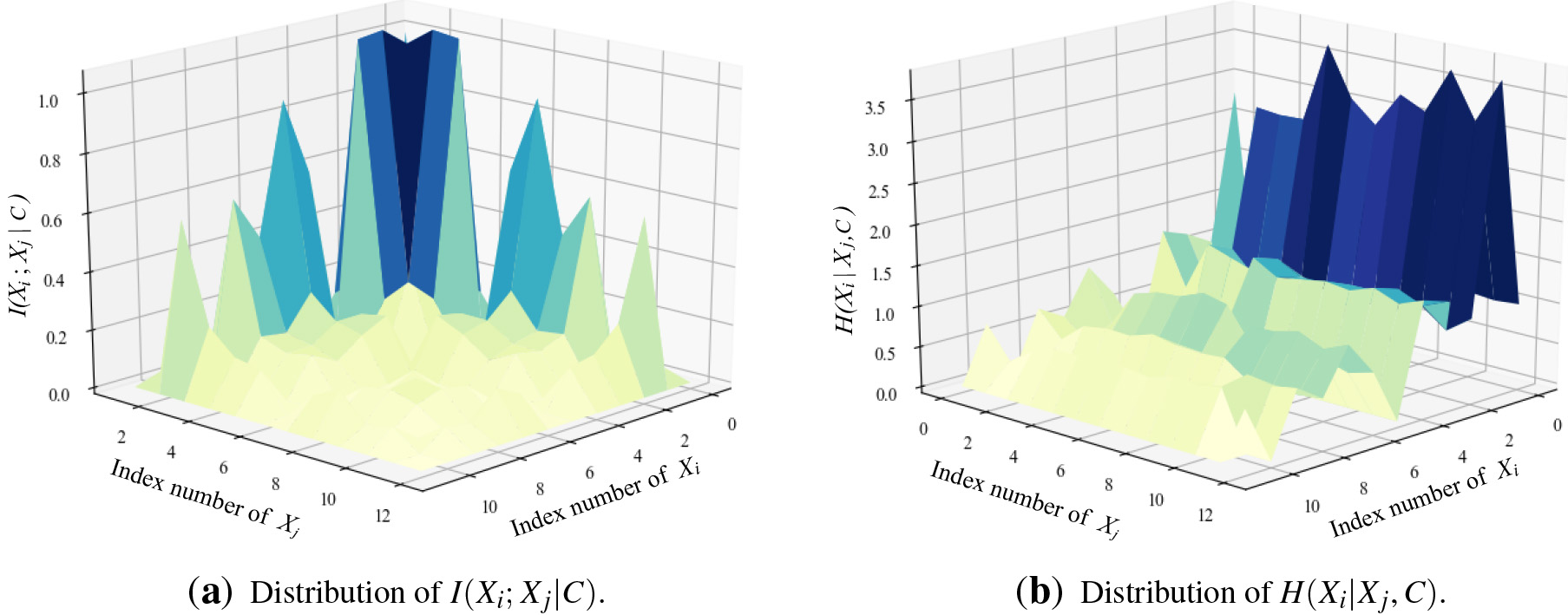
If directed edge
Each factor
Suppose that the attributes have been sorted implicitly or explicitly, and the order is
Then conditional entropy
Suppose that node
[h] BCT-Learning (
BCT builds a causal tree to identify the causal relationships with a prior root attribute as the root cause. Then the attribute order will be uniquely determined by comparing conditional entropy
Dataset Localization for experimental study
Dataset Localization for experimental study
The results of
For 1-dependence topology, each children attribute can have at most one parent attribute or each effect attribute can have at most one cause attribute. If attribute
Example of (a) BCT with 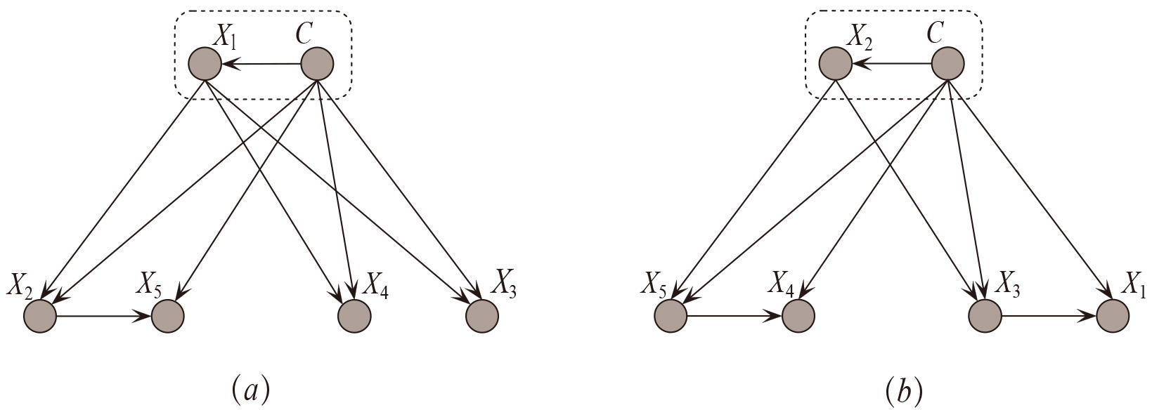
The learning framework of BCF is described in Fig. 5, and the training and testing procedures of BCF are respectively described by Algorithms 4 and 3.2. At the training phase, BCF respectively selects each attribute
BCF-Training
BCF-Test
Average the estimates of joint probabilities
The learning framework of BCF. 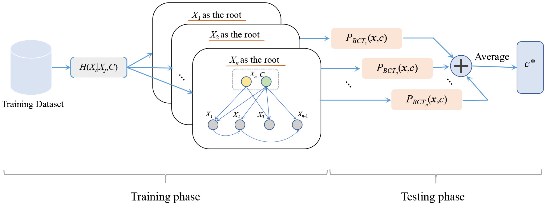
Domingos [44] pointed out that Bayesian model averaging is theoretically the optimal method for combining learned models. At the testing phase, BCF needs
where
Experimental setting and benchmark datasets
To illustrate the difference in classification performance of the algorithms being compared, we perform experiments on 32 benchmark datasets from the UCI machine learning repository [45] and record the number of instances, attributes, and classes for each dataset in Table 3. The datasets were divided into two categories, i.e., large datasets with the number of instances
CFWNB [18], correlation-based feature weighting filter for naive Bayes. WATAN [20], weighted averaged tree augmented naive Bayes. IWAODE [21], instance-based weighting filter for SPODE. WAODE-MI [22], mutual information weighted AODE. TAODE [32], targeted AODE. SVM [6], support vector machine with default parameters. LR [34], logistic regression with default parameters. k-NN [33], k-Nearest Neighbor with default parameters.
To evaluate the effectiveness and efficiency of BCF, some statistics were employed to interpret the results.
where
where
where
where
Tables A1–A3 in Appendix A respectively show the detailed results of zero-one loss, RMSE and F1-Score of all the 9 algorithms on 32 datasets. The symbols
Datasets
Zero-one loss
The W/D/L records summarizing the zero-one loss of the state-of-the-art BNCs are shown in Table 4, from which we can see that weighted AODEs perform better in terms of zero-one loss than CFWNB and WATAN. For example, TAODE beats CFWNB on 15 datasets and loses on 8, and beats WATAN on 15 datasets and loses on 5. The reason may be that whether causality
Win-Draw-Loss results of zero-one loss on 32 datasets
Win-Draw-Loss results of zero-one loss on 32 datasets
To further analyze the effectiveness of the mechanism of BCF, we present the scatter plot of zero-one loss for BCF and the other two algorithms (WATN and TAODE) in Fig. 6, where the X-axis shows the index number of datasets and the Y-axis corresponds to the values of relative zero-one loss
The sub classifiers in WTAN apply the same topology and the number of undirected edges measured by conditional mutual information is limited, that cannot help demonstrate the diversity among sub classifiers and thus weighting is the only effective approach to tune the estimate of joint probability for data fitting. In contrast, the SPODE members in weighted AODE apply different independence assumptions and corresponding network topologies vary greatly. All possible conditional dependencies or causal relationships between attributes, significant or non-significant, are fully represented. Some inappropriate independence assumptions may degrade the classification performance of SPODE members and then the final weighted AODE. Weighting is more effective for improving AODE, and weighted AODE perform much better than AODE in general. In contrast, the BCT members in BCF assume no independence assumption and respectively represent directed causalities of high confidence level with different root causes. The topologies of these causal trees are built independently, whereas weighting effectively combines them into one and achieves the trade-off between diversity and complementarity.
Win-Draw-Loss results of RMSE on 32 datasets
Win-Draw-Loss results of RMSE on 32 datasets
The scatter plot of zero-one loss for BCF and other two algorithms.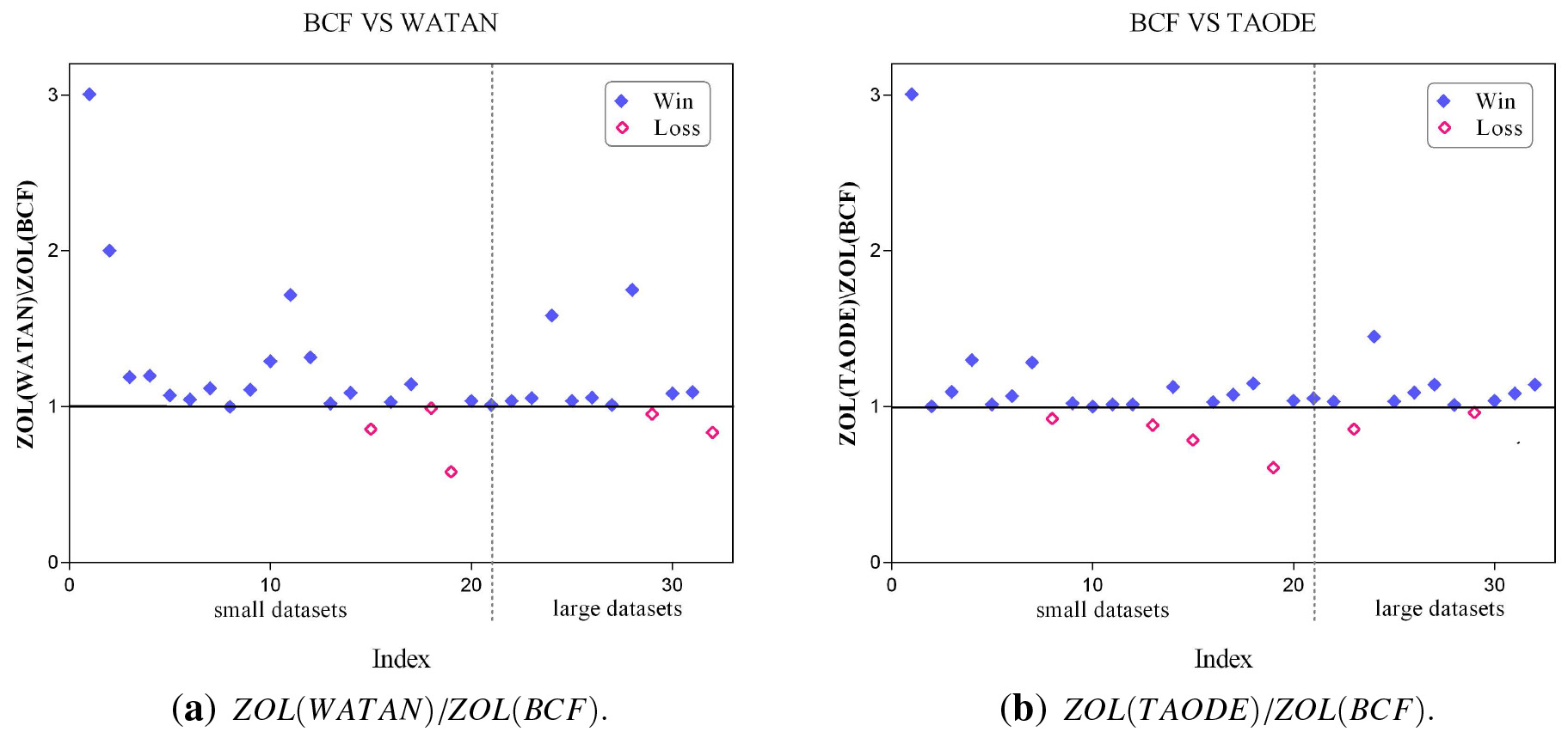
We compare the RMSE results for all of the above 6 state-of-the-art BNCs on 32 datasets to clarify their differences and present the W/D/L records in Table 5. The joint probability distribution can be factorized into
As shown in Table 5, ensemble learners perform better than single-model learner in terms of RMSE, e.g., WATAN beats CFWNB on 14 datasets and loses on 9. Thus the strict independence assumption of NB make the positive effect of weighting less significant. Weighted AODEs perform better than WATN in general, e.g., WAODE-MI beats WATN on 11 datasets and loses on 3. The topology diversity is explicable in terms of underlying independence assumptions of SPODE members, and the advantage of weighted AODEs can be attributed to the diversity and complementarity. BCF also embodies these characteristics in its learning procedure. It applies conditional entropy to measure directed causality and uses different root cause to learn different causal trees, thus achieving the trade-off between data fitting and causal reasoning. BCF demonstrates significant advantage over other learners, e.g., BCF respectively beats CFWNB, WATN and TAODE on 17, 11 and 15 datasets.
The scatter plot of RMSE for BCF and other two algorithms.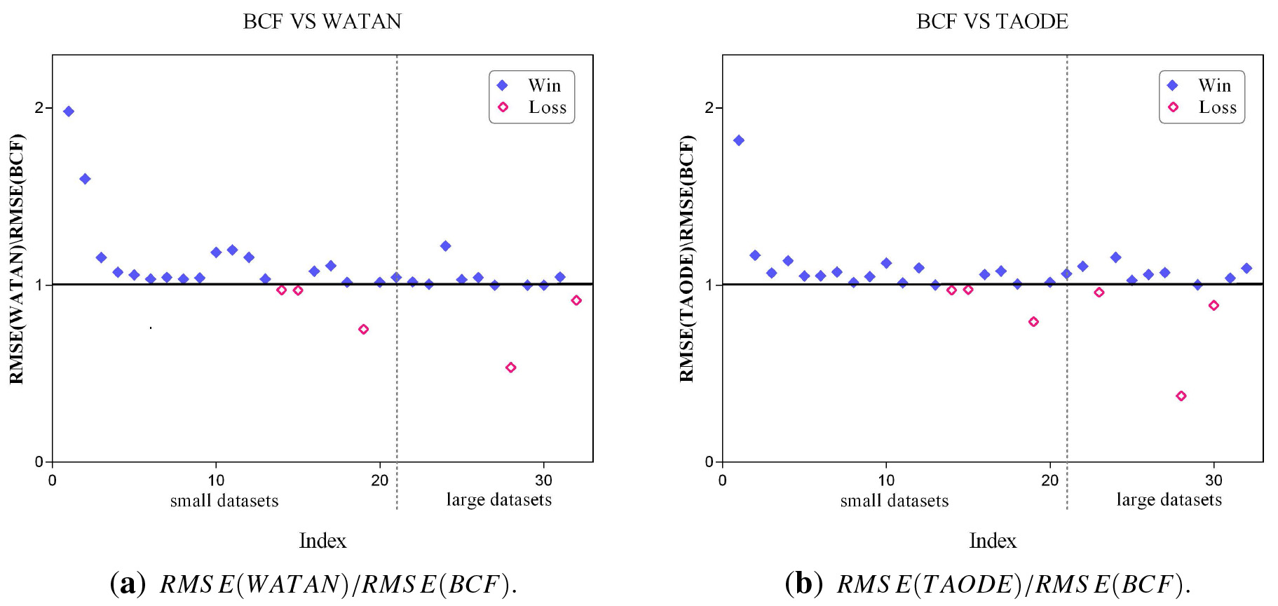
In order to give the results a more intuitionistic explanation, we present the scatter plot of RMSE for BCF and other two algorithms in Fig. 7, where the X-axis shows the index number of datasets and the Y-axis corresponds to the values of
Since
Win-Draw-Loss results of F1-Score on 32 datasets
Win-Draw-Loss results of F1-Score on 32 datasets
The W/D/L records summarizing the F1-Score of the state-of-the-art BNC algorithms are shown in Table 6, from which we can see that CFWNB performs better than weighted AODEs and WATAN in terms of F1-Score, e.g., CFWNB respectively beats WATN, IWAODE and TAODE on 10, 9 and 12 datasets. Weighted AODEs perform better in terms of F1-Score than WATAN. For example, TAODE beats WATAN on 5 datasets and loses on 2. The experimental results of IWAODE, WAODE-MI and TAODE are very similar, TAODE only outperforms IWAODE on 2 datasets. TAODE and WAODE-MI almost perform the same (30 draws). BCF performs the best among all of the above algorithms. When compared with single-model BNC, BCF performs better than CFWNB (12/9/7). When compared with ensemble BNCs, the advantages of BCF over WATAN, WAODE-MI and TAODE are also significant (13/18/1, 16/14/2 and 14/16/2, respectively). The results indicate that BCF can achieve significant improvements in terms of F1-Score.
Figure 8 shows the empirical time comparisons of the different out-of-core BNCs relative to BCF. All the experiments have been conducted on a desktop computer with an Intel(R) Core(TM) i5-8265U CPU @ 1.6 GHz, 64 bits and 8 G of memory. The algorithms described above are implemented using C
As shown in Fig. 8, the training procedures of IWAODE and TAODE are just the same as that of AODE, i.e., no structure learning and weighting are required. Thus they need the least time for training. During the testing phase, IWAODE and TAODE learn weights from each testing instance, and this instantiated weighting approach adjusts the weights flexibly but requires more time for testing. WAODE-MI needs to compute mutual information
BCF vs. SVM, LR and k-NN
W/D/L records of all compared algorithms in terms of zero-one loss, RMSE and F1-Score on 30 datasets
W/D/L records of all compared algorithms in terms of zero-one loss, RMSE and F1-Score on 30 datasets
Comparison of averaged training time and classification time for state-of-the-art BNCs on 32 datasets.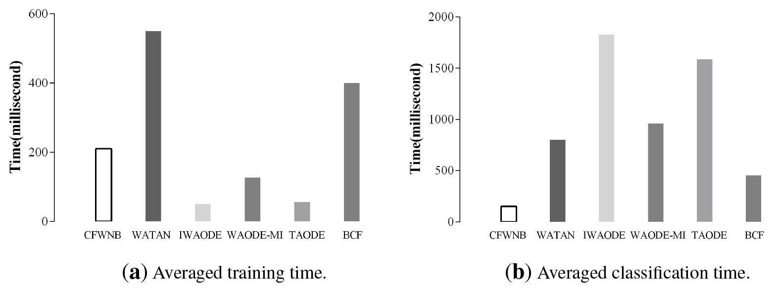
In this section, we compare BCF with SVM, LR and k-NN. The W/D/L records for BCF vs. LR, RF and k-NN in terms of zero-one loss, RMSE and F1-Score are given in Table 7. As we cannot obtain the results of SVM, LR and k-NN on the two datasets (labor and census-income), the comparison in this section only includes 30 datasets. From Table 7 we can see that, BCF performs better than SVM, LR and k-NN in terms of zero-one loss, e.g., BCF beats SVM on 23 datasets and loses on 6, and beats LR on 20 datasets and loses on 5. When compared with non-Bayesian learners in terms of RMSE, the advantages of BCF over SVM, LR and k-NN are also significant (25/2/3, 19/7/4 and 19/3/8, respectively). BCF also performs better than SVM, LR and k-NN in terms of F1-Score. For example, BCF beats SVM on 19 datasets and loses on 5, and beats k-NN on 15 datasets and loses on 7. For these non-Bayesian learners (SVM, LR and k-NN), the experiments with 30 datasets were performed on Weka (version 3.5.7), a widely used machine learning work-branch. Figure 9 displays the empirical time comparisons of the different non-Bayesian learners relative to BCF. During the training phase, SVM maps training instances to points in space so as to maximise the width of the gap between the two categories. Test instances are then mapped into that same space and predicted to belong to a category based on which side of the gap they fall. Thus SVM requires more time for training and testing in contrast to BCF. During the testing phase, k-NN needs to compute euclidean distance between a test instance and the specified training instances, thus k-NN needs a bit less time for training and more time for testing in contrast to SVM, LR and BCF. The goal of LR is to model the probability of a random variable being 0 or 1 given experimental data. During the training phase, LR uses optimization techniques such as gradient descent to maximize loss function. Therefore, learning of the LR is a very training time consuming but needs the least time for testing. In contrast, BCF considers more appropriate low-level heuristics, in addition to more iterations, during the heuristic search to facilitate more opportunity to undertake effective search.
Comparison of averaged training time and classification time for SVM, LR, k-NN and BNC on 30 datasets.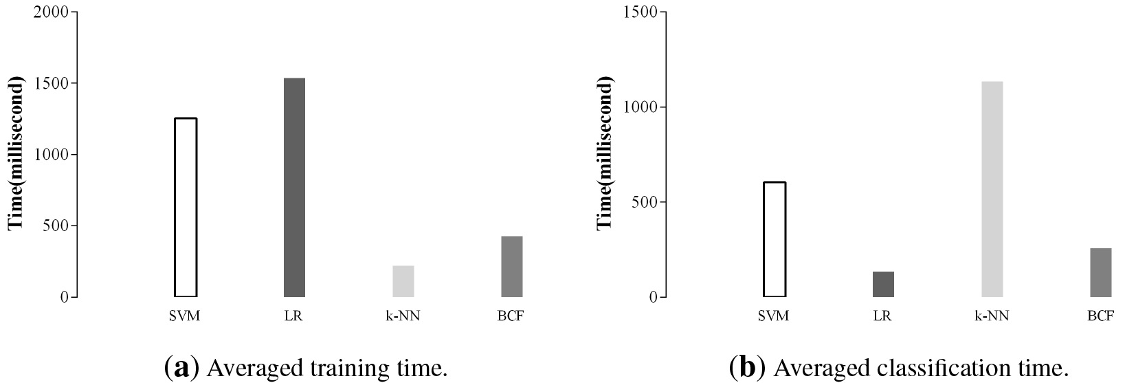
In this section, we compare the AUC results for all of the above 9 algorithms on 15 datasets with two classes in our experiments to clarify their differences and present the detailed results of AUC in Table 8. All 15 datasets are denoted with the symbol
Detailed results in terms of AUC on 15 datasets
Detailed results in terms of AUC on 15 datasets
The line chart of AUC comparisons for BNC and other four algorithms.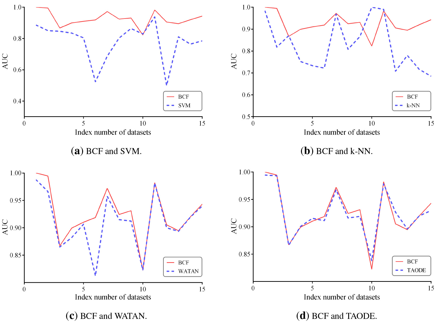
Average ranks of the algorithms
Average ranks of the algorithms
In this section, we perform the Friedman test followed by the Nemenyi test to explore the statistical significance of experimental results of these 9 algorithms on 30 datasets. The average ranks of the algorithms obtained by applying the Friedman test with respect to zero-one loss and RMSE are shown in Table 9. The Friedman statistic
The comparison results of Nemenyi test in terms of (a) zero-one loss and (b) RMSE.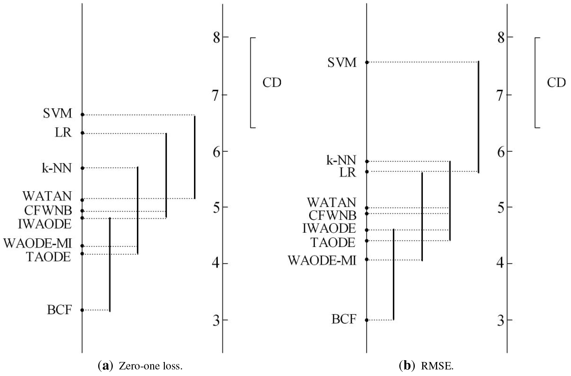
When the experimental results of zero-one loss are compared, from Fig. 11a we can see that BCF achieves the lowest mean zero-one loss rank (3.200) followed by TAODE (4.217), WAODE-MI (4.250) and IWAODE (4.733). Thus BCF enjoys significant zero-one loss advantage over CFWNB, WATAN, k-NN, LR and SVM. When RMSE is compared, from Fig. 11b we can see that BCF gets the first position in terms of zero-one loss, which is significantly different from CFWNB, WATAN, LR, k-NN and SVM, but there are no statistical differences between WAODE-MI, TAODE, IWAODE and BCF. These results illustrate the causal relationships or ensemble learning have an obvious positive effect on reducing the zero-one loss and RMSE of algorithm.
Our work has been primarily motivated by the intuitive understanding how one variable influences another in the network topology. Information-theoretic metrics, e.g., conditional mutual information
Footnotes
Acknowledgments
This work is supported by the National Key Research and Development Program of China (No. 2019YFC1804804) and the Scientific and Technological Developing Scheme of Jilin Province (No. 20200201281JC).
Appendix
Detailed results in terms of zero-one loss
Dataset
SVM
k-NN
LR
CFWNB
WATAN
IWAODE
WAODE-MI
TAODE
BCF
labor
Null
Null
Null
0.0701
0.0526
0.0526
0.0527
0.0526
0.0175
labor-negotiations
0.0702
0.1754
0.0702
0.1052
0.1053
0.0526
0.0526
0.0526
0.0526
lymphography
0.1824
0.1891
0.2162
0.1486
0.1689
0.1419
0.1554
0.1554
0.1419
iris
0.0333
0.0467
0.0400
0.0600
0.0800
0.0867
0.0867
0.0867
0.0667
autos
0.6537
0.2390
0.2878
0.1902
0.2146
0.2098
0.1951
0.1951
0.2000
sonar
0.3413
0.1346
0.2740
0.1586
0.2212
0.2260
0.2260
0.2260
0.2115
glass-id
0.2430
0.2103
0.3224
0.1728
0.2196
0.2196
0.2570
0.2523
0.1963
heart
0.4259
0.2444
0.2556
0.1703
0.1926
0.1704
0.1778
0.1778
0.1926
hungarian
0.3605
0.2313
0.1599
0.1598
0.1735
0.1599
0.1565
0.1599
0.1565
soybean-large
0.2573
0.0782
0.1531
0.0977
0.1010
0.0912
0.0814
0.0783
0.0782
dermatology
0.1694
0.0546
0.0301
0.0191
0.0328
0.0191
0.0192
0.0191
0.0191
cylinder-bands
0.2333
0.2556
0.2130
0.1981
0.2463
0.1926
0.1796
0.1880
0.1870
chess
0.1615
0.1208
0.1143
0.1379
0.0926
0.1034
0.0944
0.0799
0.0907
balance-scale
0.1024
0.1344
0.1040
0.2496
0.2736
0.2832
0.2816
0.2832
0.2512
soybean
0.1127
0.0878
0.0615
0.0614
0.0527
0.0542
0.0483
0.0483
0.0615
credit-a
0.4449
0.1884
0.1478
0.1333
0.1507
0.1391
0.1362
0.1507
0.1464
crx
0.1719
0.1678
0.1477
0.1304
0.1478
0.1319
0.1377
0.1391
0.1290
tic-tac-toe
0.1221
0.0125
0.0167
0.3100
0.2265
0.2662
0.2724
0.2630
0.2286
vowel
0.1495
0.0071
0.1818
0.3050
0.1263
0.1697
0.1949
0.1323
0.2172
contraceptive-mc
0.4515
0.5567
0.4881
0.4677
0.4895
0.4942
0.4922
0.4902
0.4718
mfeat-mor
0.6450
0.3450
0.3240
0.3060
0.2980
0.3120
0.3130
0.3105
0.2945
kr-vs-kp
0.0610
0.0372
0.0244
0.0644
0.0776
0.0826
0.0576
0.0773
0.0748
dis
0.0154
0.0170
0.0170
0.0156
0.0154
0.0127
0.0143
0.0125
0.0146
hypo
0.0740
0.0867
0.0339
0.0121
0.0130
0.0114
0.0101
0.0119
0.0082
sign
0.3273
0.3340
0.4063
0.3700
0.2752
0.2789
0.2768
0.2743
0.2653
magic
0.3412
0.1906
0.2089
0.2033
0.1674
0.1744
0.1762
0.1725
0.1581
adult
0.2416
0.2049
0.1484
0.1499
0.1380
0.1502
0.1445
0.1558
0.1363
shuttle
0.0166
0.0007
0.0315
0.0020
0.0014
0.0011
0.0009
0.0008
0.0008
connect-4
0.2242
0.1900
0.2423
0.2847
0.2354
0.2409
0.2406
0.2374
0.2468
waveform
0.0271
0.0404
0.0279
0.0198
0.0202
0.0181
0.0181
0.0189
0.0186
localization
0.4209
0.2226
0.5950
0.4936
0.3575
0.3593
0.3566
0.3544
0.3265
census-income
Null
Null
Null
0.1666
0.0636
0.0994
0.0883
0.0871
0.0762
Detailed results in terms of RMSE
Dataset
SVM
k-NN
LR
CFWNB
WATAN
IWAODE
WAODE-MI
TAODE
BCF
labor
Null
Null
Null
0.2545
0.2105
0.1649
0.1920
0.1931
0.1062
labor-negotiations
0.2649
0.4113
0.2438
0.2810
0.2778
0.1739
0.2057
0.2029
0.1736
lymphography
0.302
0.2759
0.3242
0.2419
0.2705
0.2304
0.2496
0.2501
0.2341
iris
0.1491
0.1747
0.1424
0.1500
0.1958
0.2024
0.2091
0.2077
0.1825
autos
0.4322
0.2568
0.2828
0.2099
0.2320
0.2317
0.2290
0.2306
0.2194
sonar
0.5842
0.365
0.5235
0.3409
0.4130
0.4246
0.4091
0.4202
0.3992
glass-id
0.4025
0.3716
0.3812
0.2952
0.3315
0.3237
0.3422
0.3409
0.3174
heart
0.6526
0.4924
0.3485
0.3429
0.3765
0.3548
0.3572
0.3696
0.3640
hungarian
0.6005
0.4791
0.3372
0.3384
0.3418
0.3450
0.3380
0.3443
0.3285
soybean-large
0.1646
0.0855
0.1248
0.0886
0.0902
0.0866
0.0860
0.0856
0.0761
dermatology
0.2376
0.1339
0.0975
0.0648
0.0850
0.0661
0.0688
0.0718
0.0709
cylinder-bands
0.483
0.5045
0.4465
0.4111
0.4277
0.3952
0.4016
0.4056
0.3696
chess
0.4019
0.2608
0.2771
0.3208
0.2594
0.2835
0.2603
0.2510
0.2509
balance-scale
0.2613
0.28
0.2092
0.3589
0.3203
0.3201
0.3203
0.3198
0.3291
soybean
0.1089
0.0879
0.0758
0.0723
0.0654
0.0697
0.0646
0.0657
0.0674
credit-a
0.667
0.4334
0.3329
0.3116
0.3407
0.3271
0.3236
0.3350
0.3159
crx
0.3142
0.3259
0.3415
0.3142
0.3415
0.3259
0.3219
0.3322
0.3077
tic-tac-toe
0.3495
0.2315
0.1289
0.4334
0.4023
0.3992
0.4085
0.3984
0.3961
vowel
0.1649
0.0358
0.1722
0.1982
0.1254
0.1463
0.1633
0.1324
0.1669
contraceptive-mc
0.5486
0.599
0.4384
0.4305
0.4392
0.4392
0.4385
0.4394
0.4324
mfeat-mor
0.3592
0.258
0.181
0.1943
0.1941
0.1979
0.1983
0.1980
0.1860
kr-vs-kp
0.247
0.1946
0.1474
0.2779
0.2358
0.2635
0.2343
0.2561
0.2315
dis
0.124
0.1302
0.1228
0.1130
0.1098
0.1058
0.1046
0.1047
0.1092
hypo
0.1923
0.2081
0.1147
0.0739
0.0723
0.0698
0.0647
0.0685
0.0592
sign
0.4671
0.2892
0.421
0.3929
0.3504
0.3516
0.3519
0.3487
0.3397
magic
0.5841
0.4366
0.3839
0.3709
0.3461
0.3534
0.3526
0.3519
0.3320
adult
0.4915
0.4526
0.3202
0.3150
0.3076
0.3250
0.3197
0.3297
0.3078
shuttle
0.0689
0.0137
0.0852
0.0270
0.0177
0.0159
0.0131
0.0124
0.0331
connect-4
0.3866
0.3069
0.3358
0.3632
0.3315
0.3359
0.3390
0.3339
0.3384
waveform
0.1345
0.1641
0.1158
0.1116
0.0951
0.0859
0.0860
0.0865
0.0977
localization
0.2766
0.2012
0.261
0.2402
0.2095
0.2093
0.2087
0.2081
0.2002
census-income
Null
Null
Null
0.3638
0.2168
0.2785
0.2604
0.2599
0.2373
Detailed results in terms of F1-Score
Dataset
SVM
k-NN
LR
CFWNB
WATAN
IWAODE
WAODEMI
TAODE
BCF
labor
null
null
null
0.9300
0.9429
0.9429
0.9429
0.9429
0.9810
labor-negotiations
0.9290
0.8260
0.9310
0.8930
0.8845
0.9429
0.9429
0.9429
0.9230
lymphography
0.7630
0.7530
0.7840
0.8510
0.5614
0.8897
0.6929
0.5720
0.8715
iris
0.9670
0.9530
0.9600
0.9470
0.9200
0.9133
0.9133
0.9133
0.9133
autos
0.7210
0.7640
0.7120
0.8100
0.8482
0.8590
0.5845
0.5838
0.8825
sonar
0.6200
0.8650
0.7260
0.8410
0.7778
0.7721
0.7721
0.7721
0.7818
glass-id
0.7470
0.7900
0.6790
0.8230
0.7863
0.7868
0.7519
0.7571
0.8089
heart
0.4480
0.7550
0.8430
0.8290
0.8035
0.8269
0.8190
0.8190
0.8639
hungarian
0.8010
0.7690
0.8390
0.8360
0.8082
0.8224
0.8257
0.8232
0.8207
soybean-large
0.8230
0.8321
0.8212
0.8020
0.8621
0.8800
0.9456
0.9468
0.9899
dermatology
0.8140
0.9450
0.9700
0.9970
0.9635
0.9795
0.9773
0.9773
0.9820
cylinder-bands
0.7670
0.7370
0.7830
0.9930
0.7310
0.7927
0.8091
0.8005
0.9270
chess
0.8100
0.9310
0.8860
0.8550
0.8713
0.8562
0.8698
0.8893
0.9794
balance-scale
0.8620
0.8420
0.9010
0.4823
0.5041
0.4974
0.4984
0.4974
0.3929
soybean
0.9230
0.9100
0.9390
0.9380
0.9632
0.9685
0.9748
0.9727
0.9649
credit-a
0.4770
0.8110
0.8530
0.8670
0.8470
0.8587
0.8614
0.8470
0.8527
crx
0.8033
0.8132
0.8233
0.8700
0.8502
0.8658
0.8599
0.8584
0.9662
tic-tac-toe
0.8710
0.9870
0.9830
0.6750
0.7330
0.6832
0.6724
0.6872
0.7188
vowel
0.8480
0.9930
0.8180
0.6960
0.8735
0.8302
0.8045
0.8679
0.9288
contraceptive-mc
0.5400
0.4430
0.5080
0.5310
0.4978
0.4957
0.4978
0.5006
0.6039
mfeat-mor
0.3710
0.6540
0.7350
0.6760
0.6994
0.6831
0.6814
0.6843
0.6986
kr-vs-kp
0.9390
0.9630
0.9760
0.9350
0.9223
0.9170
0.9421
0.9224
0.9258
dis
0.9780
0.9820
0.9760
0.9850
0.5818
0.7746
0.7553
0.7851
0.9613
hypo
0.7820
0.8923
0.9650
0.9880
0.7057
0.7161
0.7210
0.7140
0.8265
sign
0.6660
0.8660
0.5890
0.6260
0.7230
0.7195
0.7215
0.7241
0.7256
magic
0.5350
0.8070
0.7840
0.7800
0.8076
0.7887
0.7880
0.7913
0.9039
adult
0.6850
0.7950
0.8460
0.8530
0.8063
0.8062
0.8095
0.8011
0.9066
shuttle
0.9532
0.999
0.967
0.998
0.8294
0.8590
0.8010
0.8198
0.8496
connect-4
0.7320
0.7710
0.7170
0.6520
0.5170
0.5321
0.5377
0.5506
0.4984
waveform
0.9730
0.9600
0.9720
0.9800
0.9798
0.9819
0.9819
0.9818
0.9812
localization
0.7820
0.7750
0.7520
0.3523
0.3953
0.3677
0.3757
0.3813
0.8971
census-income
null
null
null
0.8720
0.7662
0.7175
0.7312
0.7306
0.7514
Detailed results of rank in terms of zero-one loss
Dataset
SVM
k-NN
LR
CFWNB
WATAN
IWAODE
WAODE-MI
TAODE
BCF
labor-negotiations
5.5
9.0
5.5
7.0
8.0
2.5
2.5
2.5
2.5
lymphography
7.0
8.0
9.0
3.0
6.0
1.5
4.5
4.5
1.5
iris
1.0
3.0
2.0
4.0
6.0
8.0
8.0
8.0
5.0
autos
9.0
7.0
8.0
1.0
6.0
5.0
2.5
2.5
4.0
sonar
9.0
1.0
8.0
2.0
4.0
6.0
6.0
6.0
3.0
glass-id
6.0
3.0
9.0
1.0
4.5
4.5
8.0
7.0
2.0
heart
9.0
7.0
8.0
1.0
5.5
2.0
3.5
3.5
5.5
hungarian
9.0
8.0
5.0
3.0
7.0
5.0
1.5
5.0
1.5
soybean-large
9.0
1.5
8.0
6.0
7.0
5.0
4.0
3.0
1.5
dermatology
9.0
8.0
6.0
2.5
7.0
2.5
5.0
2.5
2.5
cylinder-bands
7.0
9.0
6.0
5.0
8.0
4.0
1.0
3.0
2.0
chess
9.0
7.0
6.0
8.0
3.0
5.0
4.0
1.0
2.0
balance-scale
1.0
3.0
2.0
4.0
6.0
8.5
7.0
8.5
5.0
soybean
9.0
8.0
6.5
5.0
3.0
4.0
1.5
1.5
6.5
credit-a
9.0
8.0
5.0
1.0
6.5
3.0
2.0
6.5
4.0
crx
9.0
8.0
6.0
2.0
7.0
3.0
4.0
5.0
1.0
tic-tac-toe
3.0
1.0
2.0
9.0
4.0
7.0
8.0
6.0
5.0
vowel
4.0
1.0
6.0
9.0
2.0
5.0
7.0
3.0
8.0
contraceptive-mc
1.0
9.0
4.0
2.0
5.0
8.0
7.0
6.0
3.0
mfeat-mor
9.0
8.0
7.0
3.0
2.0
5.0
6.0
4.0
1.0
kr-vs-kp
4.0
2.0
1.0
5.0
8.0
9.0
3.0
7.0
6.0
dis
5.5
8.5
8.5
7.0
5.5
2.0
3.0
1.0
4.0
hypo
8.0
9.0
7.0
5.0
6.0
3.0
2.0
4.0
1.0
sign
6.0
7.0
9.0
8.0
3.0
5.0
4.0
2.0
1.0
magic
9.0
6.0
8.0
7.0
2.0
4.0
5.0
3.0
1.0
adult
9.0
8.0
4.0
5.0
2.0
6.0
3.0
7.0
1.0
shuttle
8.0
1.0
9.0
7.0
6.0
5.0
4.0
2.5
2.5
connect-4
2.0
1.0
7.0
9.0
3.0
6.0
5.0
4.0
8.0
waveform
7.0
9.0
8.0
5.0
6.0
1.5
1.5
4.0
3.0
localization
7.0
1.0
9.0
8.0
5.0
6.0
4.0
3.0
2.0
Average rank
6.667
5.667
6.317
4.817
5.133
4.733
4.250
4.217
3.200
Detailed results of rank in terms of RMSE
Dataset
SVM
KNN
LR
CFWNB
WATAN
IWAODE
WAODE-MI
TAODE
BCF
labor-negotiations
6.0
9.0
5.0
8.0
7.0
2.0
4.0
3.0
1.0
lymphography
8.0
7.0
9.0
3.0
6.0
1.0
4.0
5.0
2.0
iris
2.0
4.0
1.0
3.0
6.0
7.0
9.0
8.0
5.0
autos
9.0
7.0
8.0
1.0
6.0
5.0
3.0
4.0
2.0
sonar
9.0
2.0
8.0
1.0
5.0
7.0
4.0
6.0
3.0
glass-id
9.0
7.0
8.0
1.0
4.0
3.0
6.0
5.0
2.0
heart
9.0
8.0
2.0
1.0
7.0
3.0
4.0
6.0
5.0
hungarian
9.0
8.0
2.0
4.0
5.0
7.0
3.0
6.0
1.0
soybean-large
9.0
2.0
8.0
6.0
7.0
5.0
4.0
3.0
1.0
dermatology
9.0
8.0
7.0
1.0
6.0
2.0
3.0
5.0
4.0
cylinder-bands
8.0
9.0
7.0
5.0
6.0
2.0
3.0
4.0
1.0
chess
9.0
5.0
6.0
8.0
3.0
7.0
4.0
2.0
1.0
balance-scale
2.0
3.0
1.0
9.0
6.5
5.0
6.5
4.0
8.0
soybean
9.0
8.0
7.0
6.0
2.0
5.0
1.0
3.0
4.0
credit-a
9.0
8.0
5.0
1.0
7.0
4.0
3.0
6.0
2.0
crx
2.5
5.5
8.5
2.5
8.5
5.5
4.0
7.0
1.0
tic-tac-toe
3.0
2.0
1.0
9.0
7.0
6.0
8.0
5.0
4.0
vowel
6.0
1.0
8.0
9.0
2.0
4.0
5.0
3.0
7.0
contraceptive-mc
8.0
9.0
3.0
1.0
5.5
5.5
4.0
7.0
2.0
mfeat-mor
9.0
8.0
1.0
4.0
3.0
5.0
7.0
6.0
2.0
kr-vs-kp
6.0
2.0
1.0
9.0
5.0
8.0
4.0
7.0
3.0
dis
8.0
9.0
7.0
6.0
5.0
3.0
1.0
2.0
4.0
hypo
8.0
9.0
7.0
6.0
5.0
4.0
2.0
3.0
1.0
sign
9.0
1.0
8.0
7.0
4.0
5.0
6.0
3.0
2.0
magic
9.0
8.0
7.0
6.0
2.0
5.0
4.0
3.0
1.0
adult
9.0
8.0
5.0
3.0
1.0
6.0
4.0
7.0
2.0
shuttle
8.0
3.0
9.0
6.0
5.0
4.0
2.0
1.0
7.0
connect-4
9.0
1.0
4.0
8.0
2.0
5.0
7.0
3.0
6.0
waveform
8.0
9.0
7.0
6.0
4.0
1.0
2.0
3.0
5.0
localization
9.0
2.0
8.0
7.0
6.0
5.0
4.0
3.0
1.0
Average rank
7.583
5.750
5.617
4.917
4.950
4.567
4.019
4.433
3.000