Improving multi-label learning by modeling Local label and feature correlations

Abstract

Multi-label learning deals with the problem that each instance is associated with multiple labels simultaneously, and many methods have been proposed by modeling label correlations in a global way to improve the performance of multi-label learning. However, the local label correlations and the influence of feature correlations are not fully exploited for multi-label learning. In real applications, different examples may share different label correlations, and similarly, different feature correlations are also shared by different data subsets. In this paper, a method is proposed for multi-label learning by modeling local label correlations and local feature correlations. Specifically, the data set is first divided into several subsets by a clustering method. Then, the local label and feature correlations, and the multi-label classifiers are modeled based on each data subset respectively. In addition, a novel regularization is proposed to model the consistency between classifiers corresponding to different data subsets. Experimental results on twelve real-word multi-label data sets demonstrate the effectiveness of the proposed method.

Keywords

Multi-label learning local label correlations local feature correlations

1. Introduction

Multi-label learning can deal with objects with various semantic meanings, and it has been widely used in various application fields [1], such as, text categorization [2, 3, 4], image annotation [5, 6, 7], music emotion categorization [8, 9] and clinical data analysis [10, 11]. The target of multi-label learning is to use the given data to learn an effective classifier, which can predict a set of relevant category labels for new data instances.

Figure 1.

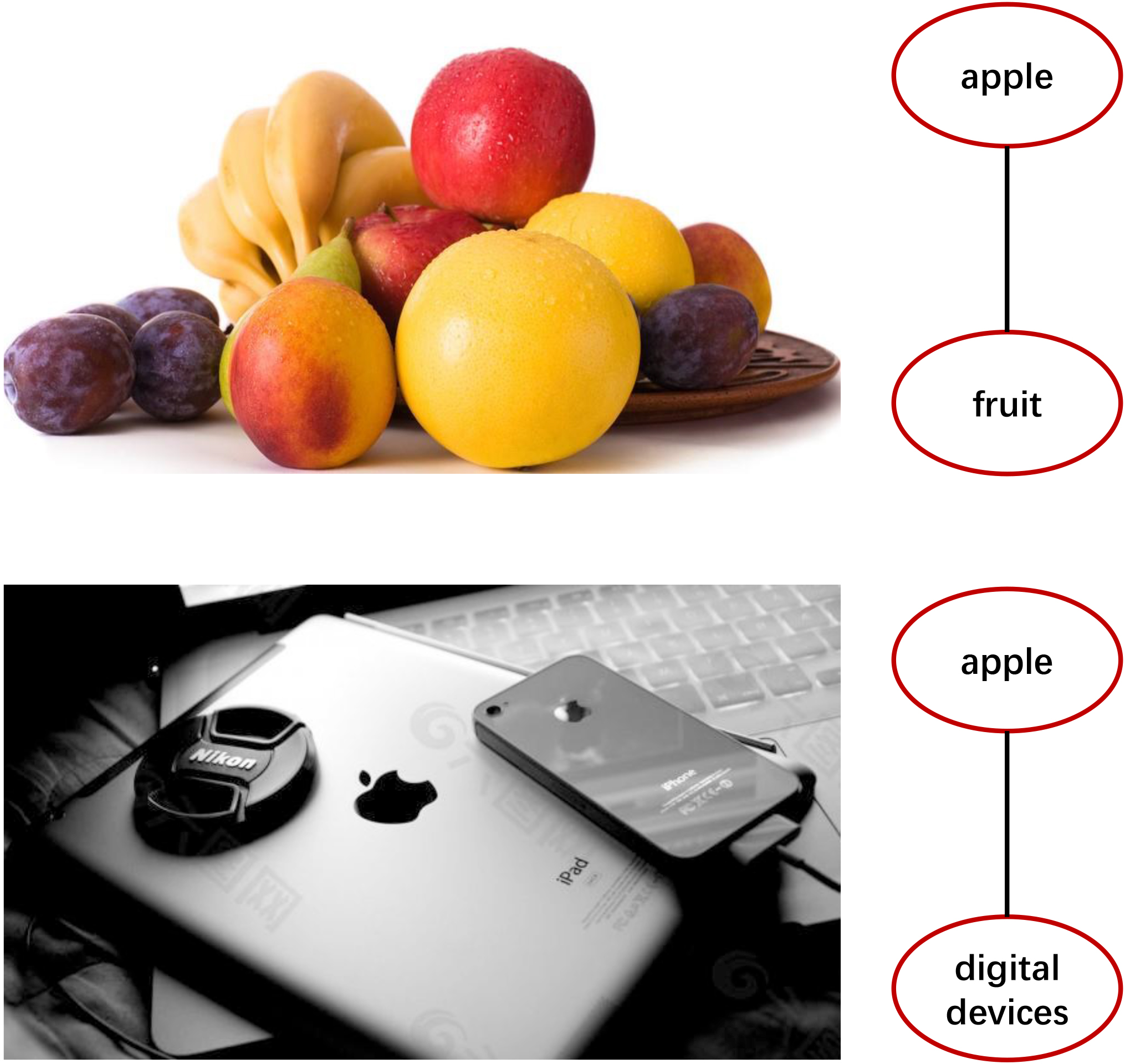
An example of local label correlation.

For multi-label learning, a simple and direct solution is to decompose the problem into a set of binary classification problems [12, 13], and each binary classification problem corresponds to a label. This approach may struggle to achieve good performance because it does not take into account the label correlations. Different to single-label learning, multi-label data involves complex correlations [1] between labels, i.e., the labels may correlated with each other. In other words, the information of a label can provide additional information for the labels related to it. To solve this problem, a large number of multi-label learning methods have been proposed to incorporate label correlations. However, most existing multi-label learning methods focus on global label correlations which are shared by all the instances [14, 15, 16, 17, 18, 19, 20, 21, 22]. In practical applications, label correlations may only be locally shared by different data subsets [23, 24, 25, 26, 27, 28]. For example, in Fig. 1, there is a picture of various fruits and a picture of digital devices. When only focusing on the pictures of fruit, label “apple” is related to “fruit”, and it is not related to “digital devices”. When only focusing on the pictures containing digital devices, label “apple” is related to “digital devices” not to “fruit”. This observation indicates that it is necessary to model label correlations for different data subsets respectively. Some methods [24, 25, 26] have been proposed to model local label correlations for multi-label learning, but they ignoring the relationship between features. On the other hand, in the environment of big data, the feature space of data sets becomes larger and larger, so feature redundancy may exist in the large feature space. Exploiting feature correlation can help to get rid of redundant features and obtain a more compact feature space, and further improve the performance of a model. Some methods [29, 30] introduce feature correlations into multi-label learning.Assuming that if two features are correlated, then their corresponding parameter vectors are also close. Similar to label correlation, feature correlation should also be modeled locally for different data subsets [31].

In this paper, a method is proposed to exploit Local Label and Feature Correlations for multi-label learning, namely LLFC. The local correlations of labels and features are integrated into a unified framework. Considering that the correlations corresponding to different data subsets are different, the classification models corresponding to each data subset are also different. Similar to CLMLC [32] and CBMLC [33], the data set is decomposed into several disjoint data groups, and then LLFC learns a classifier for each data group. But different from CLMLC and CBMLC, LLFC trains a classifier for each data group by modeling local label and feature correlations. The label correlations are used to constrain on the outputs of labels by assuming that if two labels are related then their corresponding outputs are similar. Besides, considering the relationship between different data clusters, if two data subsets are similar, their corresponding model parameters will be also similar, and then a new regularization term is proposed to control the similarity between different clusters by constraining the consistency of the models. In the testing stage, multiple classifiers are selected to predict the labels for the test data. The contributions of this paper are summarized as follows:

•

To the best of our knowledge, this paper is the first one to model the local correlation of labels and features into a unified framework for multi-label learning.

•

The consistency between different models corresponding to different data subsets is modeled.

•

Experimental results on twelve real-word multi-label data sets demonstrate the effectiveness of the proposed method.

The rest of this paper is organized as follows. Section 2 introduces some previous methods of multi-label learning, Section 3 describes the method LLFC in detail, Section 4 provides the experimental results and analyses. Finally, we conclude this paper in Section 5.

2. Related works

In multi-label learning, labels are usually correlated with each other, and modeling label correlations plays a crucial role in improvement of performance.

According to the order of correlations that the learning techniques have considered, existing methods are usually divided into three categories: first-order, second-order and higher-order strategies [1, 34]. The first-order strategy takes no account of the interaction between the labels and divides a multi-label learning problem into several independent single-label learning problems, and such as the representative algorithms BR [12], LIFT [35] and MLKNN [36]. The first-order strategy is simple and efficient, but it doesn’t consider the correlation between labels, which may be difficult to achieve good performance in most cases. To solve this problem,researchers set out to explore pairwise label correlations, known as second-order strategy, such as [14, 23, 37, 38, 39]. In fact, a label may depend on multiple labels simultaneously. The high-order strategy considers the interaction between multiple labels, such as [18, 40, 41, 42, 43, 44]. This strategy mines strong label correlations, but it may lead to a high computational complexity.

Besides, according to the scope of application of label correlations, existing methods are mainly divided into global and local strategies. For the global strategy, the label correlation is learned and exploited globally for the whole data. For example, ML-LRC [18] applies a kernel regularization to capture label correlations, and successfully captures global label correlations by using low rank structure on label correlation matrix. LSLC-ML [45] uses a manifold regularization to model positive and negative label correlations to recover missing labels for multi-label learning. These two methods only consider global label correlations,while in practical application, label correlations may not be globally applicable. Global label correlations may introduce irrelevant labels into the model. For the local strategy, label correlations are learned and exploited locally for different subsets of a data set. For example, ML-LOC [24] extends the original features by adding a code vector for each instance to exploit local label correlations. It divides the training data into several groups by a clustering method, and then generates prototypes of label vectors for each set. The code vector is composed of the similarities between the label vector of each instance and these archetypes. CLFS [25] divides the training data into several subsets by clustering, then it models local label correlations on each subset and constrains the correlations on outputs. GLOCAL [26] integrates global and local label correlations by label manifold regularization and constrains label correlations on outputs, which achieves good results. While these methods only focus on the local correlation of labels and ignore the relationship between features.

The information in the feature space is also very important for constructing multi-label learning models [15, 46]. For example, ML-LSS [46] utilizes local sample similarity for multi-label learning. It assumes that if the data samples are similar in a feature subset, their corresponding labels will also be similar. Although this method utilizes the information in the feature space, it only considers the correlation between instances and does not directly model the correlation between features. Exploiting feature correlations can help to remove the redundancy between features and get a more compact feature space. For example, MSSL [30] combines feature manifold learning and sparse regularization into a joint framework to study the problem of multi-label feature selection, and makes use of global feature correlations through feature manifolds. Similar to label correlation, the feature correlation may also be locally shared by different subsets of data examples. FSLCLC [31] explores local feature correlations on different subsets of examples, and tries to learn the potential relationship between features and labels. However, this method only model local feature correlations and Learn the same classifier for different data subsets. Through the analyses of previous studies, most of the existing multi-label learning methods only model the label correlations or feature correlations separately. To further improve the classification performance of multi-label learning, DRMFS [29] uses feature graph regularization and label graph regularization to preserve the geometric structure of feature manifolds and label manifolds respectively, which is the first time to integrate global feature correlations and label correlations into a unified framework. However, as discussed above, different subsets of data correspond to different label correlations and feature correlations, and exploiting global correlation of labels and features may bring unnecessary or even misleading constraints to the model.

To solve the mentioned problems, in this paper, we propose to construct the model by exploring the local correlation of labels and features simultaneously.

Figure 2.

The framework of the proposed method.

3. The proposed method

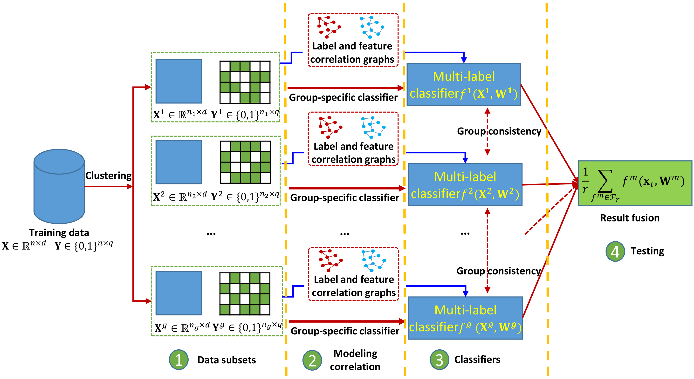
In this section, details of the proposed method LLFC are introduced, and the framework of it is shown in Fig. 2. The framework diagram is mainly composed of four parts, which are divided by the orange dotted line in the figure. As shown in the figure, step 1 is to divide the train data into multiple disjoint data subsets by clustering. $\{\textbf{X}^{1},\textbf{X}^{2},\ldots,\textbf{X}^{g}\}$ and $\{\textbf{Y}^{1},\textbf{Y}^{2},\ldots,\textbf{Y}^{g}\}$ are data subsets and label subsets respectively. The blue rectangles represent the data matrices corresponding to all the data subsets $\{\textbf{X}^{i}\}_{i=1}^{g}$ , and the rectangles with white and green color indicate the corresponding label matrices of $\{\textbf{Y}^{i}\}_{i=1}^{g}$ . The white color indicates that the element value of the matrix is 0, that means the label is not included, and the green color indicates that the element value in the matrix is 1, which means that the label is included. In step 2, local label and feature correlations are modeled by manifold regularization to construct the group-specific multi-label classifiers for each data subset. In step 3, the consistency between different group-specific classifiers is modeled. Finally, step 4 is the test stage, and $r$ nearest classification models are selected to predict possible labels for the test data.

3.1 Data clustering

In multi-label learning, assuming $\textbf{X}\in\mathbb{R}^{d}$ is a $d$ dimensional feature space and $y=\{y_{1},y_{2},\ldots,y_{q}\}$ represents a label set with $q$ class labels. $\mathcal{D}=\{(\textbf{x}_{i},\textbf{y}_{i})|1\leqslant i\leqslant n\}$ is a train data set with $n$ instances. $\textbf{Y}=[\textbf{y}_{1},\textbf{y}_{2},\ldots,\textbf{y}_{n}]^{T}\in\{0,1\}% ^{n\times q}$ is the label matrix, and $\textbf{y}_{i}=[y_{i1},y_{i2},\ldots,y_{iq}]\in\mathbb{R}^{1\times q}$ is a binary label vector corresponding to $\textbf{x}_{i}$ $(1\leqslant i\leqslant n)$ , where $y_{ij}=1$ $(1\leqslant j\leqslant n)$ represents $\textbf{x}_{i}$ belongs to $y_{j}$ , otherwise $y_{ij}=0$ .

To model the local label and feature correlations, similar to previous work [25, 26, 31], the data set is firstly divided into $g$ subsets by clustering. Then, the feature matrices $\{\textbf{X}^{1},\textbf{X}^{2},\ldots,\textbf{X}^{g}\}$ and label matrices $\{\textbf{Y}^{1},\textbf{Y}^{2},\ldots,\textbf{Y}^{g}\}$ for the subsets can be obtained, where $\textbf{X}^{m}\in\mathbb{R}^{n_{m}\times d}$ has $n_{m}$ instances, and $\textbf{Y}^{m}\in\mathbb{R}^{n_{m}\times q}$ is the label subset of Y corresponding to $\textbf{X}^{m}$ $(1\leqslant m\leqslant g)$ . After clustering, the cluster centers $\textbf{C}\in\mathbb{R}^{g\times d}$ for each data subset can be obtained, where $\textbf{c}_{m}=[c_{m}^{1},c_{m}^{2},\ldots,c_{m}^{d}]\in\mathbb{R}^{1\times d}$ is the $m$ -th row of C and represents the clustering center vector of the $m$ -th subset.

3.2 Model construction

For each data subset, a multi-label classifier can be constructed. Specifically, a classifier $f^{m}$ is learned for the $m$ -th subset based on $\textbf{X}^{m}$ and $\textbf{Y}^{m}$ . In this paper, the linear classifier is adopted, and ${f}^{m}(\cdot)$ is defined as

$\displaystyle{f}^{m}(\textbf{x}_{i}^{m})=\textbf{x}_{i}^{m}\textbf{W}^{m}+% \textbf{b}^{m},$ (1)

where $\textbf{x}_{i}^{m}\in\mathbb{R}^{1\times d}$ indicates the $i$ -th instance in the $m$ -th data subset, and $\textbf{W}^{m}\in\mathbb{R}^{d\times q}$ is the model coefficient of the linear model ${f}^{m}(\cdot)$ . $\textbf{b}^{m}$ denotes the bias, and it can be absorbed into $\textbf{W}^{m}$ by adding the constant value 1 to each data instance $\textbf{x}_{i}^{m}$ as an additional feature.

In this paper, an independent model coefficient is learned for each subset through the least squares loss function with F-norm constraints. Consequently, the basic model of LLFC can be constructed as follows

$\displaystyle\min_{\{{\textbf{W}}^{m}\}_{m=1}^{g}}\frac{1}{2}\sum\limits_{m=1}% ^{g}\left(||{\textbf{X}}^{m}{\textbf{W}}^{m}-{\textbf{Y}}^{m}||_{F}^{2}+% \lambda_{3}||{\textbf{W}}^{m}||_{F}^{2}\right),$ (2)

where $\lambda_{3}$ is the non-negative model parameter, $\{\textbf{W}^{1},\textbf{W}^{2},\ldots,\textbf{W}^{g}\}$ are the model coefficients, $\textbf{W}^{m}\in\mathbb{R}^{d\times q}$ is the weight coefficient matrix of the $m$ -th model $f^{m}$ constructed based the $m$ -th data subset $\textbf{X}^{m}\in\mathbb{R}^{n_{m}\times d}$ .

3.3 Learning local label correlations

In multi-label learning, the correlation between different labels provides additional information for multi-label learning, which is very helpful to improve the performance of classifier. Previous approaches usually exploit label correlation in a global way, and assume that label correlations are shared by all instances [14, 15, 16, 17, 18, 19, 20, 21, 22]. However, in some real applications, label correlations are locally applicable. In this paper, explore local label correlation for each model $f^{m}$ by adding a manifold regularization to constrain the correlations on the outputs of labels in each data subset.

Motivated by previous work CLFS [25] and GLOCAL [26], the training data is divided into $g$ different subsets, the local label correlation matrices are calculated according to the corresponding label subset of each data subset. Let $\textbf{B}^{m}\in\mathbb{R}^{q\times q}$ be label correlation matrix which corresponds to the $m$ -th label subset $\textbf{Y}^{m}$ . $b_{ij}^{m}$ is the element of $\textbf{B}^{m}$ in the $i$ -th row and $j$ -th column, and it represents the correlation between the $i$ -th and $j$ -th label of $\textbf{Y}^{m}$ . By the cosine similarity, $b_{ij}^{m}$ can be calculated as follows

$\displaystyle b_{ij}^{m}=\sum\limits_{h=1}^{n_{m}}y_{hi}^{m}y_{hj}^{m}\left/% \left(\sqrt[2]{\sum\limits_{h=1}^{n_{m}}{y_{hi}^{m}}^{2}}\sqrt[2]{\sum\limits_% {h=1}^{n_{m}}{y_{hj}^{m}}^{2}}\right),\right.$ (3)

where $y_{hi}^{m}$ indicates element of $\textbf{Y}^{m}$ in the $h$ -th row and $i$ -th column.

After obtaining the $g$ local label correlation matrices, it can be used to model local label correlations for the models $f^{m}$ $(1\leqslant m\leqslant g)$ . Specifically, for each data subset, assuming that if two labels are highly correlated, their corresponding output should be more similar, i.e. if $y_{i}$ and $y_{j}$ are highly correlated in the $m$ -th subset, the outputs of $f_{i}^{m}$ and $f_{j}^{m}$ should be similar, and vice versa. $f_{i}^{m}$ and $f_{j}^{m}$ are the i-th column and j-th column of $\textbf{F}^{m}$ , and $\textbf{F}^{m}=\textbf{X}^{m}\textbf{W}^{m}\in\mathbb{R}^{n_{m}\times q}$ . Consequently, the regularization term for modeling local label correlation for each model $f^{m}$ $(1\leqslant m\leqslant g)$ can be defined as

$\displaystyle\frac{1}{4}\sum\limits_{m=1}^{g}\left(\sum\limits_{i=1}^{q}\sum% \limits_{j=1}^{q}{b_{ij}^{m}}||{\textbf{X}}^{m}{\textbf{w}}_{i}^{m}-{\textbf{X% }}^{m}{\textbf{w}}_{j}^{m}||^{2}_{2}\right)$ $\displaystyle=\frac{1}{2}\sum\limits_{m=1}^{g}\textbf{tr}({\textbf{X}}^{m}{% \textbf{W}}^{m}{\textbf{L}}_{m}^{Y}({\textbf{X}}^{m}{\textbf{W}}^{m})^{T})$ (4) $\displaystyle=\frac{1}{2}\sum\limits_{m=1}^{g}\textbf{tr}({\textbf{F}}^{m}{% \textbf{L}}_{m}^{Y}{{\textbf{F}}^{m}}^{T}),$

where $\textbf{L}_{m}^{Y}=\textbf{D}_{m}^{Y}-\textbf{B}^{m}$ is the Laplacian matrix of the label correlation matrix $\textbf{B}^{m}$ , $\textbf{D}_{m}^{Y}$ is a diagonal matrix with diagonal elements $D_{ii}^{Y}=\sum_{j=1}^{q}b_{ij}^{m}$ , and $\textbf{w}_{i}^{m}$ and $\textbf{w}_{j}^{m}$ are the $i$ -th and $j$ -th columns of $\textbf{W}^{m}$ respectively. By combining the local label correlations, the objective Eq. (2) can be rewritten as follow

where $\lambda_{1}$ is a non-negative weight coefficient.

3.4 Learning local feature correlations

In multi-label learning, there is not only correlation between labels, but also correlation between features, and exploiting feature correlations can help to remove redundant features and obtain a more compact feature space. Similar to local label correlations, different instances may correspond to different feature correlations. Therefore, in order to get $g$ improved coefficient matrices, this paper introduces the manifold regularization based on local feature correlations for multi-label learning. For each data subset, the cosine similarity is adopted to calculate the feature correlations. Let $\textbf{S}^{m}\in\mathbb{R}^{d\times d}$ be the feature correlation matrix which corresponds to the m-th data subset $\textbf{X}^{m}$ , and element $s_{lk}^{m}$ is defined as

$\displaystyle s_{lk}^{m}=\sum\limits_{h=1}^{n_{m}}x_{hl}^{m}x_{hk}^{m}\left/% \left(\sqrt[2]{\sum\limits_{h=1}^{n_{m}}{x_{hl}^{m}}^{2}}\sqrt[2]{\sum\limits_% {h=1}^{n_{m}}{x_{hk}^{m}}^{2}}\right),\right.$ (6)

where $s_{lk}^{m}$ is the $l$ -th row and $k$ -th column element of $\textbf{S}^{m}$ and represents the similarity between the $l$ -th and $k$ -th features in $\textbf{X}^{m}$ . $x_{hl}^{m}$ and $x_{hk}^{m}$ represent the $h$ -th row and $l$ -th column element and the $h$ -th row and $k$ -th column element of $\textbf{X}^{m}$ respectively.

For each data subset, supposing that if two features in $\textbf{X}^{m}$ are similar, the model coefficients corresponding to these two features are similar too, i.e. if $\textbf{x}_{l}^{m}$ and $\textbf{x}_{k}^{m}$ are more similar, then their weight vectors $\textbf{w}_{l}^{m}$ and $\textbf{w}_{k}^{m}$ should be similar as well, where $\textbf{w}_{l}^{m}$ and $\textbf{w}_{k}^{m}$ are the $l$ -th and $k$ -th rows of $\textbf{W}^{m}$ respectively, and $\textbf{x}_{l}^{m}$ and $\textbf{x}_{k}^{m}$ are the $l$ -th and $k$ -th columns of $\textbf{X}^{m}$ respectively. Similar to the construction of local label correlation, the following regularization term is defined to model local feature correlation

$\displaystyle\frac{1}{4}\sum\limits_{m=1}^{g}\left(\sum\limits_{l=1}^{d}\sum% \limits_{k=1}^{d}{s_{lk}^{m}}||{\textbf{w}}_{l}^{m}-{\textbf{w}}_{k}^{m}||_{2}% ^{2}\right)$ (7) $\displaystyle=\frac{1}{2}\sum\limits_{m=1}^{g}\textbf{tr}({{\textbf{W}}^{m}}^{% T}{\textbf{L}}_{m}^{X}{\textbf{W}}^{m}),$

where $\textbf{L}_{m}^{X}=\textbf{D}_{m}^{X}-\textbf{S}^{m}$ is the Laplacian matrix of $\textbf{S}^{m}$ , $\textbf{D}_{m}^{X}$ is a diagonal matrix with $D_{ll}^{X}=\sum_{k=1}^{d}s_{lk}^{m}$ . By combing feature correlations, the objective Eq. (5) can be reformulated as follows

$\displaystyle\min_{\{{\textbf{W}}^{m}\}_{m=1}^{g}}\frac{1}{2}\sum\limits_{m=1}% ^{g}(||{\textbf{X}}^{m}{\textbf{W}}^{m}-{\textbf{Y}}^{m}||_{F}^{2}+\lambda_{1}% \textbf{tr}({\textbf{F}}^{m}{\textbf{L}}_{m}^{Y}{{\textbf{F}}^{m}}^{T})+% \lambda_{2}\textbf{tr}({{\textbf{W}}^{m}}^{T}{\textbf{L}}_{m}^{X}{\textbf{W}}^% {m})+\lambda_{3}||{\textbf{W}}^{m}||_{F}^{2}),$ (8)

where $\lambda_{2}$ is a non-negative weight parameter.

3.5 Exploring the consistency between models

In this paper, the data set is divided into $g$ groups, and construct a model $f^{m}(1\leqslant m\leqslant g)$ for each each of them. Considering that the data subsets come from the same data distribution, the models for different subsets should be consistent to some extent. Therefore, we try to model the consistency between different models for the data groups. Specifically, if two data subsets are similar, their corresponding models will also be similar, i.e., if $\textbf{X}^{i}$ and $\textbf{X}^{j}$ are similar, $\textbf{W}^{i}$ and $\textbf{W}^{j}$ will be similar as well, where $\textbf{X}^{i}$ and $\textbf{X}^{j}$ are $i$ -th and $j$ -th data subsets, $\textbf{W}^{i}$ and $\textbf{W}^{j}$ are their corresponding model coefficients. Consequently, the following regularization term is defined to model the consistency between different models

$\displaystyle\frac{1}{2}\sum\limits_{m,j=1}^{g}a_{mj}||{\textbf{W}}^{m}-{% \textbf{W}}^{j}||_{F}^{2},$ (9)

where $a_{mj}$ represents similarity between the $m$ -th and $j$ -th data subsets, and $\textbf{A}=[a_{mj}]\in\mathbb{R}^{g\times g}$ . It can be obtained by calculating the similarity between the clustering center vectors of data subsets according to the following formulation

$\displaystyle a_{mj}=\sum\limits_{h=1}^{d}c_{mh}c_{jh}\left/\left(\sqrt[2]{% \sum\limits_{h=1}^{d}c_{mh}^{2}}\sqrt[2]{\sum\limits_{h=1}^{d}c_{jh}^{2}}% \right),\right.$ (10)

where $c_{mh}$ represents the $m$ -th row and $h$ -th column element and $c_{jh}$ represents the $j$ -th row and $h$ -th column element of C.

Finally, the final objective function of our proposed method LLFC can be defined as follows

$\displaystyle\min_{\{{\textbf{W}}^{m}\}_{m=1}^{g}}\frac{1}{2}\sum\limits_{m=1}% ^{g}(||{\textbf{X}}^{m}{\textbf{W}}^{m}-{\textbf{Y}}^{m}||_{F}^{2}+\lambda_{1}% \textbf{tr}({\textbf{F}}^{m}{\textbf{L}}_{m}^{Y}{{\textbf{F}}^{m}}^{T})+% \lambda_{2}\textbf{tr}({{\bf{W}}^{m}}^{T}{\bf{L}}_{m}^{X}{\bf{W}}^{m})+\lambda% _{3}||{\textbf{W}}^{m}||_{F}^{2})+\frac{\lambda_{4}}{2}\sum\limits_{m,j=1}^{g}% a_{mj}||{\textbf{W}}^{m}-{\textbf{W}}^{j}||_{F}^{2}$ (11)

where $\lambda_{4}$ is a non-negative model parameter.

3.6 Optimization

The objective Eq. (11) is convex and smooth, and the gradient descent method is used to optimize the solution. From the objective function, it need to solve the $g$ model coefficients $\{\textbf{W}^{1},\textbf{W}^{2},\ldots,\textbf{W}^{g}\}$ and adopt the alternating optimization strategy.

When updating the model coefficient $\textbf{W}^{m}$ for the $m$ -th group, the other model coefficients are fixed, and the problem Eq. (11) is simplified as follows

$\displaystyle\min\limits_{{\textbf{W}}^{m}}\frac{1}{2}(||{\textbf{X}}^{m}{% \textbf{W}}^{m}-{\textbf{Y}}^{m}||_{F}^{2}+\lambda_{1}\textbf{tr}({\textbf{F}}% ^{m}{\textbf{L}}_{m}^{Y}{{\textbf{F}}^{m}}^{T})+\lambda_{2}\textbf{tr}({{% \textbf{W}}^{m}}^{T}{\textbf{L}}_{m}^{X}{\textbf{W}}^{m})+\lambda_{3}||{\bf{W}% }^{m}||_{F}^{2})+\frac{\lambda_{4}}{2}\sum\limits_{j=1}^{g}a_{mj}||{\bf{W}}^{m% }-{\bf{W}}^{j}||_{F}^{2}$ (12)

As a result, the gradient w.r.t $\textbf{W}^{m}$ can be calculated as follows,

$\displaystyle\nabla_{{\textbf{W}}^{m}}={{\textbf{X}}^{m}}^{T}{\textbf{X}}^{m}{% \textbf{W}}^{m}-{{\textbf{X}}^{m}}^{T}{\textbf{Y}}^{m}+\lambda_{1}{{\textbf{X}% }^{m}}^{T}{\textbf{X}}^{m}{\textbf{W}}^{m}{\textbf{L}}_{m}^{Y}+\lambda_{2}{% \textbf{L}}_{m}^{X}{\textbf{W}}^{m}+\lambda_{3}\textbf{W}^{m}+\lambda_{4}\sum% \limits_{j=1}^{g}a_{mj}(\textbf{W}^{m}-{\textbf{W}}^{j})$ (13)

Then, $\textbf{W}^{m}$ can be updated by

$\displaystyle{{\textbf{W}}^{m}}_{t+1}\leftarrow{{\textbf{W}}^{m}}_{t}-\eta% \nabla_{{\textbf{W}}^{m}},$ (14)

where $\eta$ is a step size for $\textbf{W}^{m}$ , it is a small positive number. In this paper, we use an automatic step adjustment method [47] to set the value of $\eta$ .

[t]Optimization of LLFCTraining data: $\textbf{X}\in\mathbb{R}^{n\times d}$ , label matrix: $\textbf{Y}\in\mathbb{R}^{n\times q}$ , and the weighting parameters $\lambda_{1}$ , $\lambda_{2}$ , $\lambda_{3}$ , $\lambda_{4}$ , $\rho$ , and $g$ ; Model Coefficients: $\{\textbf{W}^{1},\ldots,\textbf{W}^{g}\}$ ;

Getting $\{\textbf{X}^{1},\ldots,\textbf{X}^{g}\}$ and $\{\textbf{Y}^{1},\ldots,\textbf{Y}^{g}\}$ through K-means clustering on X; Calculating A;

$m=1$ to $g$ Calculating $\textbf{L}_{m}^{Y}$ and $\textbf{L}_{m}^{X}$ ;

Initialization: $\textbf{W}^{m}\leftarrow{\textbf{X}^{m}}^{T}\textbf{Y}^{m}/({\textbf{X}^{m}}^{% T}\textbf{X}^{m}+\rho I)$ ; $t\leftarrow 1$ ;

converge $m=1$ to $g$ Fix $\textbf{W}^{1},\ldots,\textbf{W}^{m-1},{\textbf{W}^{m+1},\ldots,\textbf{W}}^{g}$ and update ${\textbf{W}^{m}}$ by Eq.(14); $t\leftarrow t+1$ ; return $\{\textbf{W}^{1},\ldots,\textbf{W}^{g}\}$ ;

3.7 Prediction

In Algorithm 3.6, the overall optimization steps of LLFC are summarized . After obtaining the model coefficients corresponding to each data subsets, the subsequent prediction can be made. Given a test instance $\textbf{x}_{t}\in\mathbb{R}^{1\times d}$ , the prediction of the LLFC algorithm can be done in two steps:1) find the $r$ nearest data subsets for the test instance; 2) combine the predictions from the models corresponding to the $r$ nearest data subsets.

First, the Euclidean distances between the test instance $\textbf{x}_{t}$ and the center vectors of $g$ data subsets are calculated to find the $r$ nearest data subsets. Then, the corresponding models $\mathcal{F}_{r}$ for the $r$ nearest data subsets are obtained. Finally, $r$ models are used to predict the labels for $\textbf{x}_{t}$ respectively, and then the average of the predicted results is taken as the final prediction result of $\textbf{x}_{t}$ .

$\displaystyle\textbf{z}_{t}=\frac{1}{r}\sum_{f^{m}\in\mathcal{F}_{r}}f^{m}({% \textbf{x}}_{t},{\textbf{W}}^{m})$ (15)

where $\textbf{z}_{t}\in\mathbb{R}^{1\times q}$ is the real label confidence vector of the test data $\textbf{x}_{t}$ , and a binary label vector $\textbf{y}_{t}\in\{0,1\}^{1\times q}$ corresponding to $\textbf{x}_{t}$ can be obtained based on a threshold value.

3.8 Time complexity

According to Algorithm 3.6, we can see that the time complexity of the algorithm is mainly controlled by the steps 6–10, where the model coefficients corresponding to each group-specific classifier should be calculated. For each group-specific classifier, the total time complexity is $\mathcal{O}(tg(d^{2}n_{m}+d^{2}q+dqn_{m}+dq^{2}))$ , where $n_{m}$ is the number of instances of the $m$ -th data subset. Therefore, the total time complexity is $\mathcal{O}(t(d^{2}n+d^{2}qg+dqn+gdq^{2}))$ , where $n$ is the total number of instances, $d$ is the number of features, $t$ is the number of iterations, $q$ is the number of labels and $g$ is the number of groups.

4. Experiment

4.1 Experimental setup

4.1.1 Data sets

In this paper, we perform the experimental analysis on twelve commonly used real multi-label data sets to verify the effectiveness of the proposed method. These data sets can be downloaded from Mulan,1

¹
http://mulan.sourceforge.net/datasets.html.

Lamda,2

http://lamda.nju.edu.cn/Data.ashx#data.

and Meka,3

http://meka.sourceforge.net.

and details are summarized in Table 1. For each data set, “

\#

Instance” indicates the number of instances, “

\#

Feature” denotes the number of features, “

\#

Label” represents the number of labels, and “

\#

Card” denotes the average number of labels per instance.

Table 1

Characteristics of the experimental data sets

ID	Dataset	#Instance	#Feature	#Label	Card
1	yeast	2417	103	14	4.24
2	arts	5000	462	26	1.64
3	reference	5000	793	33	1.17
4	corel5k	5000	499	374	3.52
5	rcv1subset1	6000	944	101	2.88
6	rcv2subset2	6000	944	101	2.63
7	rcv2subset3	6000	944	101	2.63
8	Corel16k001	13766	500	153	2.86
9	Corel16k002	13761	500	164	2.88
10	Stackex ${\_}$ cs	9270	635	274	2.65
11	Stackex ${\_}$ cooking	10491	577	400	2.23
12	Stackex ${\_}$ chess	1675	585	227	2.41

4.1.2 Comparing algorithms

In the experiment, we compared the proposed method with six existing multi-label learning methods. The optimal parameters for all of the algorithms are determined by a 5-fold cross validation. The detailed settings are summarized as follows:

1.
MLKNN[36]: This method is a lazy multi-label learning method, and does not consider the correlation between labels. The value range of parameter $k$ is $\{4,6,\ldots,20\}$ .
2.
CLMLC[32]: This method is a local multi-label classification method based on Scalable clustering, and it learns a model for each subsets by low dimensional clustering. The value ranges of parameters $d, k$ and $n$ are $\min\{q,30\}$ , $\{10,20,\ldots,200\}$ and $\{2,4,\ldots,20\}$ .
3.
ML-LSS[46]: It is a multi-label learning method with local similarity of samples. It assumes that if the feature subsets between samples are similar, the output of corresponding labels should also be similar. The value of parameters $\lambda_{1}$ and $\lambda_{2}$ are searched in $\{{2}^{-5},2^{-4},\ldots,2^{6}\}$ .
4.
LSF-CI[15]: It proposes to learn the label specific features of each label and takes into account the global label correlations in the label space and the instance correlations in the feature space. The value range of parameters $\alpha$ , $\beta$ , $\gamma$ is $\{{2}^{-10},2^{-9},\ldots,2^{10}\}$ .
5.
GLOCAL[26]: In this method, the global and local label correlations is obtained by the label manifolds to learn the full label and missing label. In this experiment, we use the full label method as the comparison method. The value of parameter $\lambda$ is $1$ , the value range of parameters $\lambda_{1}$ to $\lambda_{5}$ is $\{{10}^{-5},{10}^{-4},\ldots,{10}^{1}\}$ and parameters $k$ and $g$ are searched in among $\{0.1q,0.2q,\ldots,0.6q\}$ and $\{5,10,15,20\}$ respectively.
6.
JFSC[19]: The method is based on global label correlations for feature selection and multi-label learning. The value range of parameters $\alpha$ , $\beta$ and $\gamma$ is $\{{4}^{-5},4^{-4},\ldots,4^{5}\}$ and the value range of $\rho$ is $\{0.1,1,10\}$ .
7.
LLFC: The proposed method. The value range of parameters $\lambda_{1}$ and $\lambda_{2}$ is $\{{10}^{-5},{10}^{-4},\ldots,{10}^{1}\}$ and parameters $\lambda_{3}$ , $\lambda_{4}$ , $g$ , and $r$ are searched in $\{{10}^{-5},{10}^{-4},\ldots,{10}^{2}\}$ , $\{{10}^{-4},{10}^{-3},\ldots,{10}^{4}\}$ , $\{4,6,8,10,12,14\}$ , and $\{1,2,3,4\}$ respectively.

4.1.3 Evaluation metrics

In the experiment, we used seven commonly used evaluation metrics [1] to evaluate the performance of each algorithm. Given a test set $\mathcal{T}=\{(\textbf{x}_{i},Y_{i})\}_{i=1}^{n_{t}}$ , where $Y_{i}\in\mathcal{Y}$ represents a set of ground truth labels. $h(\textbf{x}_{i})$ represents a predictive label set of the instance $\textbf{x}_{i}$ . The output value of $f(\textbf{x}_{i},y)$ represents the degree to which instance $\textbf{x}_{i}$ is labeled with $y$ .

•
Hamming Loss:

$\displaystyle\text{Hamming∼{}Loss}=\frac{1}{n_{t}}\sum\limits_{i=1}^{n_{t}}% \frac{1}{q}|h(\textbf{x}_{i})\triangle\textbf{Y}_{i}|$ (16)

The Hamming Loss evaluates the number of times an instance-label pair is misclassified, where $\triangle$ indicates the symmetric difference between two sets.
•
MicroF1 measure:

$\displaystyle\text{MicroF1}=\frac{2\sum\limits_{i=1}^{n_{t}}|h(\textbf{x}_{i})% \cap{Y}_{i}|}{\sum\limits_{i=1}^{n_{t}}|{Y}_{i}|+\sum\limits_{i=1}^{n_{t}}|h(% \textbf{x}_{i})|}$ (17)

It evaluates the prediction performance of the learned classifier on the label set.
•
Average Precision:

$\displaystyle\text{AP}=\frac{1}{n_{t}}\sum\limits_{i=1}^{n_{t}}{\frac{1}{|{Y}_% {i}|}\sum\limits_{y\in\textbf{Y}_{i}}\frac{|\ell_{i}|}{{rank}_{f(\textbf{x}_{i% },y)}}}$ (18)

It evaluates the average fraction of relevant labels ranked higher than a particular label $y\in Y_{i}$ . Where $\ell_{i}=\{y^{\prime}|rank_{f(\textbf{x}_{i},y^{\prime})}\leqslant rank_{f(% \textbf{x}_{i},y)},y^{\prime}\in Y_{i}\}$ .
•
One Error:

$\displaystyle\text{One Error}=\frac{1}{n_{t}}\sum_{i=1}^{n_{t}}\llbracket[% \text{arg}\max_{y\in\mathcal{Y}}f(\textbf{x}_{\textbf{i}},y)]\in Y_{i}\rrbracket$ (19)

It evaluates the proportion of instances whose top-ranked label is not in the relevant label set, and $\llbracket\cdot\rrbracket$ is an indication function.
•
Ranking Loss:

$\displaystyle\text{Ranking∼{}Loss}=\frac{1}{n_{t}}\sum\limits_{i=1}^{n_{t}}% \frac{1}{|{Y}_{i}||\bar{{Y}_{i}}|}|\ell_{i}|$ (20)

It evaluates the average ratio of incorrectly sorted label pairs, and $\ell_{i}=\{(y^{\prime},y^{\prime\prime})|f(\textbf{x}_{i},y^{\prime})\leqslant f% (\textbf{x}_{i},y^{\prime\prime}),(y^{\prime},y^{\prime\prime})\in Y_{i}\times% \bar{Y_{i}}\}$
•
Coverage:

$\displaystyle\text{Coverage}=\frac{1}{n_{t}}\sum\limits_{i=1}^{n_{t}}{\mathop{% \max}_{y_{i}\in{Y}_{i}}}{{rank}_{f(\textbf{x}_{i},y)}-1}$ (21)

It evaluates the average number of steps is needed to move the sorted label list of an instance down to overwrite all its related labels.
•
AUC:

$\displaystyle\text{AUC}=\frac{1}{l}\sum_{i=1}^{l}\frac{|\ell_{i}|}{|Z_{j}||% \bar{Z_{j}}|}$ (22)

It takes the average of the proportion of positive instances sorted higher than negative instances on all labels $\ell_{i}=\{(\textbf{x}^{\prime},\textbf{x}^{\prime\prime})|f(\textbf{x}^{% \prime},y_{j})\geqslant f(\textbf{x}^{\prime\prime},y_{j}),(\textbf{x}^{\prime% },\textbf{x}^{\prime\prime})\in Z_{j}\times\bar{Z_{j}}\}$ and $Z_{j}=\{\textbf{x}_{i}|y_{j}\in Y_{i},1\leqslant i\leqslant l\}(\bar{Z_{j}}=\{% \textbf{x}_{i}|y_{j}\notin Y_{i},1\leqslant i\leqslant l\})$ represent the instance set with the label $y_{j}$ .

The above evaluation metrics are widely used in the multi-label learning, including the label-based evaluation criteria and the instance-based evaluation criteria. The larger the value of MicroF1 measure, Average Precision and AUC, the better the performance of a multi-label classification model is. For other evaluation metrics, the smaller the value, the better the performance of a multi-label classification model is.
4.2 Experimental results

In order to evaluate the performance, a 5 $\times$ 5-fold cross-validation is carried out for each data set, 80% of the data of each data set are randomly selected as the training data and the rest 20% are selected as the test data in the experiment, and the average value and standard deviation in terms of each evaluation metric are recorded. The experimental results (mean $\pm$ std) are shown in Table 2 to Table 8. The experimental data of all comparison methods on each evaluation metric are counted in these tables, and the name of the corresponding evaluation metric has been given in each table. In each row of the tables, font in boldface represents the best performance.

Table 2
Experimental results (mean $\pm$ std) of each comparison algorithm on 12 data sets in terms of Hamming Loss. $\downarrow$ indicates the smaller the value, the better the performance is. The boldface in each row indicates the best performance

Datasets	Hamming Loss $\downarrow$
	LSF-CI	ML-LSS	GLOCAL	CLMLC	MLKNN	JFSC	LLFC
yeast	0.313 $\pm$ 0.011	0.216 $\pm$ 0.006	0.314 $\pm$ 0.007	0.224 $\pm$ 0.006	0.211 $\pm$ 0.003	0.220 $\pm$ 0.006	0.213 $\pm$ 0.006
arts	0.066 $\pm$ 0.003	0.066 $\pm$ 0.001	0.068 $\pm$ 0.003	0.084 $\pm$ 0.002	0.081 $\pm$ 0.002	0.066 $\pm$ 0.001	0.065 $\pm$ 0.001
reference	0.030 $\pm$ 0.001	0.030 $\pm$ 0.001	0.032 $\pm$ 0.001	0.034 $\pm$ 0.001	0.034 $\pm$ 0.001	0.030 $\pm$ 0.001	0.029 $\pm$ 0.000
corel5k	0.015 $\pm$ 0.000	0.015 $\pm$ 0.001	0.014 $\pm$ 0.001	0.017 $\pm$ 0.000	0.017 $\pm$ 0.000	0.014 $\pm$ 0.000	0.015 $\pm$ 0.001
rcv1subset1	0.034 $\pm$ 0.001	0.031 $\pm$ 0.000	0.032 $\pm$ 0.001	0.033 $\pm$ 0.000	0.037 $\pm$ 0.000	0.030 $\pm$ 0.001	0.029 $\pm$ 0.001
rcv1subset2	0.029 $\pm$ 0.000	0.027 $\pm$ 0.001	0.028 $\pm$ 0.001	0.029 $\pm$ 0.001	0.032 $\pm$ 0.001	0.027 $\pm$ 0.001	0.026 $\pm$ 0.001
rcv1subset3	0.028 $\pm$ 0.000	0.027 $\pm$ 0.001	0.028 $\pm$ 0.001	0.029 $\pm$ 0.000	0.032 $\pm$ 0.001	0.027 $\pm$ 0.001	0.027 $\pm$ 0.001
Corel16k001	0.030 $\pm$ 0.001	0.029 $\pm$ 0.001	0.031 $\pm$ 0.001	0.031 $\pm$ 0.001	0.036 $\pm$ 0.000	0.029 $\pm$ 0.001	0.030 $\pm$ 0.001
Corel16k002	0.028 $\pm$ 0.002	0.028 $\pm$ 0.001	0.029 $\pm$ 0.001	0.030 $\pm$ 0.001	0.035 $\pm$ 0.000	0.028 $\pm$ 0.001	0.028 $\pm$ 0.001
Stackex $\_$ cs	0.012 $\pm$ 0.001	0.012 $\pm$ 0.000	0.013 $\pm$ 0.000	0.011 $\pm$ 0.000	0.012 $\pm$ 0.000	0.011 $\pm$ 0.000	0.011 $\pm$ 0.001
Stackex $\_$ cooking	0.008 $\pm$ 0.000	0.006 $\pm$ 0.000	0.007 $\pm$ 0.001	0.006 $\pm$ 0.000	0.006 $\pm$ 0.000	0.007 $\pm$ 0.000	0.006 $\pm$ 0.000
Stackex $\_$ chess	0.012 $\pm$ 0.001	0.012 $\pm$ 0.000	0.014 $\pm$ 0.001	0.014 $\pm$ 0.001	0.013 $\pm$ 0.001	0.013 $\pm$ 0.000	0.013 $\pm$ 0.000

Table 3

Experimental results (mean $\pm$ std) of each comparison algorithm on 12 data sets in terms of MicroF1 measure. $\uparrow$ indicates the bigger the value, the better the performance is. The boldface in each row indicates the best performance

Datasets	MicroF1 measure $\uparrow$
	LSF-CI	ML-LSS	GLOCAL	CLMLC	MLKNN	JFSC	LLFC
yeast	0.514 $\pm$ 0.013	0.661 $\pm$ 0.009	0.499 $\pm$ 0.015	0.636 $\pm$ 0.008	0.668 $\pm$ 0.003	0.658 $\pm$ 0.005	0.670 $\pm$ 0.008
arts	0.452 $\pm$ 0.014	0.454 $\pm$ 0.006	0.451 $\pm$ 0.011	0.387 $\pm$ 0.006	0.328 $\pm$ 0.005	0.456 $\pm$ 0.004	0.466 $\pm$ 0.007
reference	0.560 $\pm$ 0.014	0.575 $\pm$ 0.004	0.573 $\pm$ 0.012	0.537 $\pm$ 0.006	0.503 $\pm$ 0.007	0.578 $\pm$ 0.004	0.582 $\pm$ 0.006
corel5k	0.277 $\pm$ 0.011	0.272 $\pm$ 0.007	0.274 $\pm$ 0.006	0.190 $\pm$ 0.003	0.237 $\pm$ 0.003	0.271 $\pm$ 0.008	0.289 $\pm$ 0.003
rcv1subset1	0.495 $\pm$ 0.001	0.501 $\pm$ 0.002	0.493 $\pm$ 0.005	0.411 $\pm$ 0.006	0.417 $\pm$ 0.002	0.483 $\pm$ 0.004	0.532 $\pm$ 0.005
rcv1subset2	0.481 $\pm$ 0.006	0.492 $\pm$ 0.008	0.479 $\pm$ 0.006	0.429 $\pm$ 0.009	0.389 $\pm$ 0.005	0.485 $\pm$ 0.007	0.510 $\pm$ 0.009
rcv1subset3	0.487 $\pm$ 0.007	0.497 $\pm$ 0.006	0.482 $\pm$ 0.007	0.423 $\pm$ 0.009	0.387 $\pm$ 0.004	0.479 $\pm$ 0.010	0.514 $\pm$ 0.013
Corel16k001	0.287 $\pm$ 0.003	0.285 $\pm$ 0.004	0.282 $\pm$ 0.003	0.226 $\pm$ 0.002	0.252 $\pm$ 0.001	0.284 $\pm$ 0.003	0.291 $\pm$ 0.004
Corel16k002	0.287 $\pm$ 0.004	0.289 $\pm$ 0.005	0.283 $\pm$ 0.004	0.223 $\pm$ 0.002	0.253 $\pm$ 0.001	0.287 $\pm$ 0.005	0.294 $\pm$ 0.002
Stackex $\_$ cs	0.407 $\pm$ 0.006	0.419 $\pm$ 0.002	0.400 $\pm$ 0.007	0.364 $\pm$ 0.005	0.354 $\pm$ 0.001	0.424 $\pm$ 0.006	0.456 $\pm$ 0.005
Stackex $\_$ cooking	0.400 $\pm$ 0.004	0.418 $\pm$ 0.005	0.405 $\pm$ 0.004	0.299 $\pm$ 0.011	0.343 $\pm$ 0.002	0.417 $\pm$ 0.007	0.451 $\pm$ 0.006
Stackex $\_$ chess	0.423 $\pm$ 0.010	0.385 $\pm$ 0.019	0.355 $\pm$ 0.017	0.321 $\pm$ 0.019	0.308 $\pm$ 0.016	0.390 $\pm$ 0.022	0.421 $\pm$ 0.015

Table 4

Experimental results (mean $\pm$ std) of each comparison algorithm on 12 data sets in terms of Average precision. $\uparrow$ indicates the bigger the value, the better the performance is. The boldface in each row indicates the best performance

Datasets	Average precision $\uparrow$
	LSF-CI	ML-LSS	GLOCAL	CLMLC	MLKNN	JFSC	LLFC
yeast	0.620 $\pm$ 0.012	0.762 $\pm$ 0.010	0.611 $\pm$ 0.014	0.714 $\pm$ 0.005	0.762 $\pm$ 0.006	0.760 $\pm$ 0.004	0.766 $\pm$ 0.008
arts	0.623 $\pm$ 0.011	0.629 $\pm$ 0.003	0.628 $\pm$ 0.008	0.554 $\pm$ 0.004	0.525 $\pm$ 0.004	0.625 $\pm$ 0.002	0.639 $\pm$ 0.007
reference	0.699 $\pm$ 0.014	0.710 $\pm$ 0.003	0.712 $\pm$ 0.009	0.671 $\pm$ 0.003	0.637 $\pm$ 0.005	0.706 $\pm$ 0.004	0.720 $\pm$ 0.009
corel5k	0.300 $\pm$ 0.012	0.301 $\pm$ 0.005	0.297 $\pm$ 0.004	0.215 $\pm$ 0.004	0.249 $\pm$ 0.002	0.300 $\pm$ 0.006	0.313 $\pm$ 0.004
rcv1subset1	0.605 $\pm$ 0.005	0.601 $\pm$ 0.005	0.604 $\pm$ 0.007	0.514 $\pm$ 0.005	0.495 $\pm$ 0.002	0.594 $\pm$ 0.006	0.625 $\pm$ 0.004
rcv1subset2	0.628 $\pm$ 0.004	0.628 $\pm$ 0.002	0.631 $\pm$ 0.008	0.551 $\pm$ 0.008	0.502 $\pm$ 0.003	0.625 $\pm$ 0.007	0.634 $\pm$ 0.009
rcv1subset3	0.627 $\pm$ 0.006	0.624 $\pm$ 0.007	0.623 $\pm$ 0.006	0.543 $\pm$ 0.009	0.502 $\pm$ 0.003	0.617 $\pm$ 0.008	0.636 $\pm$ 0.011
Corel16k001	0.345 $\pm$ 0.005	0.344 $\pm$ 0.004	0.336 $\pm$ 0.002	0.281 $\pm$ 0.002	0.290 $\pm$ 0.002	0.345 $\pm$ 0.003	0.349 $\pm$ 0.003
Corel16k002	0.340 $\pm$ 0.004	0.341 $\pm$ 0.005	0.332 $\pm$ 0.004	0.271 $\pm$ 0.003	0.286 $\pm$ 0.001	0.341 $\pm$ 0.005	0.345 $\pm$ 0.003
Stackex $\_$ cs	0.517 $\pm$ 0.007	0.494 $\pm$ 0.005	0.512 $\pm$ 0.003	0.398 $\pm$ 0.007	0.392 $\pm$ 0.001	0.496 $\pm$ 0.006	0.530 $\pm$ 0.009
Stackex $\_$ cooking	0.515 $\pm$ 0.004	0.504 $\pm$ 0.008	0.507 $\pm$ 0.004	0.319 $\pm$ 0.010	0.378 $\pm$ 0.002	0.504 $\pm$ 0.007	0.519 $\pm$ 0.008
Stackex $\_$ chess	0.517 $\pm$ 0.014	0.477 $\pm$ 0.026	0.474 $\pm$ 0.017	0.376 $\pm$ 0.019	0.373 $\pm$ 0.021	0.475 $\pm$ 0.021	0.512 $\pm$ 0.015

Table 5

Experimental results (mean $\pm$ std) of each comparison algorithm on 12 data sets in terms of One Error. $\downarrow$ indicates the smaller the value, the better the performance is. The boldface in each column indicates the best performance

Datasets	One Error $\downarrow$
	LSF-CI	ML-LSS	GLOCAL	CLMLC	MLKNN	JFSC	LLFC
yeast	0.341 $\pm$ 0.021	0.226 $\pm$ 0.012	0.366 $\pm$ 0.031	0.275 $\pm$ 0.006	0.234 $\pm$ 0.009	0.233 $\pm$ 0.013	0.222 $\pm$ 0.017
arts	0.453 $\pm$ 0.016	0.457 $\pm$ 0.004	0.451 $\pm$ 0.008	0.546 $\pm$ 0.005	0.611 $\pm$ 0.008	0.455 $\pm$ 0.002	0.444 $\pm$ 0.010
reference	0.377 $\pm$ 0.016	0.373 $\pm$ 0.004	0.367 $\pm$ 0.007	0.405 $\pm$ 0.004	0.455 $\pm$ 0.007	0.378 $\pm$ 0.005	0.360 $\pm$ 0.006
corel5k	0.641 $\pm$ 0.017	0.643 $\pm$ 0.008	0.643 $\pm$ 0.010	0.787 $\pm$ 0.009	0.732 $\pm$ 0.004	0.639 $\pm$ 0.008	0.632 $\pm$ 0.015
rcv1subset1	0.423 $\pm$ 0.006	0.428 $\pm$ 0.009	0.424 $\pm$ 0.015	0.524 $\pm$ 0.004	0.534 $\pm$ 0.003	0.434 $\pm$ 0.002	0.415 $\pm$ 0.017
rcv1subset2	0.413 $\pm$ 0.004	0.412 $\pm$ 0.006	0.409 $\pm$ 0.012	0.475 $\pm$ 0.008	0.558 $\pm$ 0.004	0.408 $\pm$ 0.013	0.416 $\pm$ 0.015
rcv1subset3	0.414 $\pm$ 0.010	0.415 $\pm$ 0.016	0.418 $\pm$ 0.007	0.485 $\pm$ 0.013	0.558 $\pm$ 0.003	0.411 $\pm$ 0.010	0.422 $\pm$ 0.018
Corel16k001	0.639 $\pm$ 0.013	0.639 $\pm$ 0.005	0.643 $\pm$ 0.007	0.735 $\pm$ 0.002	0.733 $\pm$ 0.003	0.639 $\pm$ 0.008	0.640 $\pm$ 0.007
Corel16k002	0.638 $\pm$ 0.007	0.634 $\pm$ 0.011	0.638 $\pm$ 0.010	0.744 $\pm$ 0.004	0.732 $\pm$ 0.002	0.638 $\pm$ 0.008	0.636 $\pm$ 0.008
Stackex $\_$ cs	0.448 $\pm$ 0.013	0.481 $\pm$ 0.014	0.448 $\pm$ 0.010	0.545 $\pm$ 0.015	0.568 $\pm$ 0.002	0.473 $\pm$ 0.014	0.439 $\pm$ 0.014
Stackex $\_$ cooking	0.416 $\pm$ 0.006	0.425 $\pm$ 0.013	0.418 $\pm$ 0.006	0.562 $\pm$ 0.013	0.536 $\pm$ 0.003	0.422 $\pm$ 0.006	0.415 $\pm$ 0.009
Stackex $\_$ chess	0.398 $\pm$ 0.022	0.457 $\pm$ 0.048	0.453 $\pm$ 0.029	0.523 $\pm$ 0.029	0.554 $\pm$ 0.026	0.463 $\pm$ 0.019	0.424 $\pm$ 0.020

Table 6

Experimental results (mean $\pm$ std) of each comparison algorithm on 12 data sets in terms of Ranking Loss. $\downarrow$ indicates the smaller the value, the better the performance is. The boldface in each row indicates the best performance

Datasets	Ranking Loss $\downarrow$
	LSF-CI	ML-LSS	GLOCAL	CLMLC	MLKNN	JFSC	LLFC
yeast	0.340 $\pm$ 0.007	0.170 $\pm$ 0.006	0.349 $\pm$ 0.014	0.210 $\pm$ 0.006	0.169 $\pm$ 0.004	0.175 $\pm$ 0.004	0.166 $\pm$ 0.006
arts	0.135 $\pm$ 0.004	0.120 $\pm$ 0.002	0.131 $\pm$ 0.003	0.179 $\pm$ 0.002	0.148 $\pm$ 0.002	0.141 $\pm$ 0.001	0.119 $\pm$ 0.005
reference	0.095 $\pm$ 0.009	0.082 $\pm$ 0.002	0.083 $\pm$ 0.003	0.150 $\pm$ 0.003	0.087 $\pm$ 0.002	0.088 $\pm$ 0.002	0.076 $\pm$ 0.009
corel5k	0.240 $\pm$ 0.010	0.158 $\pm$ 0.003	0.185 $\pm$ 0.007	0.368 $\pm$ 0.003	0.132 $\pm$ 0.002	0.148 $\pm$ 0.005	0.132 $\pm$ 0.010
rcv1subset1	0.050 $\pm$ 0.001	0.053 $\pm$ 0.001	0.059 $\pm$ 0.002	0.194 $\pm$ 0.003	0.091 $\pm$ 0.001	0.062 $\pm$ 0.002	0.044 $\pm$ 0.001
rcv1subset2	0.051 $\pm$ 0.001	0.051 $\pm$ 0.001	0.056 $\pm$ 0.003	0.191 $\pm$ 0.004	0.089 $\pm$ 0.001	0.057 $\pm$ 0.001	0.047 $\pm$ 0.003
rcv1subset3	0.052 $\pm$ 0.003	0.051 $\pm$ 0.003	0.060 $\pm$ 0.005	0.195 $\pm$ 0.007	0.091 $\pm$ 0.001	0.057 $\pm$ 0.002	0.043 $\pm$ 0.002
Corel16k001	0.164 $\pm$ 0.001	0.150 $\pm$ 0.002	0.182 $\pm$ 0.008	0.221 $\pm$ 0.001	0.169 $\pm$ 0.001	0.158 $\pm$ 0.003	0.149 $\pm$ 0.004
Corel16k002	0.162 $\pm$ 0.005	0.145 $\pm$ 0.003	0.178 $\pm$ 0.002	0.226 $\pm$ 0.001	0.162 $\pm$ 0.001	0.152 $\pm$ 0.002	0.144 $\pm$ 0.002
Stackex $\_$ cs	0.084 $\pm$ 0.003	0.072 $\pm$ 0.002	0.086 $\pm$ 0.002	0.200 $\pm$ 0.011	0.119 $\pm$ 0.001	0.075 $\pm$ 0.002	0.059 $\pm$ 0.004
Stackex $\_$ cooking	0.117 $\pm$ 0.003	0.090 $\pm$ 0.004	0.101 $\pm$ 0.005	0.275 $\pm$ 0.005	0.148 $\pm$ 0.002	0.090 $\pm$ 0.002	0.077 $\pm$ 0.003
Stackex $\_$ chess	0.101 $\pm$ 0.008	0.120 $\pm$ 0.007	0.145 $\pm$ 0.007	0.398 $\pm$ 0.026	0.135 $\pm$ 0.007	0.138 $\pm$ 0.016	0.090 $\pm$ 0.006

Table 7

Experimental results (mean $\pm$ std) of each comparison algorithm on 12 data sets in terms of Coverage. $\downarrow$ indicates the smaller the value, the better the performance is. The boldface in each row indicates the best performance

Datasets	Coverage $\downarrow$
	LSF-CI	ML-LSS	GLOCAL	CLMLC	MLKNN	JFSC	LLFC
yeast	0.624 $\pm$ 0.003	0.455 $\pm$ 0.008	0.624 $\pm$ 0.016	0.519 $\pm$ 0.011	0.450 $\pm$ 0.005	0.470 $\pm$ 0.009	0.450 $\pm$ 0.010
arts	0.202 $\pm$ 0.006	0.187 $\pm$ 0.004	0.197 $\pm$ 0.003	0.241 $\pm$ 0.003	0.206 $\pm$ 0.001	0.216 $\pm$ 0.002	0.187 $\pm$ 0.004
reference	0.111 $\pm$ 0.011	0.104 $\pm$ 0.003	0.099 $\pm$ 0.006	0.115 $\pm$ 0.002	0.101 $\pm$ 0.003	0.113 $\pm$ 0.003	0.097 $\pm$ 0.009
corel5k	0.421 $\pm$ 0.013	0.364 $\pm$ 0.004	0.400 $\pm$ 0.012	0.427 $\pm$ 0.005	0.303 $\pm$ 0.004	0.339 $\pm$ 0.008	0.318 $\pm$ 0.020
rcv1subset1	0.125 $\pm$ 0.003	0.134 $\pm$ 0.003	0.146 $\pm$ 0.004	0.297 $\pm$ 0.005	0.196 $\pm$ 0.002	0.150 $\pm$ 0.008	0.114 $\pm$ 0.003
rcv1subset2	0.126 $\pm$ 0.003	0.126 $\pm$ 0.003	0.137 $\pm$ 0.005	0.267 $\pm$ 0.005	0.185 $\pm$ 0.002	0.138 $\pm$ 0.005	0.115 $\pm$ 0.005
rcv1subset3	0.125 $\pm$ 0.008	0.124 $\pm$ 0.006	0.144 $\pm$ 0.011	0.268 $\pm$ 0.010	0.187 $\pm$ 0.002	0.135 $\pm$ 0.004	0.107 $\pm$ 0.005
Corel16k001	0.312 $\pm$ 0.003	0.299 $\pm$ 0.005	0.351 $\pm$ 0.013	0.381 $\pm$ 0.001	0.329 $\pm$ 0.002	0.316 $\pm$ 0.005	0.297 $\pm$ 0.008
Corel16k002	0.307 $\pm$ 0.008	0.290 $\pm$ 0.003	0.344 $\pm$ 0.004	0.383 $\pm$ 0.001	0.320 $\pm$ 0.002	0.306 $\pm$ 0.005	0.288 $\pm$ 0.007
Stackex $\_$ cs	0.177 $\pm$ 0.004	0.153 $\pm$ 0.004	0.182 $\pm$ 0.004	0.292 $\pm$ 0.011	0.233 $\pm$ 0.003	0.154 $\pm$ 0.005	0.127 $\pm$ 0.005
Stackex $\_$ cooking	0.183 $\pm$ 0.004	0.177 $\pm$ 0.007	0.193 $\pm$ 0.009	0.352 $\pm$ 0.005	0.269 $\pm$ 0.002	0.177 $\pm$ 0.004	0.150 $\pm$ 0.003
Stackex $\_$ chess	0.212 $\pm$ 0.019	0.249 $\pm$ 0.014	0.278 $\pm$ 0.011	0.420 $\pm$ 0.017	0.267 $\pm$ 0.012	0.232 $\pm$ 0.022	0.184 $\pm$ 0.013

Table 8

Experimental results (mean $\pm$ std) of each comparison algorithm on 12 data sets in terms of AUC. $\uparrow$ indicates the bigger the value, the better the performance is. The boldface in each row indicates the best performance

Datasets	AUC $\uparrow$
	LSF-CI	ML-LSS	GLOCAL	CLMLC	MLKNN	JFSC	LLFC
yeast	0.644 $\pm$ 0.008	0.817 $\pm$ 0.007	0.636 $\pm$ 0.012	0.777 $\pm$ 0.006	0.818 $\pm$ 0.003	0.810 $\pm$ 0.002	0.821 $\pm$ 0.005
arts	0.830 $\pm$ 0.007	0.842 $\pm$ 0.003	0.833 $\pm$ 0.004	0.794 $\pm$ 0.003	0.822 $\pm$ 0.002	0.814 $\pm$ 0.002	0.840 $\pm$ 0.006
reference	0.898 $\pm$ 0.009	0.896 $\pm$ 0.003	0.901 $\pm$ 0.005	0.888 $\pm$ 0.002	0.900 $\pm$ 0.003	0.888 $\pm$ 0.002	0.902 $\pm$ 0.010
corel5k	0.855 $\pm$ 0.007	0.848 $\pm$ 0.003	0.816 $\pm$ 0.007	0.799 $\pm$ 0.002	0.869 $\pm$ 0.002	0.857 $\pm$ 0.005	0.868 $\pm$ 0.010
rcv1subset1	0.934 $\pm$ 0.001	0.930 $\pm$ 0.002	0.923 $\pm$ 0.003	0.824 $\pm$ 0.002	0.890 $\pm$ 0.002	0.920 $\pm$ 0.004	0.940 $\pm$ 0.002
rcv1subset2	0.928 $\pm$ 0.002	0.928 $\pm$ 0.001	0.920 $\pm$ 0.003	0.822 $\pm$ 0.003	0.885 $\pm$ 0.002	0.919 $\pm$ 0.003	0.933 $\pm$ 0.003
rcv1subset3	0.928 $\pm$ 0.004	0.930 $\pm$ 0.002	0.916 $\pm$ 0.006	0.822 $\pm$ 0.006	0.884 $\pm$ 0.001	0.921 $\pm$ 0.003	0.938 $\pm$ 0.002
Corel16k001	0.842 $\pm$ 0.001	0.848 $\pm$ 0.002	0.816 $\pm$ 0.006	0.797 $\pm$ 0.001	0.827 $\pm$ 0.001	0.839 $\pm$ 0.002	0.848 $\pm$ 0.004
Corel16k002	0.848 $\pm$ 0.004	0.856 $\pm$ 0.003	0.824 $\pm$ 0.002	0.800 $\pm$ 0.001	0.836 $\pm$ 0.001	0.847 $\pm$ 0.002	0.857 $\pm$ 0.003
Stackex $\_$ cs	0.911 $\pm$ 0.002	0.923 $\pm$ 0.002	0.908 $\pm$ 0.001	0.841 $\pm$ 0.007	0.877 $\pm$ 0.002	0.923 $\pm$ 0.002	0.935 $\pm$ 0.003
Stackex $\_$ cooking	0.890 $\pm$ 0.005	0.893 $\pm$ 0.005	0.883 $\pm$ 0.005	0.779 $\pm$ 0.005	0.835 $\pm$ 0.002	0.893 $\pm$ 0.001	0.907 $\pm$ 0.003
Stackex $\_$ chess	0.890 $\pm$ 0.009	0.869 $\pm$ 0.008	0.847 $\pm$ 0.009	0.751 $\pm$ 0.016	0.852 $\pm$ 0.008	0.877 $\pm$ 0.013	0.903 $\pm$ 0.008

In order to compare the relative performance of each algorithm, Friedman Test [48] is used to analyze the performance of multiple compare algorithms on twelve data sets. The Friedman statistic $F_{F}$ and the corresponding critical value of each evaluation metric are recorded in Table 9. According to the results in Table 9, at significance level $\alpha=$ 0.05, the null hypothesis that all the comparing algorithms perform equivalently is clearly rejected in terms of all the evaluation metrics.

Table 9

Friedman Statistics $F_{F}$ ( $k=$ 7, $N=$ 12) in terms of each evaluation measure and the Critical Value. ( $k$ indicates the number of compare algorithms and $N$ indicates the number of data sets)

Metric	$F_{F}$	Critical Value ( $\alpha=$ 0.05)
Hamming Loss	7.6157	2.239
MicroF1 measure	34.0046
Average Precision	27.5837
One Error	16.1343
Ranking Loss	28.9748
Coverage	22.3725
AUC	21.5639

Then we continue to conduct a post-hoc Nemenyi test [48] to further verify whether our method LLFC achieves superior performance against other comparison algorithms. LLFC is regraded as the control algorithm, if the average ordering values of two methods differ by at least one CD value, there is a significant difference between the two methods. $\text{CD}=q_{\alpha}\sqrt{\frac{k(k+1)}{6N}}$ denotes critical value, $q_{\alpha}=2.948$ at significance level $\alpha=$ 0.05, and thus we calculate the value of $\text{CD}=$ 2.5999 ( $k=$ 7, $N=$ 12), where $k$ is the number of compare algorithms and $N$ is the number of data sets. Figure 3 shows the CD diagrams of the LLFC method and all the comparison methods on each evaluation metric. In each sub-figure, if the difference between the average rank of any compared algorithm is within a CD, they will be connected by a red bold line. According to above experimental results, the following conclusions can be drawn:

Figure 3.

Comparison of LLFC (control algorithm) against six compared algorithms with the Nemenyi test. Unconnected to LLFC(at $\alpha=$ 0.05) in CD graphs are thought to differ significantly from control algorithms.

•

As can be seen from the results in the Table 2 to Table 8, the proposed method LLFC ranks first in terms of MicroF1 measure and Average Precision except on the Stackex_chess data set. And it also ranks first in terms of Ranking Loss and Coverage except on the corel5k data set. In addition, the result of LLFC in terms of MicroF1 measure is 1%–2% higher than other comparison algorithms over the rcv1subset1 to rcv1subset3 three data sets.

•

According to the Fig. 3, the proposed method LLFC is significantly better than CLMLC, MLKNN and GLOCAL, and statistically better than other comparing algorithms in terms of all evaluation metrics. The excellent performance of LLFC against MLKNN and JFSC shows that modeling label correlations is helpful to improve the performance of multi-label learning, especially on modeling local label correlations.

•

GLOCAL exploits local and global label correlations for multi-label learning. LSF-CI models both the label correlations in the label space and the instance correlations in the feature space, which considers the global information in the label and feature space. ML-LSS is a multi-label learning method with local instance similarity, which takes into account the local similarity in the feature space. The better performance of LLFC against them demonstrates that modeling local feature and label correlations and learning different classifiers for different subsets can improve the performance of multi-label learning.

•

CLMLC learns a multi-label classifier for each data group, but it does not model the consistency between different classifiers and only selects the nearest classifier to predict test instances. The better performance of LLFC against CLMLC validates the effectiveness of modeling the consistency among classifiers corresponding to different groups and selecting multiple classifiers for label prediction of test data.

4.3 Parameter sensitivity analysis

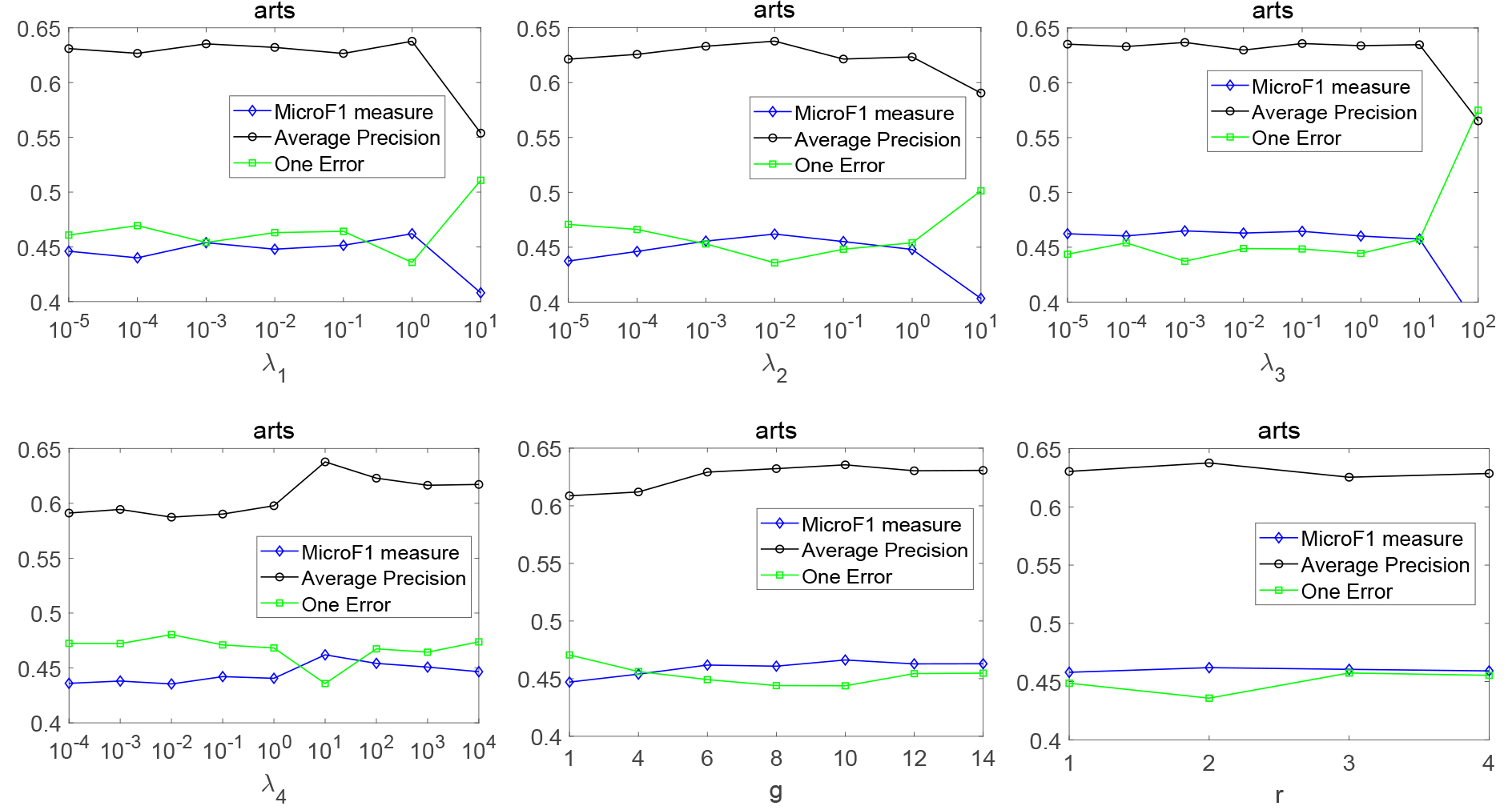
In this section, we study the sensitiveness of parameters $\lambda_{1},\lambda_{2},\lambda_{3},\lambda_{4},g$ and $r$ on LLFC, in which parameter $\lambda_{1}$ is used to control local label correlations, $\lambda_{2}$ is used to control local feature correlations, $\lambda_{3}$ is used to control the model complexity, $g$ is used to control the number of groups and $r$ is used to control the number of classifiers selected for model prediction. In this experiment, three evaluation metrics Average Precision, MicroF1 measure and One Error are selected to study parameter sensitivity on the arts data set. All parameters are analyzed according to the parameter settings in Section 4.1.2. Figure 4 shows the results of LLFC with different parameter settings.

Figure 4.

Parameter sensitivity analysis of LLFC over arts data set.

As can be seen from Fig. 4, the performance gradually increases and then decreases with the increasing of $\lambda_{1}$ and $\lambda_{2}$ . Therefore, the local label correlations and local feature correlations can improve the performance of the model. With the increasing of $\lambda_{3}$ , the performance of the model is improved to a certain extent. When $\lambda_{3}$ is too large, it may pay too much attention to the control of model complexity and ignore the training of the model, so the performance of the model is greatly reduced. The optimal performance is obtained when $\lambda_{4}$ is the intermediate value, which means that it is helpful to consider the consistency between different models for the data groups. The performance of LLFC is improved with the increasing of $g$ . When $g=$ 1, it means that there is no grouping and the global label and feature correlations are considered. However, when $g$ is too large, the number of instances and labels in the data subset may be too small to obtain reliable correlations, resulting in performance degradation. With the increase of $r$ , the performance is improved, which shows that the performance can be improved by integrating the prediction results of different models.

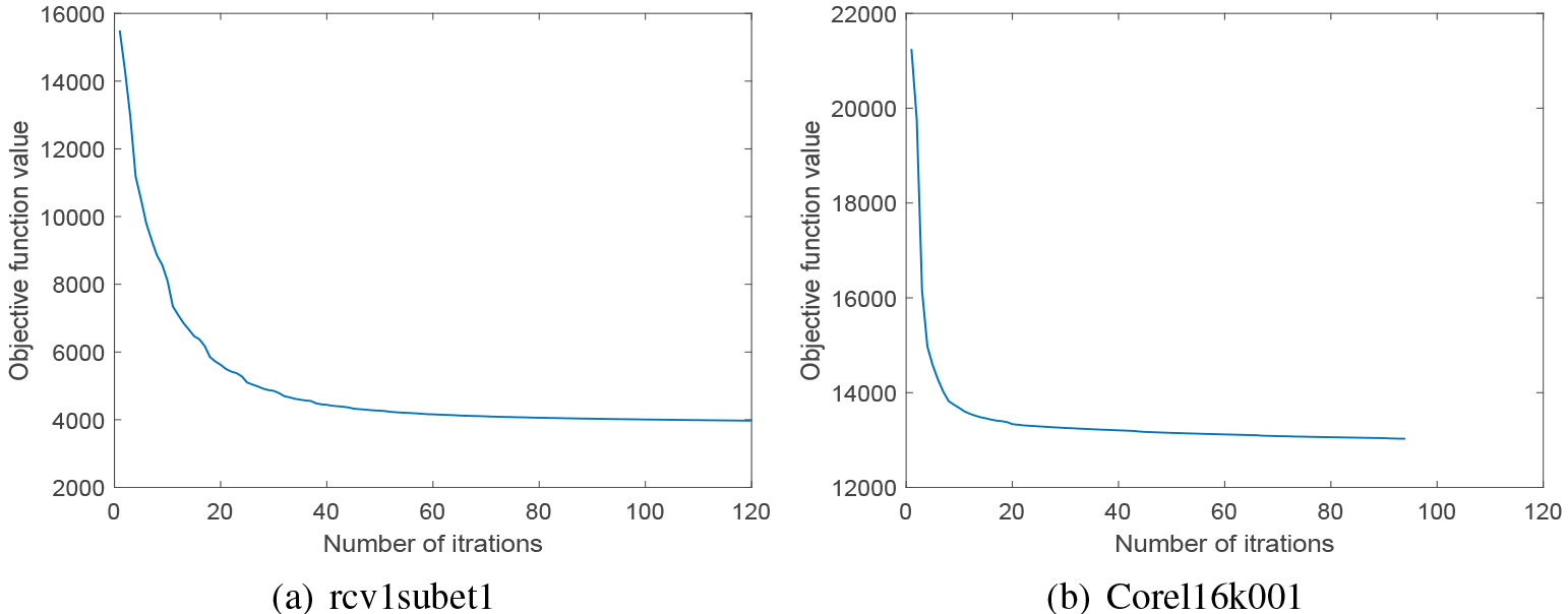
4.4 Convergence analysis

The convergence curves of our proposed method LLFC over the Corel6k001 and rcv1subset1 two data sets are shown in Fig. 5. It can be seen that the value of the objective function drops quickly and then is non-increasing.

Table 10
The running time (Sec.) costs of different algorithms,which include training and testing time

Dataset	LSF-CI	ML-LSS	GLOCAL	CLMLC	MLKNN	JFSC	LLFC
yeast	1.204	1.924	1.415	0.322	3.978	0.466	0.631
arts	11.752	21.132	9.396	0.927	18.638	20.261	11.584
corel5k	23.509	292.430	63.591	4.186	4.711	37.954	40.389
rcv1subset1	34.760	356.157	70.644	1.960	3.738	58.225	20.699
Corel16k001	93.196	713.302	70.782	7.012	14.610	155.948	64.033
Corel16k002	93.629	738.478	79.594	7.628	15.059	157.004	91.827
Stackex ${\_}$ cs	71.449	736.370	94.520	9.669	9.729	105.948	77.116
Average time(rank)	47.071(4)	408.542(7)	55.706(5)	4.529(1)	10.066(2)	76.544(6)	43.754(3)

Figure 5.

Convergence curves of the objective function value on two data sets.

4.5 Running time analysis

In this paper, the running time (including training and testing) of each algorithm on seven data sets is reported to show the efficiency of LLFC. All the algorithms are run under the same experimental environment, and the results are shown in Table 10. According to the results, LLFC ranks the third place, achieves comparable results with LSF-CI and GLOCAL, is slower than CLMLC and MLKNN, and significantly faster than ML-LSS and JFSC algorithms. That because CLMLC does not directly calculate the correlation of labels and features, and MLKNN does not consider any correlation and does not need any iterative process during the training model. ML-LSS takes a lot of time to calculate local sample correlations based on the feature of maximum label dependence. Although LLFC ranks the third place, and it achieves the best performance in multi-label classification.

5. Conclusion

In this paper, a new multi-label learning algorithm which models local label correlations and local feature correlations is proposed. The training data is divided into disjoint groups by a clustering method, and then the multi-label classifiers, the local label and feature correlations are modeled based on each data subset respectively. In addition, we model the consistency between different classifier for the data subsets. During the testing phase, prediction results of multiple classifiers are integrated together as the final prediction result. A large number of experimental results show that the proposed method is superior to many existing multi-label classification methods.

Footnotes

Acknowledgments

This work is supported by NSFC: 61806005, the University Synergy Innovation Program of Anhui Province: GXXT-2022-052, the Outstanding Young Talents Support project of Anhui Province: gxyqZD2022032, and the Natural Science Foundation of the Educational Commission of Anhui Province of China: KJ2021A0373.

References

Zhang

and Zhou

, A Review On Multi-Label Learning Algorithms, IEEE Trans. Knowl. Data Eng. 26(8) (2014), 1819–1837.

and Lv

, Multi-label text classification based on the label correlation mixture model, Intelligent Data Analysis 21(6) (2017), 1371–1392.

Almeida

A.M.G.

Cerri

Paraiso

E.C.

Mantovani

R.G.

and Junior

S.B.

, Applying multi-label techniques in emotion identification of short texts, Neurocomputing 320 (2018), 35–46. doi: 10.1016/j.neucom.2018.08.053.

Zha

and Li

, Multi-label dataless text classification with topic modeling, Knowledge and Information Systems 61(1) (2019), 137–160.

Song

and Luo

, Improving pairwise ranking for multilabel image classification, in: CVPR, 2017, pp. 1837–1845.

Tan

Shi

van den Hengel

Shen

Gao

and Zhang

, Learning Graph Structure for Multi-Label Image Classification via Clique Generation, in: CVPR, 2015, pp. 4100–4109.

Sun

Tang

G.-J.

and Huang

T.S.

, Multi-Label Image Categorization With Sparse Factor Representation, IEEE Transactions on Image Processing 23(3) (2014), 1028–1037. doi: 10.1109/TIP.2014.2298978.

Zhong

Horner

and Yang

, Music Emotion Recognition by Multi-Label Multi-Layer Multi-Instance Multi-View Learning, in: ACM, 2014, pp. 117–126.

Alzu’bi

Badarneh

Hawashin

Al-Ayyoub

Alhindawi

and Jararweh

, Multi-label emotion classification for arabic tweets, in: SNAMS, 2019, pp. 499–504. doi: 10.1109/SNAMS.2019.8931715.

10.

Zufferey

Hofer

Hennebert

Schumacher

Ingold

and Bromuri

, Performance comparison of multi-label learning algorithms on clinical data for chronic diseases, Computers in Biology and Medicine 65 (2015), 34–43.

11.

Huang

Han

Wang

Zhang

and Bhatti

U.A.

, A Clinical Decision Support Framework for Heterogeneous Data Sources, IEEE Journal of Biomedical and Health Informatics 22(6) (2018), 1824–1833. doi: 10.1109/JBHI.2018.2846626.

12.

Boutell

M.R.

Luo

Shen

and Brown

C.M.

, Learning multi-label scene classification, Pattern Recognit. 37(9) (2004), 1757–1771.

13.

Tsoumakas

Katakis

and Vlahavas

, Mining Multi-label Data, in: Data Mining and Knowledge Discovery Handbook, Springer US, 2010, pp. 667–685.

14.

Huang

and Wu

, Learning Label Specific Features for Multi-Label Classification, in: ICDM, 2015, pp. 181–190.

15.

Han

Huang

Zhang

Yang

and Feng

, Multi-Label Learning With Label Specific Features Using Correlation Information, IEEE Access 7 (2019), 11474–11484. doi: 10.1109/ACCESS.2019.2891611.

16.

Zhang

Cao

Lin

Dai

and Li

, Multi-label learning with label-specific features by resolving label correlations, Knowledge-Based Systems 159 (2018), 148–157.

17.

Tian

and Liu

, Cost-sensitive multi-label learning with positive and negative label pairwise correlations, Neural Networks 108 (2018), 411–423. doi: 10.1016/j.neunet.2018.09.003.

18.

Wang

Shen

Wang

and Chen

, Learning Low-Rank Label Correlations for Multi-label Classification with Missing Labels, in: IEEE International Conference on Data Mining (ICDM), 2014, pp. 1067–1072. doi: 10.1109/ICDM.2014.125.

19.

Huang

and Wu

, Joint Feature Selection and Classification for Multilabel Learning, IEEE Trans. Cybern. 48(3) (2018), 876–889.

20.

Zhang

Lin

Jiang

Tang

and Tan

K.C.

, Multi-label feature selection via global relevance and redundancy optimization, in: IJCAI Bessiere

, ed., 2020, pp. 2512–2518.

21.

Wang

Zheng

Cheng

and Zhao

, Joint label completion and label-specific features for multi-label learning algorithm, Soft Computing 24(9) (2020), 6553–6569.

22.

Jia

X.-Y.

Zhu

S.-S.

and Li

W.-W.

, Joint label-specific features and correlation information for multi-label learning, Computer Science and Technology 35(2) (2020), 247–258.

23.

Huang

Wang

Xue

and Huang

, Multi-label classification by exploiting local positive and negative pairwise label correlation, Neurocomputing 257 (2017), 164–174.

24.

Huang

S.-J.

and Zhou

Z.-H.

, Multi-Label Learning by Exploiting Label Correlations Locally, in: Proc. AAAI Conf. Artif. Intell, 2012, pp. 949–955.

25.

Ling

Wang

and Ling

, Exploring Common and Label-Specific Features for Multi-Label Learning With Local Label Correlations, IEEE Access 8 (2020), 50969–50982. doi: 10.1109/ACCESS.2020.2980219.

26.

Zhu

Kwok

J.T.

and Zhou

, Multi-Label Learning with Global and Local Label Correlation, IEEE Trans. Knowl. Data Eng. 30(6) (2018), 1081–1094.

27.

Weng

Lin

and Kang

, Multi-label learning based on label-specific features and local pairwise label correlation, Neurocomputing 273 (2018), 385–394. doi: 10.1016/j.neucom.2017.07.044.

28.

Zhang

Luo

Zhou

and Li

, Manifold regularized discriminative feature selection for multi-label learning, Pattern Recognition 95 (2019), 136–150. doi: 10.1016/j.patcog.2019.06.003.

29.

Gao

and Zhang

, Robust multi-label feature selection with dual-graph regularization, Knowledge-Based Systems 203 (2020), 106126. doi: 10.1016/j.knosys.2020.106126.

30.

Cai

and Zhu

, Multi-label feature selection via feature manifold learning and sparsity regularization, Int. J. Mach. Learn. Cybern. 9 (2018), 1321–1334.

31.

Jiang

Guo

and Wang

, Feature selection with missing labels based on label compression and local feature correlation, Neurocomputing 395 (2020), 95–106.

32.

Sun

Kudo

and Kimura

, A scalable clustering-based local multi-label classification method, in: Proceedings of the Twenty-Second European Conference on Artificial Intelligence(ECAI), 2016, pp. 261–268.

33.

Nasierding

Tsoumakas

and Kouzani

A.Z.

, Clustering based multi-label classification for image annotation and retrieval, in: 2009 IEEE International Conference on Systems, Man and Cybernetics, 2009, pp. 4514–4519. doi: 10.1109/ICSMC.2009.5346902.

34.

Zhou

Z.-H.

and Zhang

M.-L.

, Multi-label Learning, in: Encyclopedia of Machine Learning and Data Mining, Springer US, 2017, pp. 875–881.

35.

Zhang

M.-L.

and Wu

, Lift: Multi-Label Learning with Label-Specific Features, IEEE Transactions on Pattern Analysis and Machine Intelligence 37(1) (2015), 107–120. doi: 10.1109/TPAMI.2014.2339815.

36.

Zhang

and Zhou

, ML-kNN: A Lazy Learning Approach to Multi-Label Learning, Pattern Recognit. 40(7) (2007), 2038–2048.

37.

Elisseeff

and Jason

, A kernel method for multi-labelled classification, in: NIPS, 2001, pp. 681–687.

38.

Fürnkranz

Hüllermeier

Loza mencia

and Brinker

, Multi-label classification via calibrated label ranking, Machine Learning 73(2) (2008), 133–153.

39.

Gong

Tao

Yang

and Liu

, Teaching-to-Learn and Learning-to-Teach for Multi-label Propagation, in: AAAI, 2016, pp. 1610–1616.

40.

Huang

and Wu

, Learning Label-Specific Features and Class-Dependent Labels for Multi-Label Classification, IEEE Trans. Knowl. Data Eng. 28(12) (2016), 3309–3323.

41.

Zhang

and Zhang

, Multi-label Learning by Exploiting Label Dependency, in: KDD, 2010, pp. 999–1008.

42.

Feng

and He

, Collaboration based multi-label learning, in: AAAI, 2019, pp. 3550–3557.

43.

Tsoumakas

Katakis

and Vlahavas

, Random k-Labelsets for Multilabel Classification, IEEE Trans. Knowl. Data Eng. 23(7) (2011), 1079–1089.

44.

Read

Pfahringer

Holmes

and Frank

, Classifier Chains for Multi-label Classification, in: ECML, 2009, pp. 254–269.

45.

Cheng

and Zeng

, Joint label-specific features and label correlation for multi-label learning with missing label, Applied Intelligence 50 (2020), 4029–4049.

46.

Zhu

and Jia

, Multi-Label Learning with Local Similarity of Samples, in: 2020 International Joint Conference on Neural Networks (IJCNN), 2020, pp. 1–8. doi: 10.1109/IJCNN48605.2020.9207692.

47.

Bertsekas

D.P.

, Nonlinear Programming, Journal of the Operational Research Society 48(3) (1997), 334–334. doi: 10.1057/palgrave.jors.2600425.

48.

Demšar

, Statistical Comparisons of Classifiers over Multiple Data Sets, JMLR 7 (2006), 1–30.

Improving multi-label learning by modeling Local label and feature correlations

Abstract

Keywords

1. Introduction

3.1 Data clustering

3.2 Model construction

4. Experiment

4.1 Experimental setup

4.1.1 Data sets

1 http://mulan.sourceforge.net/datasets.html.

Table 2 Experimental results (mean ± std) of each comparison algorithm on 12 data sets in terms of Hamming Loss. ↓ indicates the smaller the value, the better the performance is. The boldface in each row indicates the best performance

Table 10 The running time (Sec.) costs of different algorithms,which include training and testing time

5. Conclusion

Footnotes

Acknowledgments

References

¹
http://mulan.sourceforge.net/datasets.html.

Table 2
Experimental results (mean $\pm$ std) of each comparison algorithm on 12 data sets in terms of Hamming Loss. $\downarrow$ indicates the smaller the value, the better the performance is. The boldface in each row indicates the best performance

Table 10
The running time (Sec.) costs of different algorithms,which include training and testing time