Machine learning techniques for received signal strength indicator prediction

Abstract

The advances made in wireless communication technology have led to efforts to improve the quality of reception, prevent poor connections and avoid disconnections between wireless and cellular devices. One of the most important steps toward preventing communication failures is to correctly estimate the received signal strength indicator (RSSI) of a wireless device. RSSI prediction is important for addressing various challenges such as localization, power control, link quality estimation, terminal connectivity estimation, and handover decisions. In this study, we compare different machine learning (ML) techniques that can be used to predict the received signal strength values of a device, given the received signal strength values of other devices in the region. We consider various ML methods, such as multi-layer ANN, K nearest neighbors, decision trees, random forest, and the K-means based method, for the prediction challenge. We checked the accuracy level of the learning process using a real dataset provided by a major national cellular operator. Our results show that the weighted K nearest neighbors algorithm, for K $=$ 3 neighbors, achieved, on average, the most accurate RSSI predictions. We conclude that in environments where the size of data is relatively small, and data of close geographical points is available, a method that predicts the coverage of a point using the coverage near geographical points can be more successful and more accurate compared with other ML methods.

Keywords

Cellular networks machine learning coverage RSSI

1. Introduction

Several decisions and planning issues in modern communication systems depend crucially on accurate coverage estimations [1]. This includes both downlink/uplink power control, handover decision algorithms, spectrum sharing, adaptive power control, distance estimation and device localization mechanism [2]. It is also useful for cellular operators to determine coverage maps of specific areas without the need for massive measurement campaigns, especially when considering multi-tier cellular networks [3].

The RSSI is an indicator of the power level received by a wireless device. RSSI decreases as the distance from the base station (BS) increases. It is complicated to estimate the RSSI value given the BS and device positions because it is affected by many other factors, including the antenna of the transmitting device, the antenna of the node itself, the number of walls, and other obstructions in the proximity of the nodes, as well as the material nature of the objects in the environment. Therefore, RSSI values exhibit high variability in space and time in real-life cellular networks in diverse environments. Moreover, one of the main reasons for the use of cellular technology is to enable devices to move freely inside the coverage area. That is, if the moving device receives low values of the RSSI, this indicates (theoretically) that the emitting device is a long distance away. Thus, it will probably exit the coverage area within a short time. Consequently, the prediction of RSSI values is very useful for predicting the disconnection of cellular devices. For this reason, it is very important to efficiently predict future RSSI values while considering the RSSI values measured nearby.

The impressive progress of ML in recent years provides a significant opportunity for the next generation of wireless networks [4, 5] to plan and build communication systems that can predict the behavior of the environment and improve network performance which finally impacts user experience. Recent studies on communication network design have suggested the use of ML methods for prediction tasks [6] and decision-making tasks [7]. Predicting RSSI using ML methods shows a great advantage over current algorithms, as these methods can be fast and adapt to changes very well, in various dynamic applications. For instance, if a new physical obstruction is located in the region, there is no need for human intervention to calibrate the algorithm since the ML method will adapt accordingly. Therefore, with proper architecture, it is possible to achieve highly accurate results. Especially in urban environments, there are many other physical effects, many of which are random in their nature. This makes the task of prediction very challenging, with many of them varying over time (that is why there is a well-known coherence time of a channel). Up to now, even the best propagation channel (that is, by the way, always adapted to a specific environment) fails to capture the real behavior of the propagation and the received signal with high accuracy. For this reason, in recent years, there have been an increasing number of studies trying to leverage the use of ML to try to predict the fundamental values for wireless networks such as RSSI with more accuracy.

However, the task of using ML methods for predicting metrics in wireless networks is challenging for several reasons. First, the required data needed for ML are not always available; data for ML should include at least thousand, and even tens and hundreds of thousands of samples, to predict the metric, while this amount of data is rarely available. Second, the considered environments change dynamically, and thus the ML method should be able to adapt to such dynamic changes. Third, the values to be predicted may depend on many factors, making the learning system more complex, which requires a complex set of input attributes for each sample data, to succeed in the learning task, while, again, such input data is not always available.

In this study, we demonstrated the efficiency of learning the RSSI values in coverage maps. For this purpose, we compared the performance of various ML methods. We consider the following ML methods: (a) a multi-layer ANN; (b) decision tree; (c) random forest, which is a combination of several binary decision trees to produce better predictive performance than utilizing a single decision tree; (d) K-means algorithm for point clustering to 100 clusters, and then calculating the expected RSSI for each cluster; (f) support vector regression (SVR); (g) K nearest neighbors (KNN) technique, which is used to predict the RSSI of points in the map using the RSSI in their neighbors. Like many recent studies [6], we propose ANNs because they are exceptionally efficient at solving nonlinear approximation problems. The KNN technique may be appropriate because the RSSI at a particular point is likely to be similar to the RSSI of its closest neighbors. However, this latter assumption should be verified, because the radio medium exhibits many stochastic phenomena that can lead to sharp fluctuations in the signal even between very close locations (e.g., the signal received before and after penetrating a concrete wall). For this reason, the KNN technique must be validated using real measurements, which we performed in this study. Comparison of different methods is important in real-time environments in which speedy learning spatial coverage maps is essential. One great advantage of our study is that we used a real dataset provided to us by a national cellular operator, whereas most existing studies rely on simulation data only.

The main contributions of this study are as follows: First, the comparison of various methods to predict RSSI, and second, the testing of the methods on real data provided by a real cellular operator. The importance of our study lies in the fact that we show how such critical challenges, namely predicting RSSI values of the type provided to us, can be performed via ML methods. In the past, this was done via a complex propagation channel, which might have limited accuracy and might not be adapted to a very dynamic environment. We provide a comparison against a relatively large number of techniques. Based on our experimental results, we conclude that given the RSSI prediction challenge in this type of coverage map, predicting the RSSI value of a point on its nearest neighbors is the most efficient prediction method and reaches the most accurate value. In particular, the method we used in the three closest neighbors, with weighting by distance, is the most accurate method for predicting RSSI values.

The remainder of this paper is organized as follows. In Section 2, we describe some background regarding the use of ML for several learning tasks in communication systems, and in Section 3, detailed information about the coverage map dataset is provided. In Section 4, we describe the ML methods used in our study and specify the training process for the networks. In particular, we provide the ANN structure used in our experiments, and we describe the preprocessing algorithm run on the provided data. In Section 5, we provide the empirical results of using ML methods to predict the RSSIs for the coverage maps dataset provided to us. Finally, in Section 7, we conclude our work and present possible directions for future work.

2. Related work

In this section, we focus on studies conducted in the area of key performance indicators in communication networks. In particular, we describe related studies for predicting the following metrics dealing with cellular network performance: signal-to-interference-plus-noise ratio (SINR) and RSSI1 Both the RSSI and SINR are sensitive to the channel response, which is the consequence of many physical effects, such as reflections and fading with distance. The main difference between SINR and RSSI is that the former considers the interference generated by other devices (transmitting at the same time in the same channel or sometimes a very close adjacent channel) and thermal noise (a non-deterministic value that depends only on the bandwidth and the temperature), whereas RSSI considers only the received signal from the desired transmitter. In the following section, we review different methods that predict both types of measurements.

Anderson and Durgin [8] characterized 3.5 GHz propagation using a series of RSS measurements that were recorded in and around St. Inigoes, Maryland, USA. Based on these data, they demonstrated that existing propagation models do not precisely and reliably describe propagation in this band. In addition, they demonstrated that even a simple geographic information system (GIS)-ased propagation model can significantly improve the propagation modeling accuracy.

Ardalani [9] used a neural network to learn the SINR in direct sequence code division multiple access systems. In his study, a neural network was trained using a series of past SINR values, which were used to predict the current SINR value for the next period. He compared single-level (Adaline) networks and multi-layer perceptron and found that both achieved tolerable estimation errors; however, by increasing the user velocity up to 120 km/h, the Adaline method achieved more accurate results. Note, however, that Ardalani’s networks learned the SINR of one period based on a series of previous SINR values, whereas, in our research, our system learns the RSSI of the coverage map given the RSSI of other points on the map. In our previous work [1, 10], we showed how to predict SIR coverage maps based on available SIR values by using several ML methods. However, the data used in [1, 10] were synthetically generated from a predefined distribution; in this study, we used RSSI coverage data provided by a major national operator.

Greenberg et al. [11] compared the accuracy of RSSI prediction using ray tracing, COST-231 HATA, and Walfisch-Ikegami models. Furthermore, they compared the accuracy of RSSI measurements provided by test drives in Ashdod and Jaffa (cities in Israel). Their results showed that deterministic ray tracing, even with site-specific digital terrain elevation data and a building layer, does not always provide more accurate predictions than empirical and physical models.

Suárez et al. [12] described the challenge of predicting future RSSI values given a past window of N-sized samples, thereby improving the decision-making process of the network entities and avoiding communication failures. For the prediction purpose, they defined a linear regression model, where the predicted value corresponded to a modified mean-reverting diffusion process. Santana et al. [2] suggest an adaptive estimation algorithm for WiFi RSSI, based on variable-size classification windows. Whenever a new measure is captured, the algorithm examines whether the new measure is consistent with the current classification window, and it generates a new window when the RSSI mean varies. They tested their estimation algorithm over time for several types of wireless equipment and concluded that their method is relevant for a wide range of devices and can also be applied to indoor localization services.

In [13], the prediction of long-range wireless signal strength was presented, where the prediction was utilized for the efficient use of resources in dynamic route selection in multihop networks. The proposed method also used past measurements of the RSSI as its input and utilized a linear regression approach, but unlike the method presented by Suárez et al. [12], it specifically addressed the problem of long-range online prediction of signal strength in wireless networks.

Chin et al. [14] revealed that typical RSSI values seem to exhibit some forms of mean-reverting behavior (converging towards a long-term mean) as well as discontinuous “jumps” (missing values for a certain period). Owing to the inherent jump properties of RSSI values, they proposed modeling this behavior using a modified Ornstein-Uhlenbeck jump diffusion process.

In the following, we survey studies utilizing ML methods for the signal prediction challenge. Sen and Gümüsay [15] integrated a multilayer feed-forward back-propagation ANN module in GIS software to interpolate the indoor electromagnetic field measurements for propagation analysis. They demonstrated that the feed-forward back-propagation ANN for spatial interpolation of electromagnetic field measurements provides adequate accuracy, but the accuracy is less than that of the predictions of Kriging interpolation [16]. However, [15] considered only one indoor coverage on the entrance floor of a building, whereas our study compared the results of outdoor coverage maps. In addition, [15] used an ANN with only one hidden layer, whereas the structure of the ANN used in our study included multiple hidden layers. However, it is worth mentioning that our conclusions are similar to that of [15], in observing that it was a challenge for the ANNs to deal with real signal predictions, probably because of the sudden discontinuities in the coverage maps.

Goudarzi et al. [17] suggested a method for RSSI prediction for ensuring seamless mobility between various network environments while minimizing the vertical handover. They use the imperialist competition algorithm to train a radial basis function (RBF) combined with the firefly algorithm (FFA) to predict the optimal solution. Similar to other previous studies, their method extrapolates RSSI values from the current time to the future, whereas in our study, we predict RSSI values in some locations based on values in other locations.

Generally, the difference between our study and most of the studies described above lies in the fact that most of the previous studies extrapolate RSSI values from the current time to the future, whereas in our study, we predict RSSI values in some locations based on values in other locations. In fact, considering the space dimension for signal predicting is more challenging, given the fact that a received signal is more prone to change in different locations at the same time than at different times in a given location.

Ozdemir et al. [18] used an ANN with two hidden layers and a feed-forward propagation algorithm called Levenberg-Marquardt to train the ANN for propagation loss prediction. The network was trained using samples with three input parameters: distance, effective antenna height, and delta-H. They found that the prediction of propagation of electromagnetic waves by the ANN was more accurate than by methods based on the Epstein-Peterson model.

Fernandes et al. [6] developed an ANN to predict the path loss of a new antenna by using information from neighboring antennas. The input data set contained, for each point, geographical information (latitude, longitude, and height), distance from that location to the BS, antenna gain at the same location, and losses that occurred between the transmission and reception. The output is the path loss value required to reach that position. They used a two-hidden-layer neural network, trained and tested on a data set from a Nordic 4G operator, where 80% of the data were used for training and 20% were used for validation. The ANN method achieved a mean absolute error of up to 6.1 dB with a standard deviation of 4 dB on the validation set, and these results show an improvement over the performance of the semi-empirical automatically calibrated standard propagation used on the same data set. The problem solved in our study is similar since we also aim to predict coverage quality of one point given the coverage quality of its surrounding neighbors. However, in our work, we compare different ML methods, to choose the best one for this particular learning challenge.

Zhang et al. [19] proposed path-loss models for an unmanned air vehicle air-to-air scenario based on ML. Ray-tracing software was employed to generate samples for multiple routes in a typical urban environment. Random forest and KNN were then used to build prediction models based on the training data. It was shown that the ML-based models can provide high prediction accuracy and acceptable computational efficiency in an air-to-air scenario. Moreover, the random forest model outperformed the other models and had the smallest prediction errors. Finally, the authors analyzed the importance of five input features for path loss in an air-to-air scenario.

In our study we demonstrate that ML methods can be successfully used for RSSI value predictions based on real data provided by a national cellular operator. In addition, in contrast with most of the aformentioned works which predict future coverage value given past values or given physical parameters, in our study we demonstrate how RSSI of a given point in the space can be predicted given its localization. We compare various ML methods, whereas existing studies use fewer methods. We note that the best way to predict the RSSI value of a point is based on the RSSI values of its neighbors. We believe that it is important to show an exhaustive comparison in order to find out what is the preferable method to deal with the stochastic behavior of wireless signals and achieve accurate predictions for efficient network management.

3. The coverage maps

Our study focuses on the opportunity to predict RSSI values using real data based on cellular technology for outdoor communication. We used a large database provided by one of the major cellular operators in Israel. For each coverage map, we were provided with the location of each base station and with the RSSI values of many points in the country. For each point, we could know with which base station it was associated, as well as to which specific sector of the BS it was associated.

In our experiments, we used 1106 coverage maps, each map represents the RSSI values for a specific BS, using cellular technology, in a particular geographical region in Israel. In particular, each coverage map was represented by an RSSI file which specifies the RSSI values of up to 1000 points in a geographical area of a specific BS. The geographical size of each coverage map was 2 km $\times$ 2 km, where each coverage map considers one base station and several sample points in the base station geographical area.

Each line in the RSSI file originally included three data fields about a specific point in the geographical coverage region of the BS, namely: the geographical point location (X, Y) according to Israel maps (considered the so-called old system of coordinates) and the RSSI value of this point. The Old Israeli grid, called also the Israeli Cassini Soldner (ICS), is the old geographic coordinate system for Israel, where (X, Y) can be translated to longitude and latitude using a linear transformation. Table 1 provides some additional information about the coverage maps used in this study, and Table 2 specifies the range of map coordinates and BS coordinates, the average RSSI values, and distance between BS and samples, calculated given the (X, Y) coordinates of the old geographic coordinate system for Israel.

Table 1
Coverage maps description

#samples	#maps	Average and (std) of RSSI value	Average coordinates range	Average BS location
1000–2499	422	$-$ 54.79 (10.01)	E:127.8, N:94.786 – E:143.682, N:111.008	E:135.077, N:102.739
2500–4999	448	$-$ 59.76 (10.8)	E:141.663, N:178.716 – E:155.538, N:192.182	E:148.023, N:184.852
5000–78000	409	$-$ 65.41 (10.55)	E:166.751, N:234.880 – E:180.643, N:249.401	E:173.226, N:241.983

Table 2

Coverage maps description – according to areas

Area	#maps	Average RSSI value	Average Euclidean distance (KM) between BS and samples
South	247	$-$ 63.48	5.125
Center	343	$-$ 58.51	4.839
North	511	$-$ 59.23	4.461

The RSSI values were measured in dBm and had typical negative values ranging between 0 dBm (excellent signal) and $-$ 110 dBm (extremely poor signal). The distance is measured in meters. A typical coverage map is depicted in Fig. 1, and a real geographical map of the area presented in Fig. 1 is presented in Fig. 2.

Figure 1.

A typical coverage map.

Figure 2.

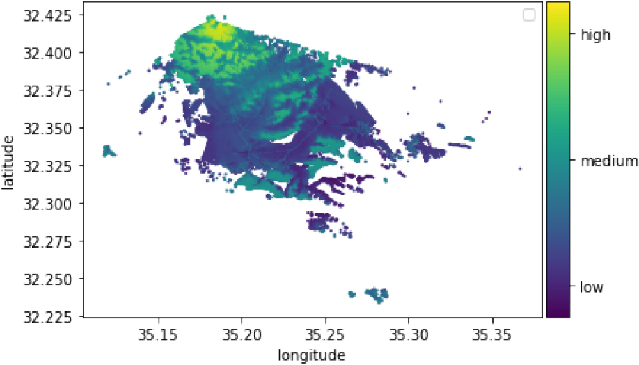
A typical coverage map with geographic background.

The coverage maps considered the RSSI values at a particular point in time. Over time, the RSSI values may change, so the sampling process and the training process should be performed periodically.

4. The RSSI prediction methods

In order to compare the accuracy of various ML methods suggested for the challenge of RSSI prediction, we divided the data for each map into a 50% training set and a 50% test set. The motivation behind the learning task discussed in this study, is to emulate a situation where some of the coverage map data is lost or damaged. Then we show how ML methods can assist us to obtain fairly accurate estimates of missing or damaged points, given the coverage information of the rest of the map. The test set points are considered as points with the damaged or lost RSSI value data, and the missing information is predicted by ML methods, using the RSSI values of the points in the training set.

For all the data items, we ran a preprocessing step, where, for each sample, we added the Euclidean distance between the sample location and the BS location, and the angle of the vertex between the sample location and the BS location, as shown in Fig. 3. These values were calculated based on the geographical location of the sample and the geographical location of the BS, which is known for each map.

Figure 3.

The angle between a sample and its base station: A demonstration.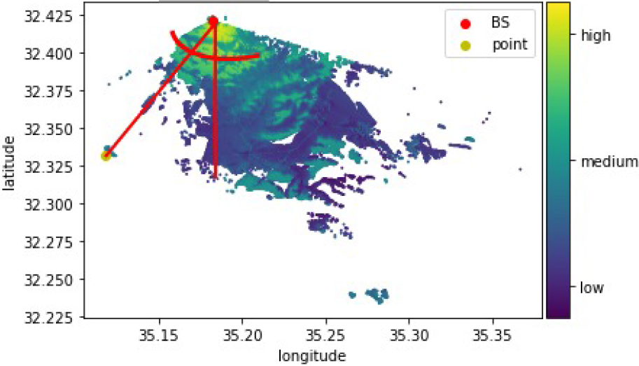

Additional data available are the locations of the BSs. Using this additional data, the distance between the point and its BS was calculated using the Euclidean distance between the point and the BS: Given $X_{BS},Y_{BS}$ which are the BS coordinates, and given $X_{p},Y_{p}$ which are the point coordinates (where we want to predict the RSSI), the Euclidean distance $\textit{distance}(BS,p)$ is calculated as

$\displaystyle\textit{distance}(BS,p)=\sqrt{(X_{BS}-X_{p})^{2}+(Y_{BS}-Y_{p})^{% 2}}$

The angle $\textit{angle}(BS,p)$ of the point w.r.t. the BS was calculated using the arctangent function of the triangle including the BS (one vertex), the sample (second vertex), and the right-angle vertex.

The angle is calculated as

$\displaystyle\textit{angle}(BS,p)=\textit{degrees}\left(\textit{arctan}\left(% \frac{X_{p}-X_{BS}}{Y_{p}-Y_{BS}}\right)\right)$

To summarize: The total features used for the RSSI prediction for each point in the coverage map are: the X-axis and the Y-axis of the point, the distance between the point and the BS, and the angle $\textit{angle}(BS,p)$ of the point w.r.t. its base station.

Then, a standard scalar transformation was performed for all the attributes and RSSI output values. The standard score of sample $x$ is calculated as follows: $z=\frac{x-u}{s}$ , where u is the mean of the training samples, and s is the standard deviation of the training samples. The details of the preprocessing step are summarized in Algorithm 3.

Row data: base station $b s$ , and samples $(x[],y[],\textit{RSSI}[])$ for the map of base station $b s$ Processed data: $\textit{scaled\_X}[],\textit{scaled\_Y}[],\textit{scaled\_distance}[],$ $\textit{scaled\_angle}[],\textit{scaled\_RSSI}[i]$ for each sample. $X_{b},Y_{b}\leftarrow$ location-of-base-station-b $\textit{sample }i\in\textit{coverage-map}$ 0.5em2em $\textit{distance}[i]\leftarrow\textit{euclidean\_distance}((x[i],y[i],bs)$ $\textit{tan}\leftarrow\textit{abs}((x[i]-bs.x)/(y[i]-bs.y))$ $\textit{angle}[i]=\textit{arctan}(\textit{tan})$ $\textit{scaled\_X}\leftarrow\textit{standard\_scale}(x)$ $\textit{scaled\_Y}\leftarrow\textit{standard\_scale}(y)$ $\textit{scaled\_distance}\leftarrow\textit{standard\_scale}(\textit{distance})$ $\textit{scaled\_angle}\leftarrow\textit{standard\_scale}(\textit{angle})$ $\textit{scaled\_RSSI}\leftarrow\textit{standard\_scale}(\textit{RSSI})$

$\textit{scaled\_X},\textit{scaled\_Y},\textit{scaled\_distance},\textit{scaled% \_angle},$ scaled_RSSI FnFunction isend standard_scale (lst: list) : list new_list $=$ [] u $=$ average (list) s $=$ stdev (list) $\textit{sample }i\in\textit{lst}$ $\textit{new\_list}[i]=(\textit{lst}[i]-u)/s$

The preprocessing algorithm

In other words, given a list, the standard scalar calculates the average and the standard deviation of the list, where each value in the list is normalized by these factors. This is performed separately for each of the attribute lists (X. Y. distances and angles), and for the RSSI values list.

After completing the preprocessing step, we ran different ML methods and compared their accuracies over the test set. We compared some classical ML methods implemented in Scikit learn [20] and ANN-based ML methods based on the Keras library [21].

In particular, we compared the results of the following ML methods:

A decision tree regressor [22]: a predictive model based on a branching series of Boolean tests that use specific facts to make more generalized conclusions. The decision tree model is efficient at handling tabular data with numerical or categorical features with fewer than hundreds of categories. Unlike linear models, decision trees can capture nonlinear interactions between the features and the target.

Random forest [23]: a collection or ensemble of simple tree predictors, each capable of producing a response when presented with a set of predictor values. In the regression problem, the responses of the decision trees were averaged to obtain an estimate of the dependent variable. Using tree ensembles can lead to significant improvements in prediction accuracy (i.e., better ability to predict new data cases).

K-nearest-neighbors regressor [24]: A “lazy learner” algorithm does not build a model using the training set until a query of the data set is performed. The value of k determines the number of neighbors to be considered in local interpolation.

Weighted K-nearest-neighbors regressor: A further refinement of the KNN method, called, the weighted KNN. According to this refinement, the neighbors’ RSSI values are weighted by the inverse of their distance from the point to predict. In this case, closer neighbors of a query point will have a greater influence than neighbors who are further away. In particular, let $\textit{NEI}_{K}(p)\subseteq\textit{POINTS}$ be the set of K nearest neighbors of point $p$ in the coverage map, the set $\textit{NEI}_{K}(p)$ of the $K$ nearest neighbors of point $p$ is calculated as follows:

$\displaystyle\textit{NEI}_{K}(p)=\textit{argmin}_{NE\subseteq\textit{POINTS},|% NE|=K}\sum_{q\in NE}{\textit{distance}(p,q)}$

The weight of each point is calculated as

$\displaystyle\textit{weight}(\textit{neighbor},p)=1/\textit{distance}(p,% \textit{neighbor})$

and the predicted RSSI value of $p$ is calculated as follows:

$\displaystyle\textit{predicted\_RSSI}(p)=\frac{\sum_{\textit{q in NEI}_{K}(p)}% \textit{weight}(q,p)\times\textit{RSSI}(q)}{\sum_{\textit{q in NEI}_{K}(p)}% \textit{weight}(q,p)}$

In fact, the weighted KNN method, using three nearest neighbors, reached the most accurate prediction for RSSI values in our study, as described in Table 5, Section 5.

K-means clustering-based regressor [25]: an unsupervised clustering method, which we used as follows. The training set was divided into 100 clusters, and each point in the test set was associated with the nearest cluster. Finally, the predicted RSSI value was evaluated as the average RSSI value of the training set points that were associated with the same cluster.

Figure 4.

Proposed neural network structure – graphical view.

Support vector machine (SVM) – based method [26]: tries to fit the best line within a predefined or threshold error value. In our study, we used the radial basis function (RBF) kernel with $\textit{gamma}=\textit{scale}$ , and the default values of the other parameters. This means that the kernel function is defined as $\exp(-\textit{gamma}\times||x-x^{\prime}||^{2})$ , and the value of gamma is defined as $1/(n_{f}\textit{eatures}*\textit{var}(x))$ .

Multi-layer ANN: An ANN consists of a collection of simulated neurons that are connected in a way inspired by biological neural networks. The operations performed in the neural network are usually defined by a weighted combination of a specific group of units with a nonlinear activation function, depending on the structure of the model [4]. In the current study, we tried different structures of ANN, and finally, we used and tested the following ANN structure, which achieved the most promising accuracy. The best network we used had three hidden layers: 256 ReLu neurons in the input layer, 128 ReLu neurons in the first and second hidden layers, and 32 ReLu neurons in the third layer, with one identity output neuron. The Adam optimizer was used, and the mean squared error served as the loss function. The neural network structure is shown in Figs 4 and 5. Unless otherwise specified, the ANN was trained using 100 epochs, relative batch size (0.5% of the number of samples for coverage maps with less than 10K samples, and 0.2% for larger maps), and learning rate $=$ 0.001.

5. Experimental results

As explained above, we obtained access to a big database provided by a major national cellular operator (access to part of this database can be provided upon request). In this section, we present the accuracy of the various ML methods, described in Section 4, on the coverage maps database. For each coverage map, 50% of the sampled users’ locations were used for the training set, and the other 50% used as the test set, to check the accuracy of the trained ML method on new unseen users’ locations. In particular, to check the accuracy of the results, we used the following error metrics: (a) Average and standard deviation of the absolute error: For each sample, we computed the absolute error of the learned RSS with respect to the real RSS. (b) Average and standard deviation of the square root of the mean squared error (RMSE) for each prediction, and we show the average and standard deviation of the RMSE values. The RMSE value was calculated as follows:

$\displaystyle\textit{RMSE}=\sqrt{\frac{\Sigma_{i=1}^{n}(y_{\textit{real}}-y_{% \textit{predicted}})^{2}}{n}}$

We used the above metrics, which are the classical quality measurements for the solution quality of regression problems, where RMSE is more affected by extreme values. We proceed by comparing the metrics results of classical ML methods on the RSSI prediction challenge.

Table 3
Comparison of the different classical ML methods

Method	RMSE: mean (std)	Absolute error: mean (std)
KNN	3.92 (1.73)	2.05 (1.27)
Decision tree	4.66 (2.1)	2.32 (1.47)
Random forest	4.75 (2.35)	3.23 (2.02)
SVM	5.55 (2.91)	3.63 (2.41)
ANN	4.1 (1.85)	2.56 (1.52)
K-means	4.97 (2.35)	3.2 (1.96)

Figure 5.

Proposed neural network structure – another description.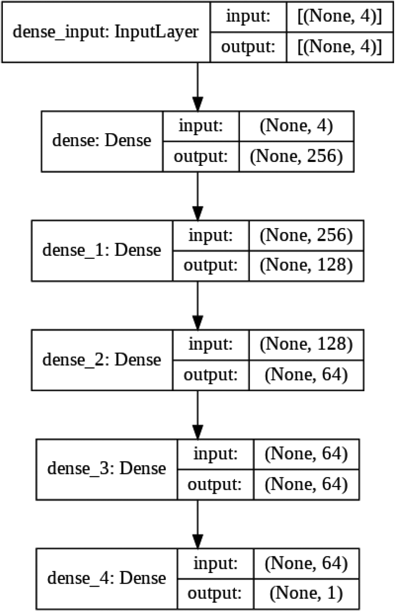

As shown in Table 3, the best method was the KNN, while the other learning methods yielded far less accurate results, according to both types of metrics: namely average error, and mean squared error, the results were lower when using KNN w.r.t. the other methods. Note that the KNN method uses the data of the k-nearest points to predict the value of the predicted point. This method achieved the best results for most of the maps. While other methods use generalization and fail to predict sudden changes in the map, the KNN, which looks at the nearest neighbors of each point, can easily predict values more accurately by recognizing such sudden changes given the KNN of each point.

Subsequently, we checked whether the comparison of these three methods changed for different map sizes. Figs 6 and 7 present the results of the KNN and ANN methods over the various coverage maps, that were divided into three groups, according to their sizes.

Figure 6.

Absolute error for the RSSI prediction of KNN and ANN, with the maps categorized by their size (number of points).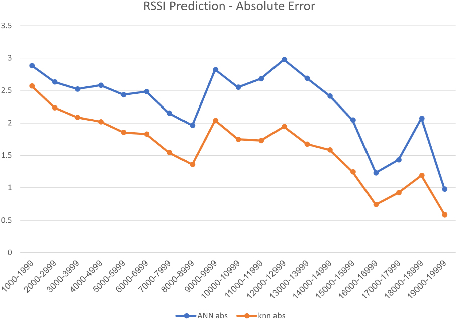

As can be seen, for all coverage maps that include up to 3000 points, KNN is the most accurate method. This can be explained by the fact that in all coverage maps, the higher the number of points on the map, the higher the map density; thus, the KNN could better predict the RSSI value of a point given the neighbors’ point.

5.1 Comparing the accuracy of the various ML methods

We proceed by training the learning methods without using additional attributes (distance from the BS and angle of the vertex between the sample point and the BS). We compared the performance of the following ML methods: (a) an ANN trained by all four attributes (X, Y, distance from base station, and angle), different types of activation functions: three hidden layers: 256 neurons in the first layer, 128 neurons in the second layer, 128 neurons in the third layer, and 32 neurons in the fourth layer. The activation function was tanh, and the Adam optimizer was used for 500 epochs with a batch size of 64. (b) ANN with the same structure and optimization method, trained only by the original attributes (X, Y), (c) KNN method, using four nearest neighbors, where the neighborhood was calculated using the four attributes, X, Y, distance, and angle with respect to the base station. (c) KNN method, using four nearest neighbors, where the neighborhood was calculated using only the X and Y values and tanh activation function used in all neural network layers. Table 4 provides our results.

Table 4
Comparison of the ANN and the KNN methods

	ANN	ANN, with distance & angle	KNN	KNN, with distance & angle
Average absolute error std	2.27 (1.29)	2.25 (1.29)	2.04 (1.25)	2.10 (1.29)
Average squared error std	3.85 (1.67)	3.87 (1.69)	3.72 (1.64)	3.81 (1.68)

Figure 7.

RSME for the RSSI prediction of KNN and ANN, with the maps categorized by their size (number of points).

We can see that when using KNN, the results using only the X and Y values were more accurate for the KNN results than when using the four attributes, whereas in the ANN, adding the distance from the base station and the angle did not change the quality of the results. In another experiment, we attempted to use the sigmoid activation function instead of tanh activation methods, resulting in an increase in the ANN error, with an average absolute error of 2.88 instead of 2.25, (stdev 1.788), and an average squared error of 4.413 instead of 3.87 (stdev 2.11). In any case, the KNN (using two nearest neighbors with uniform weights) achieved more accurate results with respect to the ANN method.

Given the superiority of using only (X, Y) attributes for the KNN, we checked again the KNN performance for different numbers of neighbors and compared the results of using the weighted average of the nearest neighbors with the results of using the uniform (unweighted) average of the nearest neighbors. The performance results are listed in Table 5.

Table 5

Comparison of different variations of the KNN method

K	Uniform neighbours		Weighted neighbours
	abs. error	sq. error	abs. error	sq. error
2	2.00 (1.24)	3.84 (1.70)	1.95 (1.21)	3.80 (1.68)
3	2.00 (1.24)	3.73 (1.65)	1.92 (1.19)	3.65 (1.62)
4	2.04 (1.25)	3.72 (1.64)	1.93 (1.19)	3.6 (1.59)
5	2.09 (1.28)	3.73 (1.65)	1.95 (1.20)	3.59 (1.58)
6	2.13 (1.31)	3.77 (1.67)	1.98 (1.21)	3.59 (1.59)
7	2.18 (1.34)	3.81 (1.69)	2.00 (1.23)	3.60 (1.59)
8	2.22 (1.36)	3.85 (1.71)	2.03 (1.24)	3.62 (1.60)
9	2.27 (1.39)	3.89 (1.73)	2.06 (1.26)	3.64 (1.61)
10	2.31 (1.42)	3.93 (1.75)	2.08 (1.28)	3.66 (1.62)

We can observe that the weighted variation, where a weighted average is used for the RSSI evaluation, yields slightly better results than the uniform variation, and that the model with three neighbors reached, in general, the most accurate results. The average absolute error of the KNN regressor, for different numbers of neighbors and both average variations (weighted or uniform), is presented in Fig. 8. It can be observed that the most accurate RSSI prediction is reached for the weighted average calculation of the three nearest neighbors, and this result outperforms the results of any other method we tested in this work. In fact, the superiority of a relatively small number of neighbors lies in the fact that when using more neighbors, points that are farther from the point being studied are taken into account. This reduces the accuracy of the results. No other method, including different ANN variations we tried, could outperform the above performance of the KNN method.

Figure 8.

The performance of the KNN regressor.

In some of the coverage maps, early stopping can be efficient, but we did not observe overfitting behavior during the training process. A typical convergence process is presented in Fig. 9. It can be observed that, after the first 100 epochs, the rest of the training is redundant. By observing the training process in other coverage maps, we found some maps where the accuracy was improved also after the first 100 epochs, but, in fact, the effectiveness of the training steps after it was relatively negligible.

Figure 9.

A typical convergence of the training set loss and the validation set loss over epochs.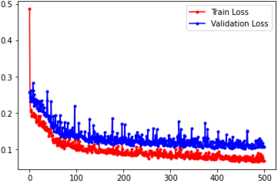

We tried also several variations of ANNs trained by the K nearest neighbors of the users’ locations, but in general, we found in all our experiments that the simple KNN outperformed all other methods. To summarize, our experiments demonstrate that the KNN method outperformed all ANN variations we checked. Given the above results, we can conclude that the task of predicting RSSI values in cellular coverage maps can be performed successfully and that the most accurate results are achieved when using KNN or ANN-based methods, with a clear superiority of the weighted KNN method, with three nearest neighbors taken for RSSI prediction. This method outperformed all other methods that we have tried.

6. Discussion of our results

In this study, we used RSSI coverage maps, provided by a major national cellular operator, and we examined the efficiency of various ML methods on learning the RSSI values at some points in the space given a partial map of the coverage. The methods we applied were: an ANN, a decision tree, random forest, and K-means based algorithm with dividing the data into 100 clusters, where the average RSSI value of each cluster was used for RSSI prediction, SVR with RBN kernel, KNN method, and weighted KNN methods. Our results from various experiments demonstrated that the most effective method is the weighted K nearest neighbors method, when considering the three closest neighbors, and calculating the RSSI as a weighted average of the neighbors RSSI’s, weighted by a function of their distance from the predicted point. This method achieved, by average, the most accurate RSSI predictions.

It should be noted that the KNN method is called a lazy method, and its disadvantages lie in the fact that when it is applied over a given set of samples, the process of finding the K nearest samples may be expensive. However, in the wireless domain, online finding the nearest neighbors of a user may be performed efficiently. Therefore, even when looking at the time and place complexity required for online RSSI prediction, the KNN method still outperforms the neural network method in the environments we are talking about.

It should be emphasized that the experiments we ran were on data from relatively small coverage maps, and our conclusion is that the best learning was the one that drew conclusions about the RSSI values of a point based on the RSSI values of its nearest neighbors. If we consider additional data about the users’ locations, such as the topographical attributes and the building in their area, then, of course, it will improve the ANN accuracy. But assuming that this additional information is not available, it turns out that the KNN method provides a superior solution in terms of both efficiency and quality.

Our conclusion from the results of our experiments is that in environments where the size of data is relatively small, and where points that are close are relatively similar, a method that predicts the coverage of a point using only coverage in close geographical points can be more successful and accurate than more advanced methods.

In addition, in terms of efficiency, this method does not require time of training, compared to the training of a neural network. Moreover, the time required to reach some conclusion is relatively reasonable and not so different than the time required if using a deep network. Therefore, the nearest neighbors method can be the preferred method for learning unknown points for maps on the order of thousands or tens of thousands of data, where except for individual discontinuous areas, the coverage of a point can be deduced based on coverage in nearby areas.

7. Conclusion

In this study, we show how critical challenges, namely, predicting RSSI values can be performed via ML methods. This has been done in the past via a complex propagation channel, which might have limited accuracy and might not be adapted to a very dynamic environment. We used RSSI coverage files provided by a major national cellular operator and tested the ability of ML to predict RSSI values on a coverage map based on data about other RSSI values. We divided each coverage file into two sets, 50% as the training set and 50% as the test set. We fed different ML methods with training set samples, and then checked the accuracy of the ML predictions on the test set. We compared the following methods: a multilayer ANN model, KNN, decision tree, random forest, SVM, and the K-means-based method. We found that, on average, the two best methods were the KNN and the ANN. In addition, our results from various experiments demonstrate that KNN is the most accurate prediction method.

The main reason for the advantage of the KNN over the ANN relies on the fact that the only information we were provided was the coordinates (X, Y) of each point, from which we deduced the distance values from the BS and the angle. We did not have access to additional information for each point such as its height, surrounding building in its area, and the transmission power of the BS. Thus, it turns out to be quite natural that according to this limited information, the best means of predicting RSSI at a given point is indeed its neighbors.

To the best of our knowledge, there are few studies that validate their results against real data provided by real cellular operators. Most existing works rely on the results generated by simulators and/or experimental labs. Furthermore, we provide a comparison of ML methods against a relatively large number of techniques, whereas many other studies use only one or two techniques.

In future work, we would like to consider learning methods to predict signal strength given data based on real “trips” of people measuring their signal strength. In addition, we would like to consider the time dimension, that is, the signal strength prediction over time.

Footnotes

RSSI and RSS are equivalent. RSSI is the RSS with the word indicator at the end.

References

Rozenblit

Y.M.O.

Haddad

and Azoulay

, Machine learning methods for SIR prediction in cellular networks, Physical Communciation 31 (2018), 239–253.

Santana

J.A.

Macías

Suarez

Á.

Marrero

and Mena

, Adaptive estimation of WiFi RSSI and its impact over advanced wireless services, Mobile Networks and Applications 22 (2017), 1100–1112.

Haddad

and Porrat

, A two-tier frequency reuse scheme, in: 2010 IEEE 21st International Symposium on Personal, Indoor and Mobile Radio Communications Workshops, 2010, pp. 203–207.

Zhang

Patras

and Haddadi

, Deep learning in mobile and wireless networking: A survey, IEEE Communications Surveys Tutorials 21(3) (2019), 2224–2287.

Sun

Peng

Zhou

Huang

and Mao

, Application of machine learning in wireless networks: Key techniques and open issues, IEEE Communications Surveys Tutorials 21(4) (2019), 3072–3108.

Fernandes

D.F.S.

Raimundo

Cercas

SebastiÃ£o

P.J.A.

Dinis

and Ferreira

L.S.

, Comparison of artificial intelligence and semi-empirical methodologies for estimation of coverage in mobile networks, IEEE Access 8 (2020), 139803–139812.

Liang

and Li

G.Y.

, Deep-learning-based wireless resource allocation with application to vehicular networks, Proceedings of the IEEE 108(2) (2020), 341–356.

Anderson

C.R.

and Durgin

G.D.

, Propagation measurements and modeling techniques for 3.5 GHz radar-LTE spectrum sharing, in: 2017 XXXIInd General Assembly and Scientific Symposium of the International Union of Radio Science (URSI GASS), 2017, pp. 1–4.

Ardalani

, SINR prediction in mobile CDMA systems by linear and nonlinear artificial neural-network-based predictors, IJCSI International Journal of Computer Science Issues 8(4) (2011), 220–228.

10.

Mirsky

O.R.Y.

Haddad

and Azoulay

, Predicting wireless coverage maps using Radial Basis Network, in: CCNC, 2018, pp. 1–4.

11.

Greenberg

and Klodzh

, Comparison of Deterministic, Empirical and Physical Propagation Models in Urban Environments, in: COMCAS, 2015, pp. 1–5.

12.

Suárez

Santana

J.A.

Macias-Lopez

E.M.

Mena

V.E.

Canino

J.M.

and Marrero

, RSSI prediction in WiFi considering realistic heterogeneous restrictions, Network Protocols and Algorithms 6(4) (2014), 220–228.

13.

S.X. Long B, A Real-Time Algorithm for Long Range Signal Strength Prediction in Wireless Networks, IEEE Wireless Communications and Networking, 2008, 1120–1125.

14.

Chin

Chieng

Teh

Natkaniec

Loziak

and Gozdecki

, Wireless link prediction and triggering using modified Ornstein-Uhlenbeck jump diffusion process, Wireless Networks 20(3) (2014), 379–396.

15.

Sen

A.K.A.

Gümüsay

M.U.

and Bulucu

, Programming an Artificial Neural Network Tool for Spatial Interpolation in GIS – A Case Study for Indoor Radio Wave Propagation of WLAN, Sensors 8(9) (2008).

16.

Tatalovich

Wilson

J.P.

and Cockburn

, A comparison of thiessen polygon, kriging, and spline models of potential UV exposure, Cartography and Geographic Information Science 33(3) (2006), 217–231.

17.

Goudarzi

Hassan

W.H.

Hashim

A.-H.A.

Soleymani

S.A.

Anisi

M.H.

and Zakaria

O.M.

, A novel RSSI prediction using imperialist competition algorithm (ICA), radial basis function (RBF) and firefly algorithm (FFA) in wireless networks, PLoS ONE 11(7) (2016), 379–396.

18.

Ozdemir

A.R.

Alkan

Kabak

Gulsen

and Sazli

M.H.

, The prediction of propagation loss of FM radio station using artificial neural network, Journal of Electromagnetic Analysis and Applications 6 (2014), 358–365.

19.

Zhang

Wen

Yang

and Luo

, Air-to-air path loss prediction based on machine learning methods in urban environments, Wireless Communications and Mobile Computing 2018 (2018), 1–9.

20.

Scikit Learn, [Online], 2020 (accessed June 21, 2020). https://scikit-learn.org.

21.

Keras, [Online], 2020 (accessed June 21, 2020). https://keras.io/.

22.

Russel

and Norvig

, Learning Decision Trees, in: Artificial Intelligence, a Modern Approach, 3rd edition, John Wiley and Sons, 2010, pp. 697–707, Chapter 18.3.

23.

Breiman

, Random forests, Machine Learning 45(1) (2001), 5–32.

24.

Chen

G.H.

and Shah

, Explaining the success of nearest neighbor methods in prediction, Foundations and Trends in Machine Learning 10(5–6) (2018), 337–588.

25.

Macqueen

, Some methods for classification and analysis of multivariate observations, in: In 5-th Berkeley Symposium on Mathematical Statistics and Probability, 1967, pp. 281–297.

26.

Cortes

and Vapnik

V.N.

, Support-vector networks, Machine Learning 20(3) (1995), 273–297.

27.

Zaidi

S.A.R.

, Nearest neighbour methods and their applications in design of 5G & beyond wireless networks, ICT Express 7(4) (2021), 414–420.

28.

Farjow

Chehri

Hussein

and Fernando

, Support Vector Machines for indoor sensor localization, in: 2011 IEEE Wireless Communications and Networking Conference, 2011, pp. 779–783. doi: 10.1109/WCNC.2011.5779231.

29.

Nguyen

C.L.

Georgiou

and Suppakitpaisarn

, Improved Localization Accuracy Using Machine Learning: Predicting and Refining RSS Measurements, in: 2018 IEEE Globecom Workshops (GC Wkshps), 2018, pp. 1–7.

30.

Feng

Minghua

Jing

Xiao

Ming

Tao

and Xinrong

, An Improved Indoor Localization of WiFi based on support vector machines, International Journal of Future Generation Communication and Networking 7(5) (2014), 191–2016.

31.

Bhatti

, Machine learning based localization in large-scale wireless sensor networks, Sensors 18(12) (2018). https://www-mdpi-com-s.web.bisu.edu.cn/1424-8220/18/12/4179.

32.

Chriki

Touati

and Snoussi

, SVM-based indoor localization in Wireless Sensor Networks, in: 2017 13th International Wireless Communications and Mobile Computing Conference (IWCMC), 2017, pp. 1144–1149.

33.

Seyed Saber Banihashemian

F.A.

and Sarram

M.A.

, A new range-free and storage-efficient localization algorithm using neural networks in wireless sensor networks, Wireless Personal Communications 98 (2018), 1547–1568.

34.

Zhu

and Wei

, Localization algorithm for large-scale wireless sensor networks based on FCMTSR-support vector machine, International Journal of Distributed Sensor Networks 12(10) (2016).

35.

Khatab

Z.E.

Hajihoseini

and Ghorashi

S.A.

, A fingerprint method for indoor localization using autoencoder based deep extreme learning machine, IEEE Sensors Letters 2(1) (2018), 1–4.

36.

Nguyen

C.L.

Georgiou

and Suppakitpaisarn

, Improved Localization Accuracy Using Machine Learning: Predicting and Refining RSS Measurements, in: 2018 IEEE Globecom Workshops (GC Wkshps), 2018, pp. 1–7.

37.

Ahmadi

and Bouallegue

, Exploiting machine learning strategies and RSSI for localization in wireless sensor networks: A survey, in: 2017 13th International Wireless Communications and Mobile Computing Conference (IWCMC), 2017, pp. 1150–1154.

38.

Samadian

and Noorhosseini

S.M.

, Probabilistic support vector machine localization in wireless sensor networks, ETRI Journal 33(6) (2011), 924–934.

39.

X.L. Rauchenstein Lynn T. and Abhinav Vishnu and Deng

Z.D.

, Improving underwater localization accuracy with machine learning, Review of Scientific Instruments 89(7) (2018).

40.

Phillips

Sicker

and Grunwald

, A survey of wireless path loss prediction and coverage mapping methods, IEEE Communications Surveys Tutorials 15(1) (2013), 255–270.

41.

Cheng

and Shen

, An Improved Recurrent Neural Network for Radio Propagation Loss Prediction, in: 2010 International Conference on Intelligent Computation Technology and Automation, Vol. 1, 2010, pp. 579–582.

42.

Popescu

Nikitopoulos

Constantinou

and Nafornita

, Comparison of ANN Based Models for Path Loss Prediction in Indoor Environment, in: IEEE Vehicular Technology Conference, 2006, pp. 1–5.

43.

Mom

C.O.M.J.M.

and Igwue

G.A.

, Application of artificial neural network for path loss prediction, Urban Macrocellular Environment, American Journal of Engineering Research (AJER) 3(2) (2014), 270–275.

44.

Isabona

and Srivastava

V.M.

, A neural network based model for signal coverage propagation loss prediction in urban radio communication environment, International Journal of Applied Engineering Research 11(22) (2016), 11002–11008.

45.

Alqudah

Y.A.

Sababha

Elnashar

and Sababha

S.H.

, On the validation of path loss models based on field measurements using 800 MHz LTE network, in: 2016 Annual IEEE Systems Conference (SysCon), 2016, pp. 1–5.

46.

Imoize

P.O.N.A.L.

Ibhaze

A.E.

and Ajose

S.O.

, Determination of Best-fit Propagation Models for Pathloss Prediction of a 4G LTE Network in Suburban and Urban Areas of Lagos, Nigeria, The West Indian Journal of Engineering 41(2) (2019), 13–21.

47.

Imoize

A.L.

and Ogunfuwa

T.E.

, Propagation Measurements of a 4G LTE Network in Lagoon Environmenta, Nigerian Journal of Technological Development 16(1) (2019).

48.

Egi

and Otero

C.E.

, Machine-Learning and 3D Point-Cloud Based Signal Power Path Loss Model for the Deployment of Wireless Communication Systems, IEEE Access 7 (2019), 42507–42517.

49.

Bkassiny

and Jayaweera

S.K.

, A survey on machine-learning techniques in Cognitive Radios, IEEE Communication Surveys and Tutorials 15(3) (2013), 1136–1159.

50.

O’Shea

and Hoydis

, An introduction to deep learning for the physical layer, IEEE Transactions on Cognitive Communications and Networking 3(4) (2017), 563–575.

51.

Tumuluru

V.K.

Wang

and Niyato

, A Neural Network Based Spectrum Prediction Scheme for Cognitive Radio, in: 2010 IEEE International Conference on Communications, 2010, pp. 1–5.

52.

Wang

L.M.Y.

Zhang

and Chen

, SVM-based spectrum mobility prediction scheme in mobile cognitive radio networks, The Scientific World Journal 2014 (2014).

53.

Chang

P.-R.

and Yang

W.-H.

, Environment-adaptation mobile radio propagation prediction using radial basis function neural networks, IEEE Transactions on Vehicular Technology 46(1) (1997), 155–160.

54.

Iliya

Goodyer

Gow

Shell

and Gongora

, Application of Artificial Neural Network and Support Vector Regression in cognitive radio networks for RF power prediction using compact differential evolution algorithm, in: 2015 Federated Conference on Computer Science and Information Systems (FedCSIS), 2015, pp. 55–66.

55.

Guerriero

P.P.F.

Loscrí

and Surace

, Neural Networks and SDR Modulation schemes for wireless mobile nodes: A synergic approach, Ad Hoc Networks 54 (2017), 17–29.

56.

Dong

and Cai

, A learner based on neural network for cognitive radio, in: 2010 IEEE 12th International Conference on Communication Technology, 2010, pp. 893–896.

57.

Schmidhuber

, Deep learning in neural networks: An overview, Neural Networks 61 (2015), 85–117.

Machine learning techniques for received signal strength indicator prediction

Abstract

Keywords

1. Introduction

2. Related work

3. The coverage maps

Table 1 Coverage maps description

Table 3 Comparison of the different classical ML methods

Table 4 Comparison of the ANN and the KNN methods

7. Conclusion

Footnotes

References

Table 1
Coverage maps description

Table 3
Comparison of the different classical ML methods

Table 4
Comparison of the ANN and the KNN methods