Learning bayesian multinets from labeled and unlabeled data for knowledge representation

Abstract

The Bayesian network classifiers (BNCs) learned from labeled training data are expected to generalize to fit unlabeled testing data based on the independent and identically distributed (i.i.d.) assumption, whereas the asymmetric independence assertion demonstrates the uncertainty of significance of dependency or independency relationships mined from data. A highly scalable BNC should form a distinct decision boundary that can be especially tailored to specific testing instance for knowledge representation. To address the issue of asymmetric independence assertion, in this paper we propose to learn k-dependence Bayesian multinet classifiers in the framework of multistage classification. By partitioning training set and pseudo training set according to high-confidence class labels, the dependency or independency relationships can be fully mined and represented in the topologies of the committee members. Extensive experimental results indicate that the proposed algorithm achieves competitive classification performance compared to single-topology BNCs (e.g., CFWNB, AIWNB and SKDB) and ensemble BNCs (e.g., WATAN, SA2DE, ATODE and SLB) in terms of zero-one loss, root mean square error (RMSE), Friedman test and Nemenyi test.

Keywords

Bayesian network classifier Asymmetric independence assertion k-dependence Bayesian multinet classifier Multistage classification

1. Introduction

Classification is one of the key issues in machine learning and data mining [1, 2, 3]. Researchers propose to learn Bayesian network classifiers (BNCs) [4, 5] for classification and knowledge representation under condition of uncertainty. According to multivariate data analysis across disciplines, the learning procedure of BNCs can be divided into two parts: structure learning that models data in the form of directed acyclic graph (DAG), and parameter learning that estimates the joint probability based on the learned DAG. However, learning an optimal DAG from existent data is NP-hard [6].

Most learning algorithms assume that the instances for training are independently and identically distributed (i.i.d.) [7, 8]. That is, if the statistical model learned from training data can achieve the right estimate of probability distributions, then it can also fit each unseen instance from the testing data. Obviously this assumption is too tight for many applications[9, 10], and that may result in negative influence on the generalization performance [11]. By combining multiple models, an ensemble learner (e.g., Random Forest [12], AODE [13, 14] and AdaBoost [15]) can compensate the errors produced by any one of its members [16], and it works especially when the probability distributions learned from labeled training set as input can generalize to the testing data. In contrast, instance learning mines significant dependency relationships among random variables implicated in each instance, and the learned probability distributions can hopefully fit each instance if the wrong class labels are not introduced into the learning procedure.

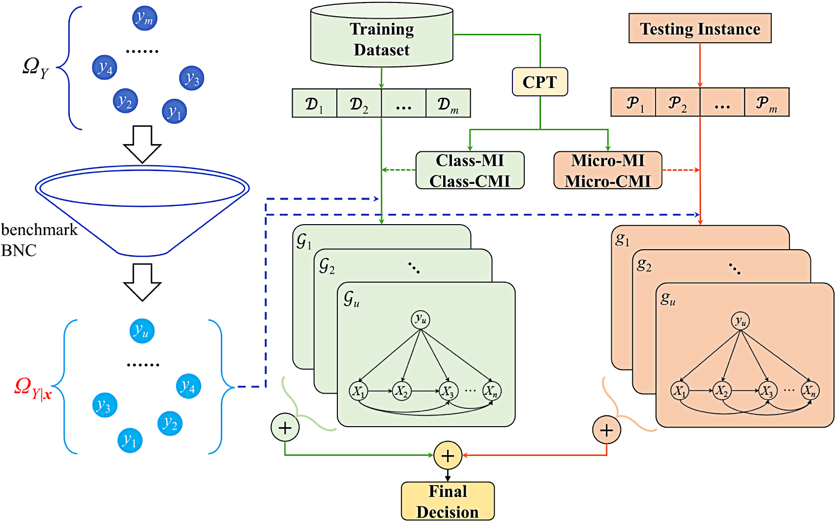
For specific unlabeled instance, sometimes it is hard to differentiate one class label from the others among the most possible high-confidence ones. By removing the class labels with low-confidence information to alleviate the conditional independence assumption, the estimates of information-theoretic metrics will be calibrated and that may help enhance the robustness of the learned network topology [17]. Furthermore, labeled training data and unlabeled testing data both contribute to the completeness of knowledge, and when they work jointly to learn the right probability distribution, the final BNC will achieve the bias/variance trade-off. In this paper we propose to filter out low-confidence class labels and then build a Bayesian multinet classifier (BMC), called class-specific Bayesian classifier (CSB), which consists of two sets of class-specific BNCs in the framework of multistage learning [18]. The main contributions are as follows:

•
Class-specific information-theoretic metrics, e.g., Class-CMI or Micro-CMI, are introduced to identify asymmetric (conditional) dependence between attributes or attribute values. To improve the generalization performance, the training set and pseudo training set are partitioned according to high-confidence class labels, then local BNCs can be learned from each subset and fully represent the dependency or independency relationships implicated. The resulting highly scalable BMC learns an ensemble of class-specific k-dependence Bayesian classifiers in the framework of multistage classification.
•
We compare the performance of our BMC with single-topology BNCs (e.g., CFWNB, AIWNB and SKDB) and ensemble BNCs (e.g., WATAN, SA2DE, ATODE and SLB). The local BNCs learned from training subsets or pseudo training subsets demonstrate significant advantage over KDB when they work independently or jointly. The experimental results of Friedman test [49] and Nemenyi statistics [50] show that our algorithm achieves competitive generalization performance while dealing with 28 datasets from different research domains, ranging in size from 32 to 1,025,010 instances and 4 to 64 attributes.

The rest of this paper is organized as follows: Section 2 briefly introduces the i.i.d. assumption for learning BNC and the framework of multistage classification. The basic idea and detailed learning procedure of CSB are described in Section 3. The experimental results of CSB and the comparisons with a set of state-of-the-art BNCs are presented in Section 4. To finalize, Section 5 shows the main conclusions and outlines future work.
2. Background knowledge

Table 1 lists all the symbols which are used in this paper.

Table 1
List of symbols used in this paper

Notation	Description
$P(\cdot)$	Estimate of probability distribution
$X_{i}$	Predictive attribute (or random variable)
$x_{i}$	Discrete values for attribute $X_{i}$
${\bm{x}}=\{x_{1},\ldots,x_{n}\}$	An instance of $n$ -dimensional vector
$Y$	Class variable
$y$	Discrete values for $Y$
$\Omega_{Y}$	Set of labels of the class variable $Y$
$N$	Number of training instances
$M$	Number of testing instances
$n$	Number of predictive attributes
$m$	Number of classes

2.1 Bayesian network classifiers

In the DAG of BNC over predictive attributes $\{X_{1},\ldots,X_{n}\}$ and class variable $Y$ , each node denotes an attribute or the class variable, and arcs connecting the attribute nodes represent (conditional) dependencies between them. Thus the (conditional) independence is denoted by the lack of arc connecting specific nodes. The conditional probability for attribute $X_{i}$ conditioned on its immediate parent nodes $\Pi_{i}$ is $P(x_{i}|\Pi_{i})$ . One of the key issue for learning BNC is how to estimate the potential $n$ -dimensional probability distributions based on a finite number of instances.

Suppose that each unlabeled instance ${\bm{x}}$ is characterized with $n$ values $\{x_{1},\ldots,x_{n}\}$ for attributes $\{X_{1},\ldots,X_{n}\}$ . A BNC or $\mathcal{B}$ predicts by assigning the most probable class label $y\in\{y_{1},\ldots,y_{m}\}$ , which has the maximum posterior probability, to ${\bm{x}}$ as follows,

$\displaystyle y^{*}=\mathop{\textit{argmax}}\limits_{y\in\Omega_{Y}}P_{% \mathcal{B}}(y|\textit{{x}})=\mathop{\textit{argmax}}\limits_{y\in\Omega_{Y}}% \frac{P_{\mathcal{B}}(\textit{{x}},y)}{P_{\mathcal{B}}(\textit{{x}})}\propto% \mathop{\textit{argmax}}\limits_{y\in\Omega_{Y}}P_{\mathcal{B}}(\textit{{x}},y)$ (1)

Learning unrestricted BNC is often very time consuming and the inference for unrestricted BNC has been shown to be NP-hard [6]. Learning a pre-fixed or constrained topology is a practical approach to handling the intractable complexity [19, 20]. One of the most popular and effective approaches to addressing this issue is to learn restricted BNC, for which the DAGs take class variable as the root node. Correspondingly the joint probability distribution $P_{\mathcal{B}}(\textit{{x}},y)$ in Eq. (1) can be decomposed as follows,

$\displaystyle P_{\mathcal{B}}(\textit{{x}},y)=P(y)\prod_{i=1}^{n}P_{\mathcal{B% }}(x_{i}|\pi_{i},y)$ (2)

where $P_{\mathcal{B}}(x_{i}|\pi_{i},y)$ is a categorical distribution, and $\pi_{i}$ denotes the values of parent attributes $\Pi_{i}$ .

The simplest restricted BNC is the naive Bayes (NB) classifier [21, 22, 23, 24], which assumes that the attributes are conditionally independent of each other given the class. As Fig. 1(a) shows, each arc points from the class to the attribute in the DAG of NB. NB exhibits excellent generalization performance and classification accuracy, and researchers attribute its success to its simplicity and high-confidence estimates of conditional probabilities [5, 21]. The joint probability for NB is decomposed as follows,

$\displaystyle P_{\text{NB}}(\textit{{x}},y)=P(y)\prod_{i=1}^{n}P_{\text{NB}}(x% _{i}|y)$ (3)

The independence assumption makes the topology of NB always remain the same while dealing with different kinds of datasets, and correspondingly the joint probability will not fit data well. When handling datasets with complex attribute dependencies, that will result in classification bias. However, the insensitivity of NB to the changes in training data helps it achieve low variance and robust generalization performance. To relax NB’s independence assumption which is too strict to hold in practice, researchers propose to add augmented arcs to the DAG of NB.

Figure 1.

Examples of network topologies with four attributes for the BNCs: (a) NB; (b) TAN; (c) KDB (with 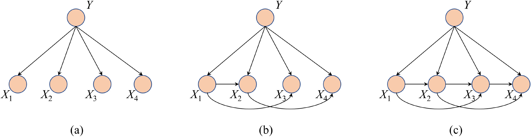$k=$ 2).

For learning BNCs from data, improving the topology of NB is an effective and efficient way to avoid the intractable complexity, and that has received great attention from researchers. An efficient machinery to manipulate and represent independence assertions is required in order to relax NB’s conditional independence assumption [5, 25]. To analyze qualitatively and measure quantitatively the mutual dependence and conditional dependence between random variables, the information-theoretic metrics, e.g., mutual information (MI) and conditional mutual information (CMI) [26], are widely applied in the learning procedure and provide a solid mathematical basis.

.

Mutual information (MI) I(X;Y) [26] measures how much information X bears on Y, and is defined as:

$\displaystyle I(X;Y)=\sum_{x\in\Omega_{X}}\sum_{y\in\Omega_{Y}}P(x,y)\log\frac% {P(x,y)}{P(x)P(y)}$ (4)

.

Conditional mutual information (CMI) $I(X_{i};X_{j}|Y)$ [26] measures the information that $X_{i}$ provides about $X_{j}$ given the value of variable $Y$ , and is defined as:

$\displaystyle I(X_{i};X_{j}|Y)=\sum_{x_{i}\in\Omega_{X_{i}}}\sum_{x_{j}\in% \Omega_{X_{j}}}\sum_{y\in\Omega_{Y}}P(x_{i},x_{j},y)\log{\displaystyle\frac{P(% x_{i},x_{j}|y)}{P(x_{i}|y)P(x_{j}|y)}}$ (5)

The absence of any conditional dependencies makes NB achieve high bias and low variance, whereas the full representation of all dependency relationships makes full BNC achieve low bias and high variance. To achieve the bias/variance trade-off, researchers propose to mine only the most significant dependency relationships implicated in data. The final probabilistic topology can be regarded as a spectrum of allowable dependence standing between NB and full BNC. Friedman [5] proposes tree-augmented naive Bayes (TAN) which learns one-dependence relationships by building a maximal weighted spanning tree [27]. By assuming that each predictive attribute can have at most $k$ other attributes as its parents, Sahami proposes $k$ -dependence Bayesian classifier (KDB) [28] which further extends NB’s topology [29]. Examples of TAN and KDB are respectively shown in Fig. 1(b) and Fig. 1(c). With more augmented arcs added to the network topology of NB, the independence assumption can be alleviated to certain extents and that is expected to help reduce bias.

2.2 Instance learning

The vast majority of learning algorithms in statistics and machine learning assume that random variables or attributes follow the i.i.d. assumption [8]. The independence assumption of the i.i.d. assumption assumes that the samples are independent from the rest of them. Similarly, the identical distribution assumption posits the underlying distribution of each random variable or attribute is the same for all samples. The i.i.d. assumption is considered to be the foundation of model selection techniques such as cross-validation and bootstrapping in statistics and machine learning. Whereas, the i.i.d. assumption is too tight for many applications [9].

BNCs represent the dependency relationships among a set of domain attributes in the form of DAG, and ideally the conditional probability distributions encoded in the DAG can fit data well. However, the real-world data generating mechanisms mostly involve various heterogeneous entities with complex relationships. To guarantee high-confidence estimates of probability distributions, commonly the DAG only describes the most significant dependency relationships implicated in the relational data while the number of instances for training is limited. Different kinds of conditional independence assertions are proposed to simplify the topology of DAG, and that may bias the estimates of conditional probability distributions. Thus the identically distributed assumption is not appropriate for precisely learning BNC from data. Take dataset segment from the UCI machine learning repository [30] as an example. Suppose that segment consists of $N$ instances and each instance appears only once, i.e., the joint probability distribution for each instance is $1/N$ . As shown in Fig. 2, the values of joint probability distribution vary greatly for different instances according to the DAGs of NB and KDB (with $k=2$ ). Thus the significance of (conditional) dependence or independence also varies greatly for different instances.

Figure 2.

The values of joint probability distribution on dataset segment for (a) NB and (b) KDB.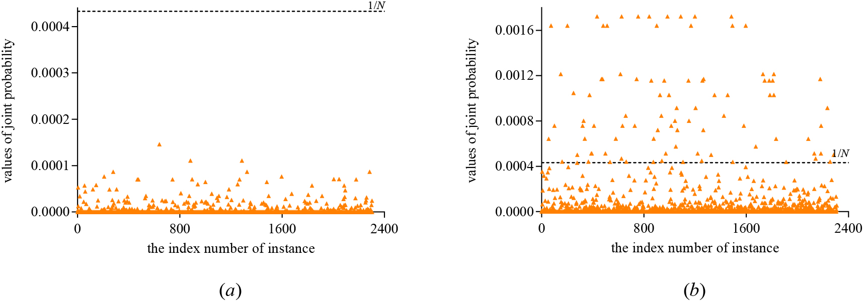

To address this issue, instance learning takes specific unlabeled instance or selected instances as the objective and learns the dependency relationships among attribute values [31]. Among instance-based learners, nearest neighbour algorithms [32] are supposed to be the simplest one. By applying domain specific distance function to learn the similarity among instances from training data, they assign the class label of the retrieved instance to the new instance. $k$ -nearest neighbour algorithms retrieve the $k$ nearest neighbours of the new instance, then select the class label which is predominant and assign it to the new instance. When $k=1$ , $k$ -nearest neighbour classifier is reduced to standard nearest neighbour classifier. Tsymbal et al. propose the K-star [33] instance-based learner which utilizes an entropy-based distance function. Jiang and Zhang [34] propose to clone training instances which are similar to the testing ones, and the expanded training data are applied to build AODE. Duan et al. [35] apply variants of information-theoretic metric as instance-based weighting function and flexibly assign distinct weights to different committee members in AODE. Zhang et al. [36] propose to combine attribute weighting with instance weighting into one uniform framework.

2.3 Multistage classification

One single BNC can represent limited number of dependency relationships and the estimate of joint probability may be biased. In contrast if the BNCs are combined as multistage classifier or ensemble, the dependency relationships may be fully represented and that will help calibrate the estimate of joint probability [37, 38]. Multistage classifier means a sequence of binary classifiers, guiding from the rough information about examined object at the early stages to the more detailed classification at the end. Silla and Freitas [39] empirically prove that adopting multistage or hierarchical classification methods to different application domains can decrease the misclassification rate. Multistage classification has been widely adopted in numerous pattern recognition fields, e.g., face recognition [40], age estimation [41], character recognition [42], and emotion recognition [43]. To overcome the weakness of Euclidean norm-based measure and improve the global recognition rates while dealing with noisy images, Grossi et al. [40] build up a cascading three-stage voting system based on the sparsity promotion worked out on the multi-feature dictionaries. For human age estimation, Liu et al. [41] also propose a three-stage learning, including age grouping, age estimation within age groups and decision fusion for final age estimation. Basu et al. [42] present a two-stage classifier which performs a coarse classification on the input pattern and then refines its earlier decision by selecting the true class from the group of candidate classes selected before. Poorna et al. [43] adopt multistage classification methodology to develop a speech emotion recognition algorithm based on Arabic speaking community.

Single-topology BNC, e.g., NB, TAN and KDB, represents the attribute dependencies over the entire dataset with one network topology. In contrast, Bayesian multinets (BMs), which are introduced in [44] and then studied in [5], compose of a series of local networks. Similar to the basic idea of clustering, an algorithm can assemble observations into groups which prior misconceptions and ignorance would otherwise preclude. To represent an asymmetric set of dependency relations between attributes, the whole dataset is partitioned into subsets according to the class labels, then each local network of BM is built on different subset. Alternatively, arbitrary partitions can be obtained, in which each partition has consistent dependency relations between attributes given the data subset which is in the partition. Therefore, more effective local BNCs can be built according to each data subset.

Figure 3.

The topologies learned from a) dataset iris, b) subset with class label 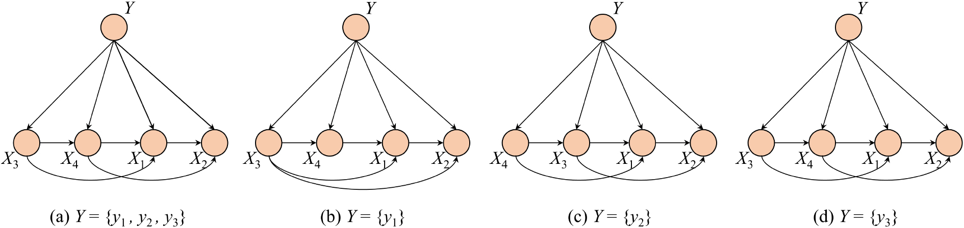$y_{1}$ , c) subset with class label $y_{2}$ and d) subset with class label $y_{3}$ .

A BMC (Bayesian multinet classifier) consists of a prior probability distribution about the class and a series of local BNCs. Each local BNC corresponds to a label that the class variable can take. Figure 3 shows the topologies of BNCs respectively learned from dataset iris and partitioned subset $\mathcal{D}_{i}(1\leqslant i\leqslant 3)$ for class label $y_{i}$ . The distinct (in)dependency relationships implicated in subset $\mathcal{D}_{1}$ are overwhelmed by those implicated in $\mathcal{D}_{2}$ and $\mathcal{D}_{3}$ , and they are not represented in the final topology. Formally, a BMC is a tuple $\mathcal{M}=<P_{Y},\mathcal{B}^{1},\dots,\mathcal{B}^{m}>$ , where $\mathcal{B}^{i}$ is the i-th local BNC corresponding to class label $y_{i}$ and $P_{Y}$ describes the priori probability distribution of class $Y$ . Diverse local BNCs with different topologies, which are learned from different data subsets, make it possible to represent asymmetric independence assertions. For the local BMC, the joint probability distribution corresponding to class label $y$ can be estimated by

$\displaystyle P(\textit{{x}}|\mathcal{B}^{y})=\prod_{i=1}^{n}P(x_{i}|\pi_{i},% \mathcal{B}^{y})$ (6)

where $\pi_{i}$ denotes the values of the parent attributes of node $X_{i}$ in $\mathcal{B}^{y}$ .

Different from the single-topology BNCs which have fixed dependency relations between attributes over all class labels, BMC allows diverse dependency relationships between the attributes for different class labels. A BMC can simulate single-topology BNC if there exists the same topology for all the local networks. The class variable in a BMC can be considered as a parent of all the attributes, and takes only one label in each local network. For example, the Bayesian Chow-Liu tree multinet classifier [45] builds each local BNC by adopting the Chow-Liu tree.

3. Algorithm

3.1 Asymmetric independence and symmetric independence

The independence assertions encoded in BNCs are likely to speed up knowledge acquisition or facilitate inference, whereas the significance of independence may vary from instance to instance.

.

[ 44 ] ${\bm{X}}_{1}$ , ${\bm{X}}_{2}$ , and ${\bm{Y}}$ are three disjoint subsets of random variables. If ${\bm{X}}_{1}$ is conditionally independent of ${\bm{X}}_{2}$ given ${\bm{Y}}$ , denoted as $I({\bm{X}}_{1}\bot{\bm{X}}_{2}|{\bm{Y}})$ , for every respective values of ${\bm{X}}_{1}$ , ${\bm{X}}_{2}$ , and ${\bm{Y}}$ , then $I({\bm{X}}_{1}\bot{\bm{X}}_{2}|\textbf{Y})$ is called symmetric independence assertion.

.

[ 44 ] If $I({\bm{X}}_{1}\bot{\bm{X}}_{2}|{\bm{Y}})$ holds for some rather than all the possible values that ${\bm{X}}_{1}$ , ${\bm{X}}_{2}$ , and ${\bm{Y}}$ can take, then $I({\bm{X}}_{1}\bot{\bm{X}}_{2}|{\bm{Y}})$ is called asymmetric independence assertion.

Asymmetric independence corresponds to asymmetries within decision trees, and asymmetric independence assertion is adapted from literatures over decision analysis [44]. Although researchers propose to extend traditional approaches considerably and make the topology of BNCs more expressive, the asymmetric independence assertions cannot be naturally represented. The formulas of traditional information-theoretic metrics (e.g., MI and CMI) consider all the possible combinations of attribute values and when applied to identify significant dependence or independence, the topology of learned BNC will remain the same while dealing with different instances.

BMCs provide an effective and feasible solution to address this issue. If the dataset $\mathcal{D}$ is partitioned into subsets $\mathcal{D}_{i}(1\leqslant i\leqslant m)$ and each of which corresponds to one distinct value of variable $Y$ , then the local BNC learned from $\mathcal{D}_{i}(1\leqslant i\leqslant m)$ can describe a joint probability of all the attributes conditioned on $y_{i}$ . All of the partitions are usually singletons, thus the asymmetric independence assertions within each local topology of BNC can be alleviated to certain extents. The independence assertions conditioned on different class labels can be fully mined.

Figure 4.

The probability that KDB can assign the right class label with different values of 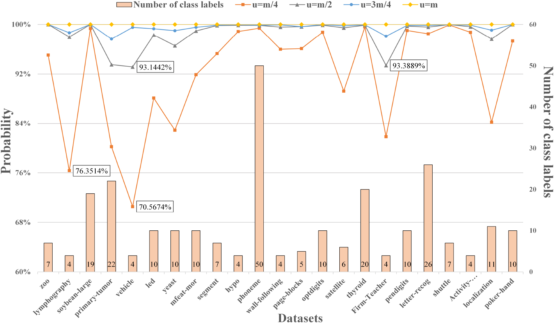$u$ as the threshold.

The confidence levels of different local BNCs will not be the same especially when dealing with unbalanced datasets. If these BNCs are treated equally then the estimate of joint probability conditioned on true class label may be overwhelmed by those conditioned on wrong class labels. As the number of class labels increases, the BNC needs to satisfy more independence assertions. Then it is possible to learn a sub-optimal BNC, and that may result in poorer classification performance. If we assign class label to testing instance ${\bm{x}}$ according to Eq. (1) and there exist high-confidence class labels for which the posterior probabilities are close to the maximum one, e.g., $c_{1}=\arg\max P({\bm{x}},c_{i})$ and $P({\bm{x}},c_{1})\approx P({\bm{x}},c_{2})$ , then choosing $c_{1}$ as the final decision is error-prone. Parameter $u$ is introduced as the confidence threshold to differentiate high-confidence class labels from low-confidence ones, and is defined as the number of class labels corresponding to the first $u$ largest joint probabilities. On the basis of this, the asymmetric independence assertions can be studied in terms of instance learning. The unlabeled instance ${\bm{x}}$ may take any one of the $m$ possible values of variable $Y$ . Thus ${\bm{x}}$ can be described in the form of pseudo training set $\mathcal{P}$ that consists of $m$ instances as Eq. (7) shows. $\mathcal{P}_{i}$ in $\mathcal{P}$ is a distinct instance with class label $y_{i}$ , and the local BNC learned from $\mathcal{P}_{i}(1\leqslant i\leqslant m)$ can describe the joint probability of all the attribute values in ${\bm{x}}$ conditioned on $y_{i}$ . Furthermore, parameter $u$ is also needed to filter out low-confidence class labels and then reduce the number of $\mathcal{P}_{i}$ for training.

$\displaystyle{\bm{x}}=\{x_{1},x_{2},\ldots,x_{n}\}\Leftrightarrow\mathcal{P}=% \left\{\begin{array}[]{l}\par \mathcal{P}_{1}=\{x_{1},x_{2},\ldots,x_{n},y_{1}% \}\\ \par \mathcal{P}_{2}=\{x_{1},x_{2},\ldots,x_{n},y_{2}\}\\ \par \cdots\\ \par \mathcal{P}_{m}=\{x_{1},x_{2},\ldots,x_{n},y_{m}\}\\ \end{array}\right.$ (7)

One class label corresponds to two local BNCs, one BNC learned from $\mathcal{D}_{i}$ and another learned from $\mathcal{P}_{i}$ . The computational overhead will increase as the number of class labels increases. Furthermore, if all the class labels are introduced to learn local BNCs, too many non-significant dependency relationships in local BNCs may result in overfitting. Thus we need to set a threshold to determine the maximum number of class labels for training. In the following discussion we take KDB with $k=2$ as the benchmark BNC to study asymmetric independence assertions, and 23 UCI datasets with more than 3 class labels are introduced for experimental study. Given different values of $u$ , the probabilities that KDB can assign the right class label are shown in Fig. 4. From Fig. 4 we can see that as $u$ increases from $\frac{m}{4}$ to $m$ , the probability also increases, and KDB performs almost the same when $u=\frac{3m}{4}$ or $u=m$ in most cases. Thus in this paper the setting $u=\frac{3m}{4}$ is selected.

3.2 Information-theoretic metric for learning local BNCs

Single-topology BNC roughly describes the dependency relationships between attributes due to the asymmetric independence assertions. One feasible solution is to precisely identify the (conditional) independence conditioned on specific class label. Suppose that for testing instance ${\bm{x}}$ , $\Omega_{Y|{\bm{x}}}$ is a set of $u$ high-confidence class labels whose posterior probabilities are close to the maximum. Those low-confidence class labels will be excluded from the formula of information-theoretic metrics, and that may help differentiate significant dependencies. Only the class labels in $\Omega_{Y|{\bm{x}}}$ will be introduced into the learning procedure of BMC.

The training data $\mathcal{D}$ is partitioned into $m$ subsets, and the instances in the subset $\mathcal{D}_{i}(1\leqslant i\leqslant m)$ have the same class label $y_{i}$ . Then CMI and MI will be respectively generalized to Class-CMI and Class-MI as follows:

$\displaystyle I(X_{i};X_{j}|y)=\sum_{x_{i}\in\Omega_{X_{i}}}\sum_{x_{j}\in% \Omega_{X_{j}}}P(x_{i},x_{j},y)\log\frac{P(x_{i},x_{j}|y)}{P(x_{i}|y)P(x_{j}|y)}$

(8) $\displaystyle\hskip 56.905512pt=P(y)\sum_{x_{i}\in\Omega_{X_{i}}}\sum_{x_{j}% \in\Omega_{X_{j}}}P(x_{i},x_{j}|y)\log\frac{P(x_{i},x_{j}|y)}{P(x_{i}|y)P(x_{j% }|y)}$ $\displaystyle I(X_{i};y)=\sum_{x_{i}\in\Omega_{X_{i}}}P(x_{i},y)\log\frac{P(x_% {i},y)}{P(x_{i})P(y)}$ (9) $\displaystyle\hskip 42.679134pt=P(y)\sum_{x_{i}\in\Omega_{X_{i}}}P(x_{i}|y)% \log\frac{P(x_{i},y)}{P(x_{i})P(y)}$

$P(y)$ in Eqs (3.2) and (3.2) is a constant for the subset with class label $y$ . To improve the generalization performance of the BNC learned from training data and address the issue of asymmetric independence assertion, BMC represents the dependency relationships implicated in specific instance based on instance learning. For instance $\mathcal{P}_{i}(1\leqslant i\leqslant m)$ in Eq. (7), CMI is generalized to point-wise Micro-CMI which measures the conditional dependence between attribute values conditioned on class label $y$ ,

$\displaystyle I(x_{i};x_{j}|y)=P(x_{i},x_{j},y)\log\frac{P(x_{i},x_{j}|y)}{P(x% _{i}|y)P(x_{j}|y)}=P(y)P(x_{i},x_{j}|y)\log\frac{P(x_{i},x_{j}|y)}{P(x_{i}|y)P% (x_{j}|y)}$ (10)

Similarly, to measure the mutual dependence between attribute value and class label $y$ we can also generalize MI to instance-based Micro-MI as follows,

$\displaystyle I(x_{i};y)=P(x_{i},y)\log\frac{P(x_{i}|y)}{P(x_{i})P(y)}=P(y)P(x% _{i}|y)\log\frac{P(x_{i}|y)}{P(x_{i})P(y)}$ (11)

$P(y)$ in Eqs (10) and (11) is also a constant for any instance in $\mathcal{P}$ . Similar to subset $\mathcal{D}_{i}$ , each pseudo instance $\mathcal{P}_{i}$ constitutes a pseudo training subset. In other words, training set $\mathcal{D}$ and pseudo training set $\mathcal{P}$ are respectively partitioned into $m$ data subsets and $m$ instantiated subsets. We can obtain the corresponding prior and joint probabilities through the subset $\mathcal{D}_{i}$ as follows,

$\displaystyle\left\{\begin{array}[]{l}\par \hat{P}(y)={\displaystyle\frac{1}{|% \mathcal{D}_{i}|}}\sum_{r=1}^{|\mathcal{D}_{i}|}\delta_{r}(y)\\ \par \hat{P}(x_{i})={\displaystyle\frac{1}{|\mathcal{D}_{i}|}}\sum_{r=1}^{|% \mathcal{D}_{i}|}\delta_{r}(x_{i})\\ \par \hat{P}(x_{i},y)={\displaystyle\frac{1}{|\mathcal{D}_{i}|}}\sum_{r=1}^{|% \mathcal{D}_{i}|}\delta_{r}(x_{i},y)\\ \par \hat{P}(x_{i},x_{j},y)={\displaystyle\frac{1}{|\mathcal{D}_{i}|}}\sum_{r=% 1}^{|\mathcal{D}_{i}|}\delta_{r}(x_{i},x_{j},y)\\ \end{array}\right.$ (12)

where $\delta_{r}(\cdot)$ is a binary function, and $\delta_{r}(\cdot)=1$ if its parameters appear in the $r$ -th instance or $\delta_{r}(\cdot)=0$ otherwise, $|\mathcal{D}_{i}|$ denotes the size of dataset $\mathcal{D}_{i}$ . Based on Bayes’ theorem, we can estimate the conditional probabilities as follows,

$\displaystyle\left\{\begin{array}[]{l}\hat{P}(x_{i}|y)={\displaystyle\frac{% \hat{P}(x_{i},y)}{\hat{P}(y)}}\\ \hat{P}(x_{i},x_{j}|y)={\displaystyle\frac{\hat{P}(x_{i},x_{j},y)}{\hat{P}(y)}% }\\ \end{array}\right.$ (13)
3.3 The three-stage classification procedure

Some state-of-the-art algorithms, e.g., TAN and KDB, learn from training dataset $\mathcal{D}$ and apply different strategies to build BNC ${}_{\mathcal{D}}$ . The topology of BNC ${}_{\mathcal{D}}$ roughly encodes the conditional dependencies between attributes whereas it cannot precisely represent the conditional dependencies between attribute values. Overfitting will make BNC ${}_{\mathcal{D}}$ closely fit the training data but perform worse on new (testing) samples. To address this issue, we propose three-stage classification for fully mining information from training data and testing data. At the pre-processing stage, benchmark BNC and local BNC ${}_{i}(1\leqslant i\leqslant m)$ are respectively learned from training dataset $\mathcal{D}$ and partitioned datasets $\mathcal{D}_{i}$ . At the learning stage, each testing instance is transformed to pseudo dataset $\mathcal{P}$ , and the low-confidence labels will be filtered out by the benchmark BNC. Then bnc ${}_{i}$ will be learned from $\mathcal{P}_{i}$ with high-confidence class label $y_{i}$ . At the classification stage, BNC ${}_{i}$ and bnc ${}_{i}(1\leqslant i\leqslant m)$ corresponding to high-confidence labels will constitute an ensemble for classification. For different testing instance, the last two stages will repeat to discriminate the asymmetric independence assertion and flexibly describe the dependency relationships implicated.

KDB controls the bias/variance trade-off by allowing each attribute to have at most $k$ parent attributes. It first collects the statistics to calculate and compare $I(X_{i};Y)$ for attribute sorting, then calculate and compare $I(X_{i};X_{j}|Y)$ , the augmented edges $X_{i}-X_{j}$ with larger value of $I(X_{i};X_{j}|Y)$ will be added to the network topolog-y. In this paper, we take KDB with $k=2$ as the benchmark BNC to learn BNC ${}_{i}$ from $\mathcal{D}_{i}$ , and the conditional dependency relationships implicated for high-confidence class label $y_{i}$ can be fully mined. The detailed learning procedure of BNC ${}_{i}$ is described by Algorithm 3.3.

[htbp] LearnStructure- $\mathcal{G}_{i}$ ( $\mathcal{D}_{i}$ , $y_{i}$ , $k$ ).Training dataset $\mathcal{D}_{i}$ , class label $y_{i}$ , and parameter $k$ . $\mathcal{G}_{i}$ , the network topology of BNC ${}_{i}$ . Calculate Class-MI $I(X_{j};y_{i})$ from $\mathcal{D}_{i}$ for all attributes. // See Eq. (3.2)Calculate Class-CMI $I(X_{j};X_{k}|y_{i})$ from $\mathcal{D}_{i}$ for each pair of attributes( $j\neq k$ ). // See Eq. (3.2)Let the selected attribute list, $\mathcal{L}$ , be empty.Let $\mathcal{G}_{i}$ be a BN with a single class node, $y_{i}$ .Select attribute $X_{i}$ as the root with the largest Class-MI value, and add it to $\mathcal{L}$ ;Add a node to $\mathcal{G}_{i}$ representing $X_{root}$ and an arc from $y_{i}$ to $X_{\textit{root}}$ ; $\mathcal{L}$ contains all attributes Select the attribute $X_{\textit{max}}$ , which is not in $\mathcal{L}$ and has the largest Class-MI value;Add a node to $\mathcal{G}_{i}$ representing $X_{\textit{max}}$ ;Add an arc from $y_{i}$ to $X_{\textit{max}}$ in $\mathcal{G}_{i}$ ;Add $q=\textit{min}(|\mathcal{L}|,k)$ arcs from $q$ distinct attributes $X_{j}$ in $\mathcal{L}$ which have the largest value of Class-CMI .Add $X_{\textit{max}}$ to $\mathcal{L}$ . return $\mathcal{G}_{i}$ . [htbp] LearnStructure- $g_{i}$ ( $\mathcal{P}_{i}$ , $y_{i}$ , $k$ ).the pseudo training dataset $\mathcal{P}_{i}$ , high-confidence class label $y_{i}$ , and parameter $k$ . $g_{i}$ , the network topology of bnc ${}_{i}$ . Calculate Micro-MI $I(x_{j};y_{i})$ from $\mathcal{P}_{i}$ for all attribute values. // See Eq. (11)Calculate Micro-CMI $I(x_{j};x_{k}|y_{i})$ from $\mathcal{P}_{i}$ for each pair of attribute values( $j\neq k$ ). // See Eq. (10)Let the selected attribute value list, $\mathcal{L}$ , be empty.Let $g_{i}$ be a BN with a single class node, $y_{i}$ .Select attribute value $x_{j}$ as the root with the largest Micro-MI value, and add it to $\mathcal{L}$ ;Add a node to $g_{i}$ representing $x_{\textit{root}}$ and an arc from $y_{i}$ to $x_{\textit{root}}$ ; $\mathcal{L}$ contains all attribute values Select the attribute value $x_{\textit{max}}$ , which is not in $\mathcal{L}$ and has the largest Micro-MI value;Add a node to $g_{i}$ representing $x_{\textit{max}}$ ;Add an arc from $y_{i}$ to $x_{\textit{max}}$ in $g_{i}$ ;Add $q=min(|\mathcal{L}|,k)$ arcs from $q$ distinct attribute values $x_{k}$ in $\mathcal{L}$ which have the largest value of Micro-CMI .Add $x_{\textit{max}}$ to $\mathcal{L}$ . return $g_{i}$ .

Similarly, to learn the conditional dependency relationships implicated in $\mathcal{P}_{i}$ given high-confidence class label $y_{i}$ , we can apply the same learning strategy but different information-theoretic metrics to build bnc ${}_{i}$ . The detailed learning procedure of bnc ${}_{i}$ is described by Algorithm 3.3. By partitioning the datasets (including training dataset and pseudo training dataset) into subsets, each local BNC is able to encode class-specific dependency relations between attributes (or attribute values). The variation in dependency relationships implicated can be fully described and that can greatly help alleviate the negative effect caused by asymmetric independence assumption. In order to avoid unreliable probability estimates, when classifying an instance ${\bm{x}}$ the ensemble excludes the local BNCs which take low-confidence class labels. As discussed in Section 3.1, we set $u=3m/4$ to determine the set of high-confidence class labels. Since low-confidence class label may also be the true one for ${\bm{x}}$ , by averaging the predictions of the qualified committee members of the ensemble, the joint probability $P(y,{\bm{x}})$ for any possible class label is estimated by

$\displaystyle P_{\text{CSB}}(y,{\bm{x}})=\frac{\sum_{i:1\leqslant i\leqslant u% ∼{}\wedge∼{}y_{i}\in\Omega_{Y|{\bm{x}}}}∼{}[P(y,{\bm{x}}|\text{BNC}_{\textit{i% }})+P(\textit{y},{\bm{x}}|\text{bnc}_{\textit{i}})]}{2*|\{i:1\leqslant i% \leqslant u∼{}\wedge∼{}y_{i}\in\Omega_{Y|{\bm{x}}}\}|}$ (14)

where BNC ${}_{i}$ and bnc ${}_{i}$ respectively denote the local BNCs learned from $\mathcal{D}_{i}$ and $\mathcal{P}_{i}$ for high-confidence label $y_{i}$ .

Restricted BNCs take the class variable as the common parent of the predictive attributes, and the asymmetric independence assertions also take the class variable as a distinguished variable. The final BMC comprises several BNCs, the topology of each of them describes the joint probability for data subset where the distinguished variable (e.g., $Y$ ) takes one specific value, and the asymmetric independence assertions can be represented within each local topology [29]. Thus in this paper, to achieve the bias/variance trade-off, the dataset is partitioned into training set and pseudo training set for each testing instance. To address the issue of the asymmetric independence assertions, these two sets are further partitioned according to different class labels, and local BNCs are learned from these partitions and constitute an ensemble for classification. The learning framework of CSB is depicted in Fig. 5. The detailed learning procedure is described in Algorithm 3.3.

[htbp] Learning process of CSBTraining dataset $\mathcal{D}$ , testing dataset $\mathcal{T}$ with $M$ instances and parameter $k$ . Predicted class labels for testing instances. Pre-processing stage benchmark BNC $\leftarrow$ KDB with $k=2$ ; Partition $\mathcal{D}$ into $m$ training subsets $\mathcal{D}_{i}$ , where $i\in[1,m]$ . $y_{i}\in\Omega_{Y}$ BNC ${}_{i}\leftarrow$ LearnStructure- $\mathcal{G}_{i}(\mathcal{D}_{i},y_{i},k)$ . /*Algorithm 1*/ $j=1,\ldots,M$ x $\leftarrow$ The $j$ th instance from $\mathcal{T}$ ;

Learning stage $\Omega_{Y|\emph{{x}}}$ $\leftarrow$ $u$ high-confidence class labels for instance x learned by benchmark BNC;Transform x to pseudo training dataset $\mathcal{P}$ with $m$ pseudo instances; $y_{i}\in\Omega_{Y|\textbf{x}}$ bnc ${}_{i}\leftarrow$ LearnStructure- $g_{i}(\mathcal{P}_{i},y_{i},k)$ . /*Algorithm 2*/

Classification stage $\mathcal{B}\leftarrow\emptyset$ ; $y_{i}\in\Omega_{Y|\textbf{x}}$ $\mathcal{B}\leftarrow\mathcal{B}∼{}\cup$ BNC ${}_{i}$ $\cup$ bnc ${}_{i}$ ;return $\hat{y}\leftarrow\mathop{\textit{argmax}}\limits_{y\in\Omega_{Y}}P_{\mathcal{B% }}(y,\emph{{x}})$ ;

4. Empirical study

In this section, to evaluate the efficacy of multistage learning, we compare the performance of our proposed algorithm CSB with state-of-the-art semi-naive BNCs based on attribute selection, attribute weighting, topology extension and model selection. The $k$ value of CSB is set to 2. The detail of these BNCs for comparison study are shown as follows:

•
CFWNB [51], correlation-based attribute weighting filter for NB.

Figure 5.
The learning framework of the CSB algorithm.

•
AIWNB [36], attribute and instance weighted NB.
•
SKDB [27], selective $k$ -dependence Bayesian classifier ( $k=5$ ).
•
WATAN [25], weighted averaged tree augmented NB.
•
SA2DE [52], selective A2DE.
•
ATODE [31], averaged tree-augmented one-dependence estimators.
•
SLB [11], semi-lazy Bayesian network classifier.

The performance is analyzed in terms of zero-one loss, root mean square error (RMSE), Friedman test and Nemenyi test on 28 datasets from the UCI repository of machine learning [30]. Table 2 describes the characteristics of each dataset, including the number of instances, attributes and class labels. Table 3 presents the detailed description about the statistics we employed to interpret the results. For qualitative and quantitative attributes, the missing values are respectively replaced by modes that mostly appear or means from the training data. The minimum description length discretization method is adopted to discretize numeric attributes for each benchmark dataset [53]. 10 runs of 10-fold cross validation is used to test each algorithm on each dataset. Tables A1 and A2 in Appendix respectively present the detailed results of zero-one loss and RMSE.

Table 2
Descriptions of the UCI datasets for experimental study. Symbol “*” denotes the dataset with no less than 4 class labels

No. Dataset Instance Attribute Class

1 lung-cancer 32 56 3

2 zoo ${}^{\ast}$ 101 16 7

3 lymphography ${}^{\ast}$ 148 18 4

4 iris 150 4 3

5 soybean-large ${}^{\ast}$ 307 35 19

6 primary-tumor ${}^{\ast}$ 339 17 22

7 balance-scale 625 4 3

8 vehicle ${}^{\ast}$ 846 18 4

9 led ${}^{\ast}$ 1000 7 10

10 yeast ${}^{\ast}$ 1484 8 10

11 mfeat-mor ${}^{\ast}$ 2000 6 10

12 segment ${}^{\ast}$ 2310 19 7

13 hypo ${}^{\ast}$ 3772 29 4

14 abalone 4177 8 3

15 phoneme ${}^{\ast}$ 5438 7 50

16 wall-following ${}^{\ast}$ 5456 24 4

17 page-blocks ${}^{\ast}$ 5473 10 5

18 optdigits ${}^{\ast}$ 5620 64 10

19 satellite ${}^{\ast}$ 6435 36 6

20 thyroid ${}^{\ast}$ 9169 29 20

21 firm-Teacher ${}^{\ast}$ 10800 19 4

22 pendigits ${}^{\ast}$ 10992 16 10

23 letter-recog ${}^{\ast}$ 20000 16 26

24 shuttle ${}^{\ast}$ 58000 9 7

25 connect-4 67557 42 3

26 activity-recognition-with ${}^{\ast}$ 75128 8 4

27 localization ${}^{\ast}$ 164860 5 11

28 poker-hand ${}^{\ast}$ 1025010 10 10

Table 3
A summary table of the statistics employed

Statistics employed Description

Zero-one loss [47] Zero-one loss (ZOL) is a loss function to evaluate the classification accuracy. Let $y$ and $\hat{y}$ represent the true class label and predicting class label respectively. $\delta_{r}(y,\hat{y})=1$ if $y=\hat{y}$ and $\delta_{r}(y,\hat{y})=0$ otherwise in the $r$ -th instance. Given training data $\mathcal{D}$ with $N$ instances, the ZOL of BNC $\mathcal{B}$ is defined as follows,

$\eta(\mathcal{B})=\frac{1}{N}\displaystyle\sum_{r=1}^{N}\{1-\delta_{r}(y,\hat{% y})\}\hfill(15)$

RMSE [48] Given $N$ training instances, RMSE (root mean squared error) is defined as follows,

$\text{RMSE}=\sqrt{\displaystyle\frac{1}{N}\mathop{\sum}\limits_{i=1}^{N}(1-P(% \hat{y_{i}}|\bm{x}))^{2}}\hfill(16)$

where $\hat{y_{i}}$ represents the predicted class label in the $i$ -th instance.

Friedman [49] and Nemenyitest [50] Given $D$ datasets, the Friedman statistic is defined as follows, $F_{\rm F}=\displaystyle\frac{(D-1)\chi_{F}^{2}}{D(n-1)-\chi_{F}^{2}}\hfill(17)$ where $\chi_{F}^{2}=\displaystyle\frac{12D}{n(n+1)}\mathop{\sum}\nolimits_{i=1}^{n}R_% {i}^{2}-3D(n+1)\hfill(18)$ where $n$ denotes the number of classifiers being employed to compare and $R_{i}$ denotes the mean rank of the $i$ -th classifier.

By alleviating the asymmetric independence assumption, the topologies learned from training set or testing instance can fit data well. To prove the effectiveness of the class-specific learning mechanism, two versions of class-specific BNCs, called CSB ${}^{G}$ and CSB ${}^{L}$ , are introduced to respectively learn from partitioned training set or partitioned pseudo training set for classification. Figure 6 displays the comparison results of relative zero-one loss $\eta(A/B)=\eta(A)/\eta(B)$ , where $\eta(A)$ and $\eta(B)$ respectively denote the zero-one loss of algorithms A and B. In Fig. 6, the dotted line corresponds to $\eta(A/B)=1.0$ when both of the algorithms perform almost the same. From Figs 6(a) and 6(b) we can see that the data points appear below the dotted line much more often than not, that means both CSB ${}^{L}$ and CSB ${}^{G}$ significantly help improve the zero-one loss of KDB with $k=2$ . Furthermore, as shown in Figs 6(c) and 6(d), the comparison results indicate that CSB outperforms CSB ${}^{L}$ and CSB ${}^{G}$ on zero-one loss, thus CSB inherits the advantages of both CSB ${}^{L}$ and CSB ${}^{G}$ and achieves better performance.

Figure 6.
The comparison results of relative zero-one loss. The X-axis presents the index number of datasets, Y-axis presents 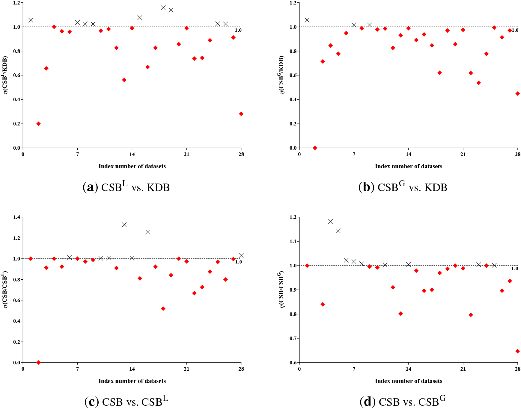$\eta(A/B)=\eta(A)/\eta(B)$ for the compared classifiers A and B, and each point corresponds to one dataset.

4.1 Comparison study in terms of zero-one loss and RMSE

No.	Dataset	Instance	Attribute	Class
1	lung-cancer	32	56	3
2	zoo ${}^{\ast}$	101	16	7
3	lymphography ${}^{\ast}$	148	18	4
4	iris	150	4	3
5	soybean-large ${}^{\ast}$	307	35	19
6	primary-tumor ${}^{\ast}$	339	17	22
7	balance-scale	625	4	3
8	vehicle ${}^{\ast}$	846	18	4
9	led ${}^{\ast}$	1000	7	10
10	yeast ${}^{\ast}$	1484	8	10
11	mfeat-mor ${}^{\ast}$	2000	6	10
12	segment ${}^{\ast}$	2310	19	7
13	hypo ${}^{\ast}$	3772	29	4
14	abalone	4177	8	3
15	phoneme ${}^{\ast}$	5438	7	50
16	wall-following ${}^{\ast}$	5456	24	4
17	page-blocks ${}^{\ast}$	5473	10	5
18	optdigits ${}^{\ast}$	5620	64	10
19	satellite ${}^{\ast}$	6435	36	6
20	thyroid ${}^{\ast}$	9169	29	20
21	firm-Teacher ${}^{\ast}$	10800	19	4
22	pendigits ${}^{\ast}$	10992	16	10
23	letter-recog ${}^{\ast}$	20000	16	26
24	shuttle ${}^{\ast}$	58000	9	7
25	connect-4	67557	42	3
26	activity-recognition-with ${}^{\ast}$	75128	8	4
27	localization ${}^{\ast}$	164860	5	11
28	poker-hand ${}^{\ast}$	1025010	10	10

Statistics employed	Description
Zero-one loss [47]	Zero-one loss (ZOL) is a loss function to evaluate the classification accuracy. Let $y$ and $\hat{y}$ represent the true class label and predicting class label respectively. $\delta_{r}(y,\hat{y})=1$ if $y=\hat{y}$ and $\delta_{r}(y,\hat{y})=0$ otherwise in the $r$ -th instance. Given training data $\mathcal{D}$ with $N$ instances, the ZOL of BNC $\mathcal{B}$ is defined as follows,
	$\eta(\mathcal{B})=\frac{1}{N}\displaystyle\sum_{r=1}^{N}\{1-\delta_{r}(y,\hat{% y})\}\hfill(15)$
RMSE [48]	Given $N$ training instances, RMSE (root mean squared error) is defined as follows,
	$\text{RMSE}=\sqrt{\displaystyle\frac{1}{N}\mathop{\sum}\limits_{i=1}^{N}(1-P(% \hat{y_{i}}\|\bm{x}))^{2}}\hfill(16)$
	where $\hat{y_{i}}$ represents the predicted class label in the $i$ -th instance.
Friedman [49] and Nemenyitest [50]	Given $D$ datasets, the Friedman statistic is defined as follows, $F_{\rm F}=\displaystyle\frac{(D-1)\chi_{F}^{2}}{D(n-1)-\chi_{F}^{2}}\hfill(17)$ where $\chi_{F}^{2}=\displaystyle\frac{12D}{n(n+1)}\mathop{\sum}\nolimits_{i=1}^{n}R_% {i}^{2}-3D(n+1)\hfill(18)$ where $n$ denotes the number of classifiers being employed to compare and $R_{i}$ denotes the mean rank of the $i$ -th classifier.

To prove the effectiveness of CSB, the BNCs for comparison study are divided into two groups: single-topology BNCs (including CFWNB, AIWNB and SKDB) and ensemble BNCs (including WATAN, SA2DE, ATODE and SLB). One-tailed $t$ -test with significance level $p=0.05$ is introduced for pair-wise comparison. The comparison results of zero-one loss are listed in Table 4 in the form of $i(j)$ , where $i$ denotes the number of datasets on which the algorithm in the column performs better than the one in the corresponding row, and $j$ is the number of datasets on which the algorithm performs significantly better with significance level $p=0.05$ .

Table 4
The compared results of the corrected paired one-tailed $t$ -test ( $p=0.05$ ) on zero-one loss

	CFWNB	AIWNB	SKDB	WATAN	SA2DE	ATODE	SLB	CSB
CFWNB	–	20 (14)	17 (14)	20 (15)	23 (18)	20 (18)	22 (19)	24 (19)
AIWNB	6 (3)	–	14 (13)	19 (14)	17 (14)	18 (16)	19 (16)	22 (19)
SKDB	10 (6)	13 (8)	–	16 (13)	18 (9)	20 (12)	23 (17)	22 (16)
WATAN	8 (5)	9 (8)	12 (10)	–	12 (10)	17 (13)	21 (17)	23 (18)
SA2DE	5 (5)	10 (8)	10 (8)	15 (7)	–	15 (11)	21 (15)	20 (18)
ATODE	8 (3)	10 (5)	7 (7)	10 (3)	13 (7)	–	18 (14)	20 (15)
SLB	6 (2)	8 (5)	5 (5)	5 (1)	5 (3)	9 (4)	–	17 (11)
CSB	4 (3)	6 (3)	5 (4)	5 (1)	7 (2)	6 (2)	10 (4)	–

Table 5

The comparison results of the corrected paired one-tailed $t$ -test ( $p=0.05$ ) on RMSE

	CFWNB	AIWNB	SKDB	WATAN	SA2DE	ATODE	SLB	CSB
CFWNB	–	24 (12)	17 (15)	21 (17)	21 (19)	22 (20)	23 (20)	24 (21)
AIWNB	3 (3)	–	15 (12)	18 (16)	19 (16)	20 (16)	20 (16)	25 (20)
SKDB	11 (6)	13 (7)	–	16 (9)	19 (7)	29 (12)	20 (16)	23 (14)
WATAN	7 (4)	10 (7)	12 (8)	–	12 (7)	20 (11)	22 (14)	22 (16)
SA2DE	7 (5)	9 (6)	9 (7)	16 (7)	–	18 (9)	20 (13)	23 (15)
ATODE	6 (3)	8 (4)	9 (7)	8 (3)	10 (3)	–	18 (7)	19 (12)
SLB	5 (3)	8 (4)	8 (6)	6 (1)	(5)	7 (3)	–	17 (8)
CSB	4 (1)	3 (1)	5 (4)	6 (1)	4 (1)	9 (1)	11 (3)	–

From Table 4 we can see that, for single-topology BNCs structure extension is more effective compared to attribute weighting. For CFWNB, each attribute weight is a sigmoid transformation of the difference between the average attribute-attribute intercorrelation (average mutual redundancy) and the attribute-class correlation (mutual relevance). AIWNB utilizes a lazy approach to learning instance weights and a correlation-based attribute weighting approach to learning attribute weights, in which instance weighting and attribute weighting are combined into one uniform framework. SKDB, which relaxes NB’s independence assumption by adding augmented edges, selects appropriate parameter $k$ by applying leave-one-out cross validation. CSB performs the best with respect to zero-one loss, followed by SKDB, and it respectively beats SKDB, CFWNB and AIWNB on 16, 19 and 19 datasets, and loses on 4, 3 and 3 datasets.

Ensemble learning can represent more dependency relationships than single-topology BNCs and the topology of each committee member can be relatively simpler. The experimental results indicate that all the ensemble classifiers can achieve better performance than single-topology BNCs (e.g., CFWNB, AIWNB and SKDB). The TAN members of WATAN share the same topology skeleton but have different directed edges, the weighting metrics can tune the estimates of joint probabilities for different TAN members. SA2DE can represent high-dependence relationships and only high-confidence members are selected for prediction. ATODE conducts topology augmentation by applying log likelihood function to identify significant dependency relations. SLB learns class-specific BNCs to mine the dependency relations hidden in attribute values of testing instance with a supposed class label. Experimental results show that our multistage classification strategy provides low zero-one loss or high classification accuracy. As shown in Table 4, CSB performs significantly better than WATAN, SA2DE, ATODE and SLB on 18, 18, 15, 11 datasets, respectively. According to the experimental results, we can argue that CSB provides a more effective ensemble of class-specific BNCs with respect to zero-one loss.

Table 5 presents the experimental results in terms of RMSE. Compared with lower-dependence BNCs, higher-dependence BNCs can provide more reliable estimate of conditional probability. Table 5 shows that SKDB enjoys significant advantages over CFWNB (15 wins and 6 losses) and AIWNB (12 wins and 7 losses) in terms of RMSE. Among ensemble models, CSB still performs the best. For example, CSB performs much better than WATAN (16 wins and 1 loss), SA2DE (15 wins and 1 loss) and ATODE (12 wins and 1 loss). Meanwhile, CSB also outperforms SLB (8 wins and 3 losses). The experimental results from the perspective of RMSE show that the multistage classification strategy helps CSB fit data better.

4.2 Comparison of running time

Figure 7.

Training and classification time comparisons for 8 BNCs on 28 datasets.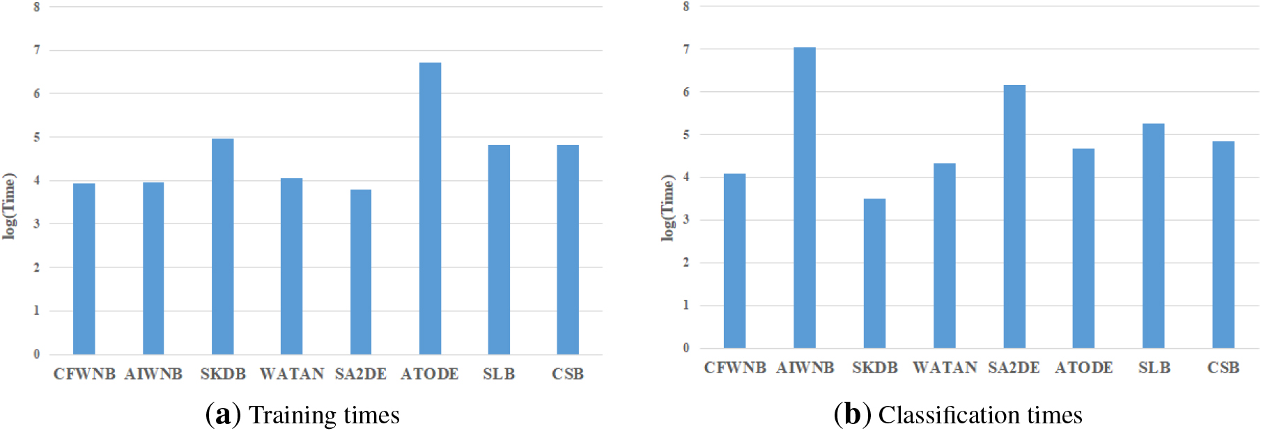

We compare the training and classification time for all the BNCs considered. The comparison results are shown in Fig. 7 and each bar denotes the averaged time on 28 datasets in a 10 runs of 10-fold cross-validation experiment. These experiments have been conducted on a desktop computer with an AMD(R) Ryzen(TM) 4600-H CPU @ 3.0 GHz, 64 bits and 16,384 MB of memory. As shown in Fig. 7(a), during the classification phase, SA2DE takes the least time and it performs attribute selection on superparents. AIWNB and CFWNB need to perform attribute weighting based on different information-theoretic metrics. WATAN needs to build a set of maximum weighted spanning trees (MWSTs) and to learn the weights for them. CSB, SLB and SKDB need more time for building high-dependence DAGs. ATODE consumes the most time because it uses log likelihood function to build high-dependence MWSTs.

During the classification phase, single BNCs, e.g., SKDB and CFWNB, consume the least time for estimating the joint probability. In contrast, ensemble BNCs, e.g., WATAN, ATODE, CSB and SLB, require more time to estimate the individual joint probability learned from each member. WATN and ATODE take different attribute as the root node of the topology in turn. CSB performs multistage classification and builds u local BNCs for high-confidence class labels. Instance learning makes the BNCs take the most time for extracting knowledge from testing instance. SLB calculates local information-theoretic metrics for different instances, SA2DE estimates the joint probability distributions through the instance with the selected attribute values, and AIWNB performs instance weighting for each instance. Although the advantages of CSB on training time and classification time are not significant, CSB can obtain significant improvement on the classification performance. Therefore, the consumption in terms of training time and classification time is perfectly acceptable.

4.3 Significance test

Figure 8.

The results of average rank in terms of zero-one loss and RMSE for alternative algorithms.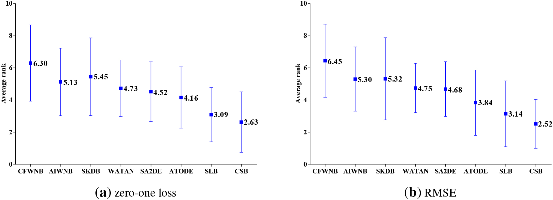

Figure 9.

The results of Nemenyi tests in terms of zero-one loss and RMSE for alternative algorithms.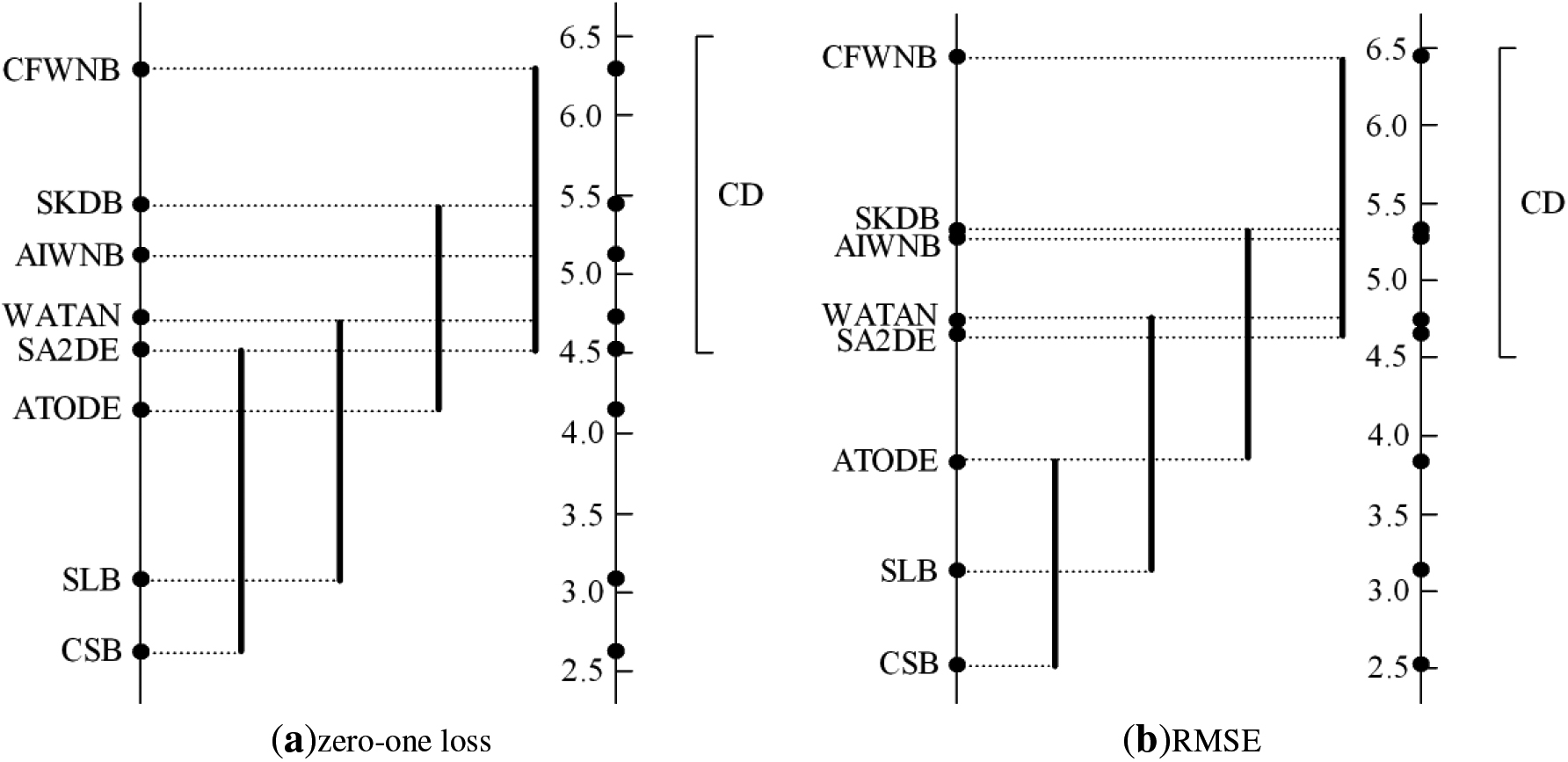

To illustrate the statistical significance of different metrics, we perform a non-parametric Friedman test followed by Nemenyi post test to statistically compare multiple algorithms on multiple datasets in terms of zero-one loss and RMSE. The Friedman test needs to rank the algorithms on each dataset, the null hypothesis of which is that all algorithms are equivalent. The detailed results of rank are presented in Tables A3 and A4 in Appendix respectively. The Friedman statistic is distributed according to $\mathcal{X}_{F}^{2}$ with $t-1$ degrees of freedom. Thereby, for any pre-determined level of significance $\alpha$ , the null hypothesis will be rejected if $\mathcal{X}_{F}^{2}>\mathcal{X}_{\alpha}^{2}$ . The critical value of $\mathcal{X}_{\alpha}^{2}$ for $\alpha=0.05$ with 7 degrees of freedom is 14.07. The Friedman statistics are 48.20 for zero-one loss and 53.39 for RMSE, both of which are greater than 14.07. Therefore, the null-hypotheses can be rejected.

The average ranks for all of the classifiers are depicted in Fig. 8, and lower rank corresponds to better classification performance. As shown in Fig. 8(a), CSB obtains the lowest average zero-one loss rank (2.63), followed by SLB (3.09), ATODE(4.16), SA2DE(4.52), WATAN(4.73), AIWNB(5.13), SKDB(5.45) and CFWNB(6.30). Obviously, our proposed CSB significantly improves upon the zero-one loss and enjoys a significant advantage relative to the other algorithms. When RMSE is compared, as shown in Fig. 8(b), CSB still gets the first position (2.52) and achieves the lowest average RMSE rank than all the other algorithms. The experimental results illustrate that our proposed multistage strategy has the greatest positive effect on reducing the RMSE.

To further explore the significant difference among these algorithms, Nemenyi test is performed and the critical value $q_{\alpha}$ for significance level $\alpha=0.05$ is 3.031. The difference in classification performance between two algorithms can be evaluated in terms of corresponding average ranks. The critical difference (CD), which is applied as the threshold for determining whether the difference is significant, is defined as follows:

$\displaystyle\textit{CD}=q_{\alpha}\sqrt{\frac{t(t+1)}{6N}}$ (19)

With 8 algorithms ( $t=8$ ) and 28 datasets ( $N=28$ ), CD $=3.031\times\sqrt{8\times(8+1)/(6\times 28)}=1.9843$ . Corresponding experimental results are shown in Fig. 9. The BNCs for comparison study and their average ranks are respectively depicted on the left line and the parallel right line. The lower position corresponds to the lower rank. The line connecting different algorithms means non-significant difference.

From Fig. 9(a) we can see that, with respect to zero-one loss, CSB performs better than SLB, ATODE and SA2DE, and its advantage over WATAN, SKDB, AIWNB and CFWNB is significant. As shown in Fig. 9(b), CSB ranks first in terms of RMSE and is followed by SLB and ATODE, in contrast its advantage over SA2DE, WATAN, AIWNB, SKDB and CFWNB is significant.

5. Conclusions and future work

The i.i.d. assumption simplifies the computational complexity while learning BNCs from datasets with complex dependencies. However, different classes of datasets may demonstrate significantly different probability distributions and thus it is hard to fully represent the dependency relationships implicated. According to the asymmetric independence assertion, in this paper we propose to partition the datasets into several subsets according to the high-confidence class labels. The BMC with two sets of class-specific BNCs can be learned from training data and testing data based on multi-stage learning, and its advantage over other single-topology BNCs and ensemble BNCs is obvious from the experimental results in terms of zero-one loss and RMSE. The Friedman test and Nemenyi test illustrate that CSB also performs the best generally. Generalized BNCs learned from labeled training data and specialized BNCs learned from unlabeled testing data contribute to the completeness of domain knowledge. In this paper we propose to apply multistage classification to build BMC, whereas these two kinds of BNCs are treated equally. The study of model weighting or model selection is needed to be introduced into the learning procedure to make these BNCs work as a whole, and we leave it to future research work.

Footnotes

Acknowledgments

This work is supported by the National Key Research and Development Program of China (No.2019YFC1804804), Open Research Project of The Hubei Key Laboratory of Intelligent Geo-Information Processing (No.KLIGIP-2021A04), and the Scientific and Technological Developing Scheme of Jilin Province (No.20200201281JC) and High Performance Computing Center of Jilin University, China.

Conflict of interest

The authors declare that they have no conflict of interest.

Appendix A

See Tables A1–A4.

Table A1

Experimental results of zero-one loss

Dataset	CFWNB	AIWNB	SKDB	WATAN	SA2DE	ATODE	SLB	CSB
Lung-cancer	0.4687	0.5000	0.5000	0.6250	0.6563	0.5313	0.6250	0.5938
Zoo	0.0396	0.0396	0.0396	0.0198	0.0297	0.0198	0.0297	0.0000
Lymphography	0.1486	0.1689	0.2770	0.1689	0.2635	0.1554	0.1554	0.1419
Iris	0.0600	0.0600	0.0867	0.0800	0.0800	0.0867	0.0800	0.0867
Soybean-large	0.0977	0.0749	0.1140	0.1010	0.1173	0.0782	0.0912	0.0782
Primary-tumor	0.5634	0.5634	0.5841	0.5428	0.5575	0.5782	0.5457	0.5546
Balance-scale	0.2496	0.2544	0.2912	0.2736	0.2800	0.2832	0.2544	0.2880
Vehicle	0.3711	0.3227	0.2920	0.2943	0.2790	0.2766	0.2896	0.2931
Led	0.2630	0.2620	0.2730	0.2660	0.2620	0.2690	0.2650	0.2650
Yeast	0.4319	0.4212	0.4461	0.4171	0.4245	0.4218	0.4239	0.4259
Mfeat-mor	0.3060	0.3050	0.3140	0.2980	0.3005	0.3105	0.2990	0.3025
Segment	0.0640	0.0472	0.0615	0.0394	0.0571	0.0346	0.0364	0.0355
Splice-c4.5	0.0374	0.0346	0.0818	0.0466	0.0337	0.0362	0.2524	0.0796
Hypo	0.0121	0.0101	0.0175	0.0130	0.0080	0.0119	0.0103	0.0085
Abalone	0.4754	0.4654	0.4680	0.4582	0.4594	0.4465	0.4503	0.4534
Phoneme	0.2407	0.2139	0.1909	0.2345	0.1824	0.2427	0.2464	0.1730
Wall-following	0.0720	0.0378	0.0286	0.0550	0.0442	0.0361	0.0480	0.0337
Page-blocks	0.0416	0.0353	0.0331	0.0418	0.0358	0.0327	0.0312	0.0298
Optdigits	0.0676	0.0628	0.0641	0.0406	0.0404	0.0290	0.0246	0.0224
Satellite	0.1726	0.1434	0.1206	0.1207	0.1276	0.1147	0.1086	0.1033
Thyroid	0.0817	0.1030	0.0784	0.0723	0.0605	0.0629	0.0101	0.0605
Firm-Teacher	0.2359	0.2324	0.1779	0.1934	0.1985	0.2125	0.1737	0.1749
Pendigits	0.1129	0.0635	0.0794	0.0328	0.0491	0.0200	0.0189	0.0145
Letter-recog	0.2479	0.2041	0.1177	0.1300	0.0769	0.0838	0.0625	0.0532
Shuttle	0.0020	0.0016	0.0009	0.0014	0.0017	0.0008	0.0006	0.0007
Connect-4	0.2847	0.2827	0.2007	0.2354	0.2397	0.2374	0.2343	0.2271
Activity-recognition-with	0.0429	0.0384	0.0183	0.0179	0.0168	0.0174	0.0132	0.0104
Waveform	0.0198	0.0196	0.0285	0.0202	0.1662	0.0182	0.1720	0.1688
Localization	0.4936	0.4643	0.3013	0.3575	0.3078	0.3544	0.2708	0.2694
Poker-hand	0.4988	0.4988	0.0318	0.3295	0.1967	0.3453	0.0792	0.0569

The value in boldface indicates the classifier with the best performance.

Table A2

Experimental results of RMSE

Dataset	CFWNB	AIWNB	SKDB	WATAN	SA2DE	ATODE	SLB	CSB
Lung-cancer	0.4814	0.5287	0.5121	0.6218	0.5892	0.5692	0.6241	0.5005
Zoo	0.0933	0.0883	0.0884	0.0614	0.0746	0.0686	0.0640	0.0605
Lymphography	0.2419	0.2591	0.3156	0.2705	0.3027	0.2501	0.2645	0.2528
Iris	0.1500	0.1499	0.1970	0.1958	0.2063	0.2077	0.1999	0.1948
Soybean-large	0.0886	0.0809	0.0978	0.0902	0.0962	0.0856	0.0833	0.0774
Primary-tumor	0.1790	0.1782	0.1917	0.1812	0.1823	0.1864	0.1770	0.1772
Balance-scale	0.3589	0.3507	0.3127	0.3203	0.3206	0.3198	0.3153	0.3252
Vehicle	0.3611	0.3288	0.3233	0.3103	0.3116	0.3083	0.3060	0.3101
Led	0.2163	0.2130	0.2023	0.1991	0.1986	0.1980	0.1990	0.1986
Yeast	0.2423	0.2404	0.2440	0.2376	0.2377	0.2371	0.2371	0.2372
Mfeat-mor	0.1943	0.1927	0.2003	0.1941	0.1966	0.1980	0.1966	0.1950
Segment	0.1195	0.1029	0.1210	0.0968	0.1081	0.0881	0.0917	0.0874
Splice-c4.5	0.1388	0.1337	0.2149	0.1541	0.1337	0.1366	0.3681	0.2534
Hypo	0.0739	0.0661	0.0840	0.0723	0.0596	0.0685	0.0685	0.0593
Abalone	0.4433	0.4337	0.4449	0.4250	0.4220	0.4195	0.4243	0.4358
Phoneme	0.0806	0.0776	0.0756	0.0844	0.0737	0.0891	0.0848	0.0727
Wall-following	0.1744	0.1295	0.1088	0.1570	0.1368	0.1298	0.1483	0.1159
Page-blocks	0.1117	0.1044	0.1064	0.1187	0.1040	0.1013	0.0998	0.0975
Optdigits	0.1075	0.1019	0.1035	0.0835	0.0829	0.0727	0.0643	0.0984
Satellite	0.2316	0.2061	0.1917	0.1849	0.1862	0.1799	0.1752	0.1628
Thyroid	0.0789	0.0905	0.0813	0.0742	0.1815	0.0706	0.0677	0.0675
Firm-Teacher	0.3177	0.3138	0.2520	0.2706	0.2711	0.2809	0.2895	0.2712
Pendigits	0.1318	0.0979	0.1128	0.0725	0.0899	0.0565	0.0544	0.0593
Letter-recog	0.1139	0.1036	0.0823	0.0859	0.0670	0.0691	0.0596	0.0645
Shuttle	0.0270	0.0220	0.0143	0.0177	0.0181	0.0124	0.0124	0.0129
Connect-4	0.3632	0.3620	0.3062	0.3315	0.3349	0.3339	0.3299	0.3337
Activity-recognition-with	0.1246	0.1188	0.0835	0.0845	0.0822	0.0832	0.0720	0.0687
Waveform	0.1116	0.1079	0.1087	0.0951	0.2778	0.0865	0.0974	0.0900
Localization	0.2402	0.2351	0.2010	0.2095	0.2000	0.2081	0.1848	0.1844
Poker-hand	0.2382	0.2382	0.0748	0.2124	0.1770	0.2153	0.1566	0.1574

The value in boldface indicates the classifier with the best performance.

Table A3

Experimental results of rank in terms of zero-one loss

Dataset	CFWNB	AIWNB	SKDB	WATAN	SA2DE	ATODE	SLB	CSB
Lung-cancer	1.0	2.5	2.5	6.5	8.0	4.0	6.5	5.0
Zoo	7.0	7.0	7.0	2.5	4.5	2.5	4.5	1.0
lymphography	2.0	5.5	8.0	5.5	7.0	3.5	3.5	1.0
Iris	1.5	1.5	7.0	4.0	4.0	7.0	4.0	7.0
soybean-large	5.0	1.0	7.0	6.0	8.0	2.5	4.0	2.5
Primary-tumor	5.5	5.5	8.0	1.0	4.0	7.0	2.0	3.0
Balance-scale	1.0	2.5	8.0	4.0	5.0	6.0	2.5	7.0
Vehicle	8.0	7.0	4.0	6.0	2.0	1.0	3.0	5.0
Led	3.0	1.5	8.0	6.0	1.5	7.0	4.5	4.5
Yeast	7.0	2.0	8.0	1.0	5.0	3.0	4.0	6.0
Mfeat-mor	6.0	5.0	8.0	1.0	3.0	7.0	2.0	4.0
Segment	8.0	5.0	7.0	4.0	6.0	1.0	3.0	2.0
Splice-c4.5	4.0	2.0	7.0	5.0	1.0	3.0	8.0	6.0
Hypo	6.0	3.0	8.0	7.0	1.0	5.0	4.0	2.0
Abalone	8.0	6.0	7.0	4.0	5.0	1.0	2.0	3.0
Phoneme	6.0	4.0	3.0	5.0	2.0	7.0	8.0	1.0
Wall-following	8.0	4.0	1.0	7.0	5.0	3.0	6.0	2.0
Page-blocks	7.0	5.0	4.0	8.0	6.0	3.0	2.0	1.0
Optdigits	8.0	6.0	7.0	5.0	4.0	3.0	2.0	1.0
Satellite	8.0	7.0	4.0	5.0	6.0	3.0	2.0	1.0
Thyroid	7.0	8.0	6.0	5.0	2.5	4.0	1.0	2.5
Firm-Teacher	8.0	7.0	3.0	4.0	5.0	6.0	1.0	2.0
Pendigits	8.0	6.0	7.0	4.0	5.0	3.0	2.0	1.0
Letter-recog	8.0	7.0	5.0	6.0	3.0	4.0	2.0	1.0
Shuttle	8.0	6.0	4.0	5.0	7.0	3.0	1.0	2.0
Connect-4	8.0	7.0	1.0	4.0	6.0	5.0	3.0	2.0
Activity-recognition-with	8.0	7.0	6.0	5.0	3.0	4.0	2.0	1.0
Waveform	3.0	2.0	5.0	4.0	6.0	1.0	8.0	7.0
Localization	8.0	7.0	3.0	6.0	4.0	5.0	2.0	1.0
Poker-hand	7.5	7.5	1.0	5.0	4.0	6.0	3.0	2.0
Average rank	6.1167	4.9167	5.4833	4.7167	4.4500	4.0167	3.4167	2.8833

Table A4

Experimental results of rank in terms of RMSE

Dataset	CFWNB	AIWNB	SKDB	WATAN	SA2DE	ATODE	SLB	CSB
Lung-cancer	1.0	4.0	3.0	7.0	6.0	5.0	8.0	2.0
Zoo	8.0	6.0	7.0	2.0	5.0	4.0	3.0	1.0
Lymphography	1.0	4.0	8.0	6.0	7.0	2.0	5.0	3.0
Iris	2.0	1.0	5.0	4.0	7.0	8.0	6.0	3.0
Soybean-large	5.0	2.0	8.0	6.0	7.0	4.0	3.0	1.0
Primary-tumor	4.0	3.0	8.0	5.0	6.0	7.0	1.0	2.0
Balance-scale	8.0	7.0	1.0	4.0	5.0	3.0	2.0	6.0
Vehicle	8.0	7.0	6.0	4.0	5.0	2.0	1.0	3.0
Led	8.0	7.0	6.0	5.0	2.5	1.0	4.0	2.5
Yeast	7.0	6.0	8.0	4.0	5.0	1.5	1.5	3.0
Mfeat-mor	3.0	1.0	8.0	2.0	5.5	7.0	5.5	4.0
Segment	7.0	5.0	8.0	4.0	6.0	2.0	3.0	1.0
Splice-c4.5	4.0	1.5	6.0	5.0	1.5	3.0	8.0	7.0
Hypo	7.0	3.0	8.0	6.0	2.0	4.5	4.5	1.0
Abalone	7.0	5.0	8.0	4.0	2.0	1.0	3.0	6.0
Phoneme	5.0	4.0	3.0	6.0	2.0	8.0	7.0	1.0
Wall-following	8.0	3.0	1.0	7.0	5.0	4.0	6.0	2.0
Page-blocks	7.0	5.0	6.0	8.0	4.0	3.0	2.0	1.0
Optdigits	8.0	6.0	7.0	4.0	3.0	2.0	1.0	5.0
Satellite	8.0	7.0	6.0	4.0	5.0	3.0	2.0	1.0
Thyroid	5.0	7.0	6.0	4.0	8.0	3.0	2.0	1.0
Firm-Teacher	8.0	7.0	1.0	2.0	3.0	5.0	6.0	4.0
Pendigits	8.0	6.0	7.0	4.0	5.0	2.0	1.0	3.0
Letter-recog	8.0	7.0	5.0	6.0	3.0	4.0	1.0	2.0
Shuttle	8.0	7.0	4.0	5.0	6.0	1.5	1.5	3.0
Connect-4	8.0	7.0	1.0	3.0	6.0	5.0	2.0	4.0
Activity-recognition-with	8.0	7.0	5.0	6.0	3.0	4.0	2.0	1.0
Waveform	7.0	5.0	6.0	3.0	8.0	1.0	4.0	2.0
Localization	8.0	7.0	4.0	6.0	3.0	5.0	2.0	1.0
Poker-hand	7.5	7.5	1.0	5.0	4.0	6.0	2.0	3.0
Average rank	6.3833	5.1667	5.3667	4.7000	4.6833	3.7167	3.3333	2.6500

References

Acid

Campos

and Castellano

J.G.

, Learning Bayesian network classifiers: searching in a space of partially directed acyclic graphs, Machine Learning 59(3) (2005), 213–235.

Kesavaraj

and Sukumaran

, A study on classification techniques in data mining. In: Proceedings of the 4th International Conference on Computing, Communications and Networking Technologies, 2013, pp. 1–7.

Scanagatta

Salmerón

and Stella

, A survey on Bayesian network structure learning from data, Progress in Artificial Intelligence 8(4) (2019), 425–439.

Liu

Wang

L.M.

Mammadov

Chen

S.L.

Wang

G.J.

S.K.

and Sun

M.H.

, Hierarchical independence thresholding for learning Bayesian network classifiers, Knowledge-Based Systems 212 (2021), 106627.

Friedman

Geiger

and Goldszmidt

, Bayesian network classifiers, Machine Learning 29(2-3) (1997), 131–163.

Bartlett

and Cussens

, Integer linear programming for the Bayesian network structure learning problem, Artificial Intelligence 244 (2017), 258–271.

Tillman

R.E.

, Structure learning with independent non-identically distributed data. In: Proceedings of the 26th Annual International Conference on Machine Learning, 2009, pp. 1041–1048.

Ganiz

M.C.

George

and Pottenger

W.M.

, Higher order naive Bayes: a novel non-IID approach to text classification, IEEE Transactions on Knowledge and Data Engineering 23(7) (2010), 1022–1034.

Ryabko

and Bartlett

, Pattern recognition for conditionally independent data, Journal of Machine Learning Research 7 (2006), 645–664.

10.

Getoor

and Diehl

C.P.

, Link mining: a survey, ACM SIGKDD Explorations Newsletter 7(2) (2005), 3–12.

11.

Liu

Wang

L.M.

and Mammadov

, Learning semi-lazy Bayesian network classifier under the c.i.i.d assumption, Knowledge-Based Systems 208, 2020.

12.

Breiman

, Random forests, Machine Learning 45(1) (2001), 5–32.

13.

Wang

L.M.

Xie

Y.B.

Pang

and Wei

J.Y.

, Alleviating the attribute conditional independence and IID assumptions of averaged one-dependence estimator by double weighting, Knowledge-Based Systems 250 (2022), 109078.

14.

Jiang

L.X.

Zhang

Cai

Z.H.

and Wang

D.H.

, Weighted average of one-dependence estimators, Journal of Experimental & Theoretical Artificial Intelligence 24(2) (2012), 219–230.

15.

Freund

and Schapire

R.E.

, A decision-theoretic generalization of on-line learning and an application to boosting, Journal of Computer and System Sciences 55(1) (1997), 119–139.

16.

Sagi

and Rokach

, Ensemble learning: a survey, Wiley Interdisciplinary Reviews: Data Mining and Knowledge Discovery 8(4) (2018), e1249.

17.

Sun

Wang

L.M.

and Sun

M.H.

, Label-driven learning framework: towards more accurate Bayesian network classifiers through discrimination of high-confidence labels, Entropy 19(12) (2017), 661.

18.

Libal

and Hasiewicz

, Risk upper bound for a NM-type multiresolution classification scheme of random signals by Daubechies wavelets, Engineering Applications of Artificial Intelligence 62 (2017), 109–123.

19.

Fienberg

S.E.

and Kim

S.H.

, Combining conditional log-linear structures, Journal of the American Statistical Association 94(455) (1999), 229–239.

20.

Kim

G.H.

and Kim

S.H.

, Marginal Information for Structure Learning, Statistics and Computing 30(2) (2020), 331–349.

21.

Langley

Iba

and Thompson

, An analysis of bayesian classifiers, In: Proceedings of the 10th National Conference on Artificial Intelligence, 1992, pp. 223–228.

22.

Jiang

L.X.

C.Q.

Wang

S.S.

and Zhang

L.G.

, Deep feature weighting for naive Bayes and its application to text classification, Engineering Applications of Artificial Intelligence 52 (2016), 26–39.

23.

Ren

Wang

L.M.

X.F.

Pang

and Wei

J.Y.

, Stochastic optimization for bayesian network classifiers, Applied Intelligence 52(13) (2022), 15496–15516.

24.

Jiang

L.X.

Zhang

L.G.

L.J.

and Wang

D.H.

, Class-specific attribute weighted naive Bayes, Pattern Recognition 88 (2019), 321–330.

25.

Jiang

L.X.

Cai

Z.H.

Wang

D.H.

and Zhang

, Improving tree augmented naive Bayes for class probability estimation, Knowledge-Based Systems 26 (2012), 239–245.

26.

Shannon

C.E.

, A mathematical theory of communication, The Bell System Technical Journal 27(3) (1948), 379–423.

27.

Martinez

A.M.

Webb

G.I.

Chen

S.L.

and Zaidi

N.A.

, Scalable learning of Bayesian network classifiers, Journal of Machine Learning Research 17(1) (2016), 1515–1549.

28.

Sahami

, Learning limited dependence Bayesian classifiers, In: Proceedings of the 2nd International Conference on Knowledge Discovery and Data Mining, 1996, pp 335–338.

29.

Bielza

and Larranaga

, Discrete Bayesian network classifiers: A survey, ACM Computing Surveys 47(1) (2014), 1–43.

30.

Murphy

P.M.

and Aha

D.W.

, UCI Repository of Machine Learning Databases, Available online: http://www.ics.uci.edu/mlearn/MLRepository.html.

31.

Kong

Shi

X.H.

Wang

L.M.

Liu

and Mammadov

, Averaged tree-augmented one-dependence estimators, Applied Intelligence refvol51(7) (2021), 4270–4286.

32.

Belkasim

Shridhar

and Ahmadi

, Pattern classification using an efficient KNNR, Pattern Recognition 25(10) (1992), 1269–1274.

33.

Tsymbal

Pechenizkiy

Cunningham

and Puuronen

, Dynamic integration of classifiers for handling concept drift, Information Fusion 9(1) (2008), 56–68.

34.

Jiang

L.X.

and Zhang

, Lazy averaged one-dependence estimators, In: Proceedings of the 19th Conference of the Canadian Society for Computational Studies of Intelligence, 2006, pp. 515–525.

35.

Duan

Z.Y.

Wang

L.M.

Chen

S.L.

and Sun

M.H.

, Instance-based weighting filter for superparent one-dependence estimators, Knowledge-Based Systems 203 (2020), 106085.

36.

Zhang

Jiang

L.X.

and Yu

L.J.

, Attribute and instance weighted naive Bayes, Pattern Recognition 111 (2021), 107674.

37.

Morrison

Wang

R.L.

W.L.

and Silva

L.D.

, Incremental learning for spoken affect classification and its application in call-centres, International Journal of Intelligent Systems Technologies and Applications 2(2–3) (2007), 242–254.

38.

Albornoz

E.M.

Milone

D.H.

and Rufiner

H.L.

, Spoken emotion recognition using hierarchical classifiers, Computer Speech & Language 25(3) (2011), 556–570.

39.

Silla

C.N.

and Freitas

A.A.

, A survey of hierarchical classification across different application domains, Data Mining and Knowledge Discovery 22(1) (2011), 31–72.

40.

Grossi

Lanzarotti

and Lin

J.Y.

, Robust face recognition providing the identity and its reliability degree combining sparse representation and multiple features, International Journal of Pattern Recognition and Artificial Intelligence 30(10) (2016), 1656007.

41.

Liu

K.H.

Yan

S.C.

and Kuo

C.J.

, Age estimation via grouping and decision fusion, IEEE Transactions on Information Forensics and Security 10(11) (2015), 2408–2423.

42.

Basu

Chaudhuri

Kundu

Nasipuri

and Basu

D.K.

, A two-pass approach to pattern classification, In: Proceedings of the 11th International Conference on Neural Information Processing, 2004, pp 781–786.

43.

Poorna

S.S.

and Nair

G.J.

, Multistage classification scheme to enhance speech emotion recognition, International Journal of Speech Technology 22(2) (2019), 327–340.

44.

Geiger

and Heckerman

, Knowledge representation and inference in similarity networks and Bayesian multinets, Artificial Intelligence 82(1-2) (1996), 45–74.

45.

Huang

K.Z.

King

and Lyu

M.R.

, Discriminative training of Bayesian Chow-Liu multinet classifiers. In: Proceedings of the International Joint Conference on Neural Networks, 2003, pp. 484–488.

46.

Park

S.H.

and Fürnkranz

, Efficient implementation of class-based decomposition schemes for Naïve Bayes, Machine Learning 96(3) (2014), 295–309.

47.

Domingos

, A unified bias-variance decomposition for zero-one and squared loss, In: Proceedings of the 17th National Conference on Artificial Intelligence, 2000, pp. 564–569.

48.

Hyndman

R.J.

and Koehler

A.B.

, Another look at measures of forecast accuracy, International Journal of Forecasting 22(4) (2006), 679–688.

49.

Demsar

, Statistical comparisons of classifiers over multiple data sets, Journal of Machine Learning Research 7(1) (2006), 1–30.

50.

Garcia

and Herrera

, An extension on “statistical comparisons of classifiers over multiple data sets” for all pairwise comparisons, Journal of Machine Learning Research 9(12) (2008), 2677–2694.

51.

Jiang

L.X.

Zhang

L.G.

C.Q.

and Wu

, A correlation-based feature weighting filter for naive Bayes, IEEE Transactions on Knowledge and Data Engineering 31(2) (2019), 201–213.

52.

Chen

S.L.

Martinez

A.M.

Webb

G.I.

and Wang

L.M.

, Selective AnDE for large data learning: a low-bias memory constrained approach, Knowledge and Information Systems 50(2) (2017), 475–503.

53.

Fayyad

and Irani

, Multi-interval discretization of continuous-valued attributes for classification learning, In: Proceedings of the 13th International Joint Conference on Artificial Intelligence, 1993, pp. 1022–1029.

Learning bayesian multinets from labeled and unlabeled data for knowledge representation

Abstract

Keywords

1. Introduction

Table 1 List of symbols used in this paper

.

.

3.1 Asymmetric independence and symmetric independence

.

.

Table 4 The compared results of the corrected paired one-tailed t -test ( p = 0.05 ) on zero-one loss

Footnotes

Acknowledgments

Conflict of interest

Appendix A

References

Table 1
List of symbols used in this paper

Table 4
The compared results of the corrected paired one-tailed $t$ -test ( $p=0.05$ ) on zero-one loss