Performance analysis of deep transfer learning approaches in detecting and classifying brain tumor from magnetic resonance images

Abstract

The Central Nervous System (CNS) is one of the most crucial parts of the human body. Brain tumor is one of the deadliest diseases that affect CNS and they should be detected earlier to avoid serious health implications. As it is one of the most dangerous types of cancer, its diagnosis is a crucial part of the healthcare sector. A brain tumor can be malignant or benign and its grade recognition is a tedious task for the radiologist. In the recent past, researchers have proposed various automatic detection and classification techniques that use different imaging modalities focusing on increased accuracy. In this paper, we have done an in-depth study of 19 different trained deep learning models like Alexnet, VGGnet, DarkNet, DenseNet, ResNet, InceptionNet, ShuffleNet, NasNet and their variants for the detection of brain tumors using deep transfer learning. The performance parameters show that NASNet-Large is outperforming others with an accuracy of 98.03% for detection and 97.87% for classification. The thresholding algorithm is used for segmenting out the tumor region if the detected output is other than normal.

Keywords

Brain tumor detection convolutional neural network machine learning magnetic resonance imaging transfer learning

1. Introduction

The recent advancements in image processing, computer vision, and artificial intelligence led to a breakthrough in diagnosing various diseases. It helps in the development of systems that can automatically detect and classify several diseases. Cancer is one of the most dangerous diseases and it should be detected at an earlier stage for saving human life. It is a threat to mankind as it is very hazardous in nature. A brain tumor is one of the deadliest types of cancer which adversely affects human life. Analyzing brain tumors is a challenging task for the radiologist as well as for a scientist. Normally doctors prefer to use magnetic resonance imaging (MRI) for capturing high-quality images of the human brain because MRIs are more suitable for soft tissues and won’t get affected by radiation when compared to other image modalities. MRI data is a 3D signal like a stream of image frames. This can effectively detect the correct stage and position of tumors inside the human brain. But traditionally radiologists analyze the images manually to find the probability of occurrence of the tumor and its growth location [1]. The radiologist will also estimate the size and spread of the tumor area. This manual method is really time-consuming and tedious. Image processing and computer vision algorithms can help in identifying the tumor area more precisely and accurately [2, 3, 4, 5]. These algorithms can identify unique features representing the tumor area and thereby classify it according to its uniqueness.

Different algorithms are developed for the detection and classification of objects in the area of artificial intelligence [6]. These algorithms can be utilized in the area of healthcare for the identification and classification of diseases most accurately and efficiently. This will lead to smart healthcare systems which can aid doctors in diagnosing various diseases [7]. Early detection will help doctors to visualize and define the tumor area more effectively and thereby reduce the risk of biopsy. Image processing and computer vision algorithms incorporated with artificial intelligence techniques can help in identifying and segmenting out the tumor area more precisely and effectively. Machine learning algorithms and deep learning algorithms which are capable of detecting and classifying various types of objects can be categorized into two approaches – Traditional Machine Learning (TML) approaches and Deep Learning (DL) approaches [8].

Figure 1.

General workflow of traditional methods.

In TML approaches, the low-level and mid-level features are extracted and finally relevant features are selected [9]. These features are used for training the ML models to make them detect and classify the tumor present in the input data. The basic workflow of the TML methods is shown in Fig. 1. The images in the dataset may contain several abnormalities like noise, blur, etc. These are removed in the preprocessing stage by applying suitable image processing algorithms like denoising, deblurring, etc. Then the tumor boundary is detected and localized in the segmentation stage. After segmentation, low-level and mid-level features are extracted to form the feature vector. Sometimes the dimension of the feature vector can be reduced if needed by selecting the most relevant features among the extracted ones using any one of the dimensionality reduction methods [10, 11, 12, 13, 14, 15]. These selected features form the data for training and testing. Training data is used for getting the trained model which can be used for various computer vision applications like detection, classification, recognition, etc.

In DL methods, the performance of the model fully depends on the amount of data used for processing. DL models can be developed from scratch or from an existing model after retraining. Retraining of an existing model is known as transfer learning [16] and the preprocessing method that needs to be applied while transfer learning is image resizing as the input layer may be different in size when compared to the input data. Some preprocessing steps like denoising, deblurring, etc may be required for removing the abnormalities. Also, most of the DL methods have adopted Convolutional Neural Network (CNN) model as it is the most efficient model for extracting unique features from two-dimensional or three-dimensional data [17]. CNN models can be used in applications like detection, classification, regression, identification, etc. For DL models, the training process is performed using the raw data. Thus the network itself extracts the low-level, medium-level, and high-level features using the process of convolution and learns by itself. This makes the network learn minute features and thus the accuracy is increased when compared to TML approaches. Thus the radiologist can depend on these methods for real-world clinical applications. The general workflow of the DL methods is shown in Fig. 2.

The brain tumor is one of the deadliest diseases which adversely affects human life. Analyzing brain tumors is a challenging task for the radiologist as well as for a scientist. Brain tumors are of different categories and they are classified according to the origin and the degree of aggressiveness. The World Health Organization (WHO) has introduced a grading scheme in which brain tumors are classified as grade I to grade IV with increasing aggressiveness [18, 19, 20, 21]. Primary and metastatic brain tumors are there in general. Primary brain tumor means a tumor arises in the brain itself and metastatic means a tumor originates in various parts of the body. The other type of classification is glioma, meningioma, pituitary tumor, etc. Glioma is one type of primary brain tumor in adults and they are mostly malignant. They occur inside the brain. Meningioma arises in the brain membrane known as the meninges and grows very slowly. So this type is not as dangerous as glioma. Tumors inside the pituitary gland are known as pituitary tumors. Tumors can also be classified according to their location. The overall classification based on the general grading system was described in [21].

Figure 2.

General workflow of deep learning based methods.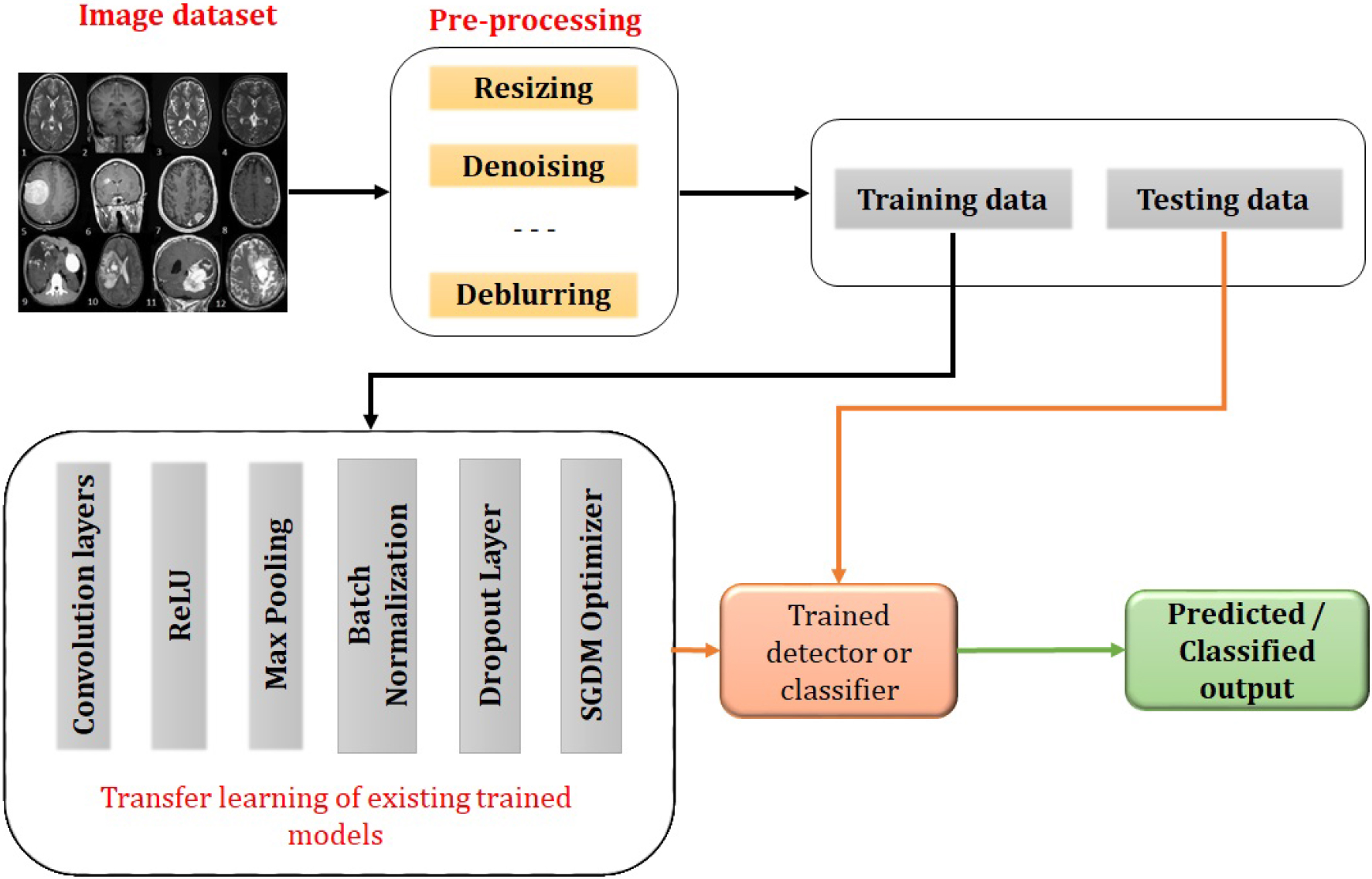

There are different modalities for healthcare radiological imaging like X-rays, Thermal imaging, Ultrasound imaging, Computer Tomography (CT) scanning, Positron Emission Tomography (PET) scanning, Magnetic Resonance Imaging (MRI), etc [22, 23, 24]. MRI is most suitable for soft tissues. Also, it can be used to measure the size of the tumor. But one sequence may not be sufficient for obtaining the entire information about the tumor. Different types of MRI are used for different applications. Intravenous (IV) gadolinium-enhanced MRI can capture the tumor very clearly, diffusion-weighted imaging can capture the structure of the brain, perfusion imaging show the quantity of blood flowing to the tumor, spinal MRI can capture the details of tumor near the spine, functional MRI (fMRI) gives the location of the tumor and Magnetic resonance spectroscopy (MRS) provides the information regarding the chemical composition of the brain. Generally, different MRI sequences like T1, T1c, T2, and T2FLAIR are employed for diagnosis purposes. T1 is the most commonly used sequence for analyzing the structure of the brain, but the border of the tumor area appears brighter in T1c. The edema region is brighter in T2 and T2FLAIR helps in the separation of the edema region from the cerebrospinal fluid (CSF).

A doctor can use Computer Aided Diagnostic (CAD) tools as a second opinion for analyzing brain tumors and thus these tools are developing rapidly in the last few decades. The CAD tools have major applications in both Macro and Micro Medical imaging [25, 26]. There are different CAD tools available for diagnosis purposes. These provide Graphical User Interfaces (GUI) which makes them more user-friendly. The requirement to design a CAD system is that the brain images acquired by the MRI scanners are to be read by the system in order to estimate the size, shape, and extent of the tumor and then it has to be classified into various classes.

In this paper, a detailed description of existing methods for brain tumor detection from brain MRI data is included. The main contribution of this paper is the detailed analysis of 19 different DL models for brain tumor detection and classification. Section 2 describes various brain tumor detection techniques followed by the proposed method in Section 3, the dataset in Section 4, the result and discussion in Section 5 and finally concluding in Section 6.

2. Brain Tumor Detection and classification

Brain Tumor Detection (BTD) means detecting whether a tumor is present in MRI data or not. Brain Tumor Classification (BTC) is for classifying the MRI tumor data into different classes. BTD and BTC can be treated as a single problem or as two different problems. BTD can be considered as a two-class classification problem with classes such as MR image with and without tumor. If more types of tumors are incorporated, then it becomes a pure classification problem.

In the 1970s, image processing techniques were used for the detection and classification of brain tumors. Image compression and feature transgeneration [27] can be used for designing computer-aided-diagnosis of brain tumors from scintigraphic images. KL transform was used for obtaining the optimal representation of the image data and the optimum Bayes rule was used for pattern recognition in order to identify whether the input image was normal or abnormal. The first edition of classification of the central nervous system (CNS) tumors was published in 1979 [31] by World Health Organization (WHO) followed by the second edition in 1993 [29, 30, 31, 32, 33, 34, 35], the third edition in 2000 [36] and the revised edition in 2007 [34]. According to the second edition, more than 150 types of CNS tumors are mainly classified as primary and secondary tumors [33].

An expert system based on an unsupervised clustering algorithm [35] can analyze the tissue area and provide a label for classifying it as normal or abnormal. A kNN classifier for BTC which gave the probabilistic information regarding the tissue model was proposed by Kaus et al. [28]. The possibility of variable selection [64] was investigated and kernel-based probabilistic classifiers like BayLSSVMs and RVMs were used as classifiers for two-class and multiclass classification. Carlos et al. [37] proposed a method for the classification of three-dimensional volume based on the occlusion of voxels collectively known as occlusion spectrum to form an occlusion transfer function. This was one of the first of this kind for 3D volumetric analysis. A fast unsupervised change detection method [38] was explored for detecting the boundary of the tumor.

Glioblastoma multiforme (GBM) in magnetic resonance can be detected and segmented using Support Vector Machine (SVM) and affinity metric models in [39]. Here, the models were trained using the features extracted from the superpixels by Gabor wavelet filters. An eight-class classifier based on sparse representation was validated using the Leave-two-out cross-validation technique in [40]. Syed et al. [41] used Multi-fractal Detrended Fluctuation Analysis (MFDFA) and multi-fractional Brownian motion for BTC. Another method based on SVM, Artificial Neural Network (ANN), temper-based K-means, and modified Fuzzy C-means (TKFCM) clustering algorithm was proposed by Ahmmed et al. [42]. Here, SVM was used for detecting tumor images and isolating normal images and ANN was used for classifying the tumor images into benign and four types of malignant tumors. Nilesh et al. [43] proposed Berkeley wavelet transformation (BWT) based BTS and SVM based BTC to improve the accuracy.

The features like intensity, differences in intensity, local neighborhood, and wavelet texture were integrated to train the random forest classifier for predicting five different classes in [44]. After classification, class labels were used for computing three different regions an active tumor, an enhancing tumor, and a complete tumor. Javeria et al. [45] suggested an automatic method using SVM classifier with different cross-validation based on features extracted from shape, texture, and intensity for classifying the cancerous and non-cancerous MR images. A hybrid approach by incorporating discrete wavelet transform (DWT), Genetic algorithm, and support vector machine (SVM) was presented in [46] for classifying brain tumors as benign or malignant. The different parameters used were smoothness, kurtosis, entropy, RMS, and correlation. The five-fold cross-validation was performed in [47] to improve the accuracy of validating a method based on CNN and a fully connected network.

Berkan et al. [48] proposed a BTD method based on a probabilistic neural network (PNN). At first, a clustering algorithm was applied and then thresholding and level-set segmentation were applied followed by PNN based classification. A lightweight Deep Neural Network was developed by Javeria et al. [49] and validated by using eight challenging brain tumor datasets. A DNN classifier combined with DWT and PCA was developed for classifying the input images into 4 different classes [50]. Another system using machine learning based back propagation neural networks (MLBPNN) was presented in [51] to enhance the exactness of BTC. The features were extracted using a fractal dimension algorithm, gray level co-variance matrix (GLCM), and principal component analysis (PCA). Sajjad et al. [52] suggested a Deep CNN based multi-grade BTC. At first, the tumor regions were segmented using Input Cascade CNN and then data augmentation was performed for training the modified VGG-19 architecture.

A clinical support system for BTC using Genetic Optimized Median Filter (GOMF) and Hierarchical Fuzzy Clustering Algorithm (HFCA) was proposed by Rupa et al. [53]. The feature extracted using GLCM was used for training the Lion Optimized Boosting SVM model. A classification method based on pre-trained models like Alexnet and VGGnet [54] for classifying benign and malignant tumor cases suggested that a pre-trained network can be effectively used for the classification of other objects. Other sets of pre-trained classifiers were proposed by Neelum et al. [55] using pre-trained models like Inception-v3 and DensNet201. The features extracted by both networks were concatenated to create the final model. A DL Network was trained as a discriminator in a GAN and then the fully connected layers were replaced and the final network was trained as a classifier for classifying into meningioma, glioma, and pituitary tumor in [56]. Jia et al. [57] suggested a Fully Automatic Heterogeneous Segmentation using Support Vector Machine (FAHS-SVM) based on structural and morphological details for BTS to separate the cerebral nervous system into MR images. The accuracy of the BTD system was verified by a probabilistic neural network classification system.

Table 1
Different BTD and BTC methods available in the literature

Literature	Year	Methodology	Dataset	Result
Han et al. [25]	1973	Image compression and feature transgeneration	Brain scan data	Accuracy 80 to 89%
Chunlin et al. [35]	1993	Unsupervised clustering algorithm		Accuracy – 88.89%
Kaus et al. [28]	2001	kNN classifier	Data generated from MRI system	Accuracy – 95%
Chuan et al. [36]	2007	Bayesian learning, BayLSSVMs and RVMs	Microarray dataset	2-class accuracy – 96 to 99.7% and
				Multiclass accuracy – 84 to 89.95%
Carlos et al. [37]	2009	Occlusion spectrum	CT volumetric dataset	Images with unprecedented clarity and
				quality
Saha et al. [38]	2011	Unsupervised change detection and Bhattacharya coefficient	MRI dataset	Dice – 52 to 57%
Wei et al. [39]	2013	Gabor wavelet filters, SVM and affinity metric model	MICCAI 2012	Jaccard – 60 to 91%
Muhammad et al. [40]	2014	Sparse representation and Leave-two-out cross-validation technique	–	Accuracy – 97.5%
Syed et al. [41]	2015	MFDFA and multifractional Brownian motion	BRATS	Accuracy – 83%
Ahmmed et al. [42]	2017	SVM, ANN, k-means and fuzzy c-means clustering algorithms	Clinical data	Accuracy – 97.37%
Nilesh et al. [43]	2017	BWT and SVM	DICOM and Brain Web dataset	Accuracy – 96.51%
Khalid et al. [44]	2017	Random Forest	BRATS 2013	Dice – 75 to 95%
Javeria et al.[45]	2017	SVM	Harvard, RIDER and Local	Accuracy – 97.1%
Sanjeev et al. [46]	2017	DWT, Genetic Algorithm and SVM	SICAS Medical Image Repository	Accuracy – 80 to 91.2%
Justin et al. [47]	2017	CNN and fully connected networks	public brain tumor dataset	Accuracy – 91.43%
Berkan et al. [48]	2017	PNN	BRATS 2016	Accuracy – 85 to 90%
Javeria et al. [49]	2018	DNN	BRATS 2012-15 and ISLES 2015-17	Accuracy – 93.1 to 100%
Heba et al. [50]	2018	DNN with DWT and PCA	Harvard	Accuracy – 93.9 to 98.4%
Shakeel et al. [51]	2019	MLBPNN, GLCM and PC	SPL	Accuracy – 95.1%
Sajjad et al. [52]	2019	VGG-19	Radiopaedia and Brain tumor dataset	Accuracy – 90.67 & 94.58%
Rupa et al. [53]	2019	GOMF, HFCA and SVM	BRATS	Accuracy – 97.69%
Amin et al. [54]	2019	Alexnet & Googlenet	BRATS 2013-16 & ISLES 2018	Accuracy – 72.27 to 99.71%
Neelum et al. [55]	2020	Inception-v3 & DensNet201	3 class brain tumor dataset	Accuracy – 99.51%
Navid et al. [56]	2020	GAN	Public brain tumor dataset	Accuracy – 93.01 to 95.6%
Jia et al. [57]	2020	FAHS-SVM	Multi-spectral brain dataset	Dice – 85 to 97%
Pei et al. [58]	2020	3D-CNN	BRATS 2019	Dice – 63.9%
Jeevanantham et al. [59]	2020	Gabor transform, EML and CANFIS	BRATS 2016	99.3%
Kumar et al. [60]	2021	RNGAP	Public brain tumor dataset	Accuracy – 97%
Deepak et al. [61]	2021	CNN & SVM	Figshare	Accuracy – 95.82%
Sharif et al. [62]	2021	EKbHFV, MGA and SVM	BRATS 2018 & 2019	Accuracy – 95%
Kokkalla et al. [63]	2021	Inception-ResNet-v2	public brain tumor dataset	Accuracy – 99.69%
Bala et al. [64]	2021	CNN	Public brain tumor dataset	Accuracy – 97.52%
Pallavi et al. [65]	2021	Hanman-Shannon transform	BRATS 2018	Accuracy – 99%
Abdul et al. [66]	2022	CNN	Kaggle	Precision – 92.13%
Ayesha et al. [68]	2022	Ensemble model	Brain MRI Images	Accuracy – 98.14%
Lakshmi et al. [69]	2022	Inception-V3	Figshare	Accuracy – 89%
Jun et al. [70]	2022	Multipath CNN	Figshare	Accuracy – 98.61%

Pei et al. [58] applied a three-dimensional Convolutional Neural Network (3D-CNN) on the tumor segments segmented using 3D context-aware deep learning for tumor classification and performed a hybrid method of DL and ML for survival prediction. This has received second place in the 2019 CPM-RadPath global challenge. Jeevanantham et al. [59] used Gabor transform for converting the denoised images into multi-orientation based brain images. The hybrid features were extracted and classified the images were into normal and abnormal using the extreme machine learning (EML) method. Finally, the segmented regions were diagnosed using an adaptive neuro-fuzzy inference system (CANFIS) classifier to classify them into severe or mild. Another transfer learning approach based on ResNet-50 and the global average pooling (RNGAP) model was developed as a solution to vanishing gradient and over-fitting problems in [60].

A fully automated medical image classification technique as a combination of CNN and SVM was proposed by Deepak et al. [61]. Another transfer learning based approach used the pre-trained deep learning model Densenet201 model for classification purpose in [62]. The Entropy-Kurtosis-based High Feature Values (EKbHFV) and modified genetic algorithm (MGA) were used for feature selection and these features were fused to train the multiclass SVM cubic classifier. Kokkalla et al. [63] suggested a three-class BTC framework based on a deep dense inception residual network by customizing the output layer of Inception-ResNet-v2 architecture with a deep dense network. Bala et al. [64] proposed a seven-layer CNN for multi-class brain magnetic resonance (MR) image classification into three different classes. A classification method based on higher level probabilistic uncertainty for developing the possibilistic Hanman-Shannon transform classifier was proposed by Pallavi et al. [65].

A classification model for classifying brain tumor data into four classes – glioma, meningioma, pituitary tumor, and no-tumor using the CNN model was proposed by Abdul et al. [66] and they got a precision of 92.13%. Arabahmadi et al. [67] presented a comparative analysis of different techniques used for BTD, different types of available datasets, and the research directions in this area. Ayesha et al. [68] developed an ensemble model using a combination of deep learning and transfer learning based on VGG-16 and LSTM networks for obtaining a remarkable accuracy rate. Brain tumor classification based on Inception-V3 with adam optimizer was proposed by Lakshmi et al. [69] and they got an accuracy of 89%. Jun et al. [70] proposed another CNN approach for BTD using a guided multipath network and obtained an accuracy of 98.61%. Solanki et al. [71] proposed several ways to detect brain tumors and cancer. It also explained brain tumor morphology, different datasets, augmentation techniques, and transfer learning based approaches. The details of all the above discussed methods for BTD and BTC are consolidated in Table 1 along with the information regarding the dataset and the final output.

3. Transfer learning based proposed system

Transfer learning is a method of retraining the pre-trained deep learning models for making them suitable for a particular detection or classification application. There are so many efficient classification models available in the literature like AlexNet, VGGnet, SqueezeNet, ShuffleNet, GoogleNet, ResNet, Inception, Xception, DenseNet, DarkNet, NasNet and their various versions as discussed earlier. These models can be utilized for BTD and BTC via the method of deep transfer learning. We can transfer the learning gained by the pre-trained model starting from the very first layer till the last layer or some selected layers towards the end of the model.

In this paper, we have adopted the second method where we have replaced the last three layers of each of the networks to create two class classifiers and four class classifiers. We have selected 19 different pre-trained classification models given in Table 2 which are capable of classifying 1000 classes according to the ImageNet Challenge [72]. The Table is organized in the increasing order of performance in terms of classification accuracy. AlexNet [73] is basically a CNN that is capable of classifying objects into 100 classes. This is the pre-trained network with less complexity when compared to other models in terms of the number of layers. GoogleNet [74] is the advanced form of LeNet, an efficient 10-class classifier. This has an “inception module” which performs convolution using different sizes of filters and finally concatenates the outputs to form the input of the next layer.

Table 2
Different characteristics of the pre-trained network models

Sl No:	CNN architecture	Filter(s) size	Input size	No. of convolutional layers	No. of parameters (millions)
1	AlexNet	11x11, 5x5, 3x3	227x227x3	8	62.57
2	SqueezeNet	3x3, 1x1	224x224x3	18	1.2
3	ShuffleNet	3x3, 1x1	224x224x3	50	1.4
4	GoogleNet	3x3	224x224x3	22	4
5	ResNet-18	3x3	224x224x3	18	11.7
6	MobileNet-V2	3x3, 1x1	224x224x3	28	3.4
7	VGG-16	3x3	224x224x3	16	4
8	VGG-19	3x3	224x224x3	19	139
9	NASNet Mobile	1x1, 1x7, 7x1, 3x3, 5x5, 7x7	224x224x3	–	5.3
10	DarkNet-19	3x3	256x256x3	19	20.8
11	ResNet-50	3x3, 1x1	224x224x3	50	25.6
12	DenseNet-201	3x3, 1x1	224x224x3	201	20
13	ResNet-101	3x3, 1x1	224x224x3	101	44.6
14	DarkNet-53	3x3, 1x1	256x256x3	53	41.6
15	ResNet-152	3x3, 1x1	224x224x3	152	58.5
16	Inception-V3	5x5, 3x3, 1x1	299x299x3	48	23.9
17	Xception	3x3	299x299x3	71	22.9
18	Inception-ResNet-V3	1x1, 3x3, 5x5	299x299x3	164	55.9
19	NASNet Large	1x1, 1x7, 7x1, 3x3, 5x5, 7x7	331x331x3	–	88.9

In VGGnet [75], VGG stands for Visual Geometry Group and it has two variants VGG16 and VGG19. From the name itself, we can understand that they differ in the number of layers as shown in Table 2. It is more complex with 138 million parameters, but it is an efficient feature extractor for many applications. The ShuffleNet is another efficient classifier that uses point-wise group convolution known as “1x1 convolution” and channel shuffling to reduce computational complexity while maintaining accuracy. They have introduced the ShuffleNet [76] units in three stages for varying the number of channels. SqueezeNet [77] consists of a “fire module” comprising of a squeeze convolution layer having 1x1 convolutional filters and an expand layer having both 1x1 and 3x3 convolutional filters. These modules are reducing the parameter space to a great extent. Different versions like Vanilla SqueezeNet, SqueezeNet with simple bypass, double bypass, etc. are there. Here, we have adopted vanilla SqueezeNet.

MobileNet [78] is a CNN that uses depth-wise separable convolutions. It reduces the parameter space and is lightweight. The depth-wise separable convolution incorporates depth-wise convolution and point-wise convolution. DarkNet also has 2 variants – DarkNet-19 [79] and DarkNet-53 [80]. DarkNet-19 is the backbone of YOLO-v2 and DarkNet-53 is that of YOLO-v3. ResNet [81] has residual connections known as “skip connections” for decreasing the complexity of having more layers. It has multiple variants according to the number of layers. We have selected 4 among them namely ResNet-18, ResNet-50, ResNet-101, and ResNet-152. GoogLeNet has an Inception Module, which performs convolution operations using filters of different sizes and concatenates the outputs for the next layer. AlexNet, on the other hand, has layer input provided by one previous layer instead of a filter concatenation.

The inception network [82] is the modified version of GoogleNet that incorporates more “inception module” which contains a concatenation layer to make it learn more deeply and faster than GoogleNet. The number of channels gets reduced due to the presence of 1x1 convolution which is responsible for feature space compression followed by 3x3 and 5x5 filters which are capable of learning patterns across the depth of the input image. The representational power is also less due to the varying filter size. There are different versions like Inception-v1, Inception-v2, Inception-v3 [83], Inception-v4 and Inception-ResNet. Among these, we have adopted Inception-v3 and Inception-ResNet-v3 [84]. Xception [85] stands for “Extreme Inception”. This also takes the same inception module concept but in reverse fashion. It applies other filters first on the depth map followed by 1x1 convolution for compression. Inception network introduces non-linearity while Xception doesn’t.

Neural Architecture Search Network (NASNet) [86] automates the development of neural network architectures. This algorithm can search for the best algorithm to achieve the most efficient performance on a certain task. The general setup involves Search Space, Search Strategy, and Performance Estimation Strategy. The basic idea was to search for the best combination of parameters from the given filter size, number of output channels, number of layers, strides, etc. NASNet is based on reinforcement learning. A new regularization technique called “ScheduledDropPath” was introduced that significantly improves the generalization of the NASNet models. This network consists of two types of cells – normal cells and reduction cells. Different types of filters are there for extracting the features at different levels. These features learned by NASNet can be incorporated with other networks for making it applicable to different types of classification problems. There are three major variants namely NASNet-A, NASNet-B and NASNet-C.

Figure 3.

Process flow of the proposed detectors.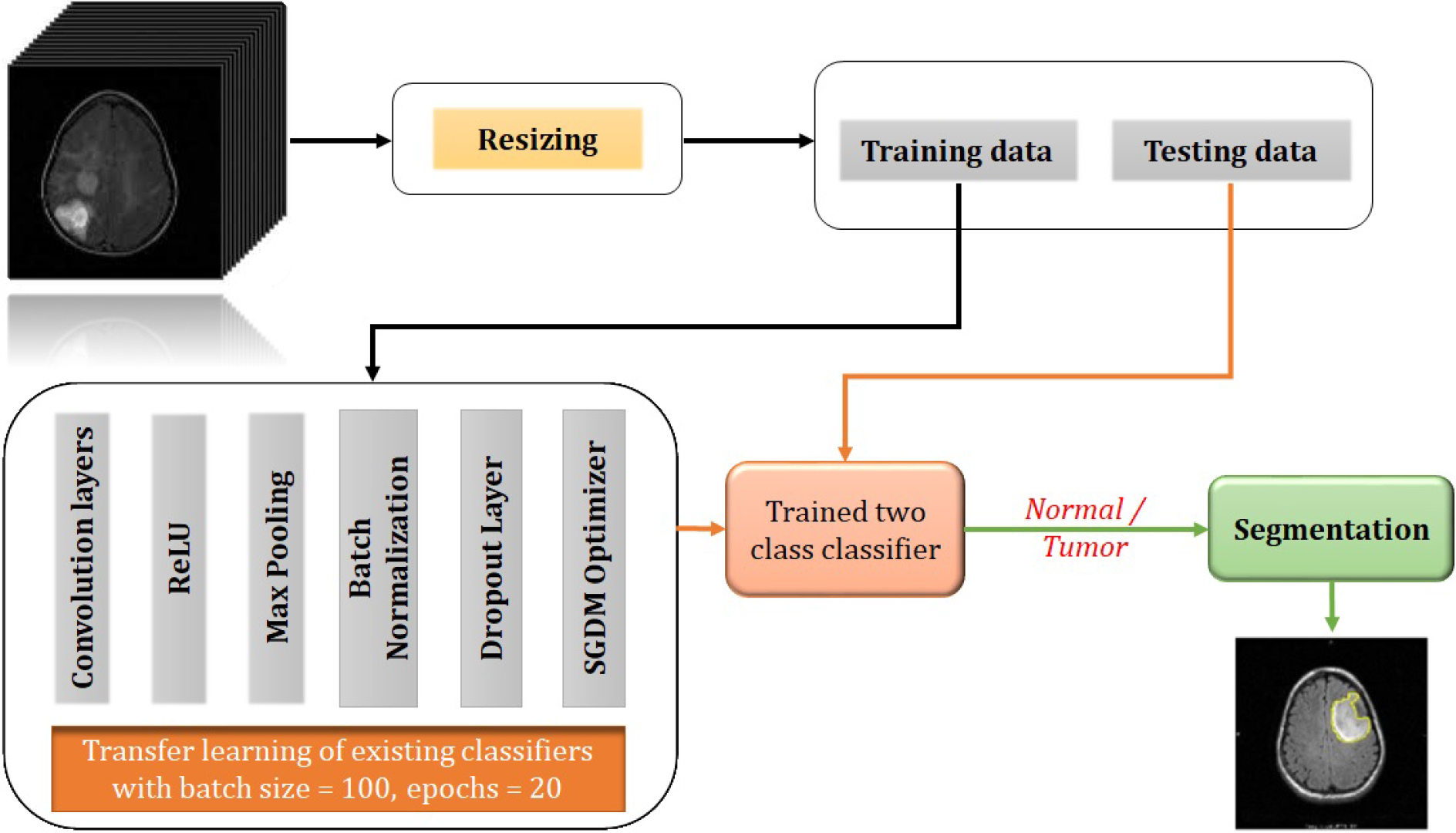

Figure 4.

Process flow of the proposed classifiers.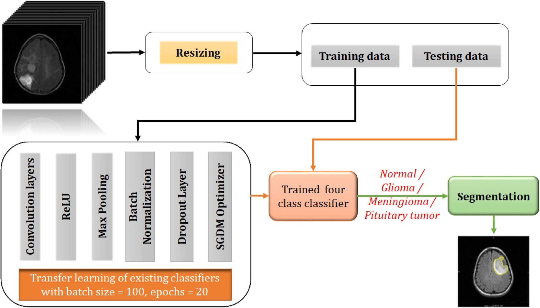

The process flow of the proposed detectors and classifiers are shown in Figs 3 and 4 respectively. At first, we are training the networks with the training dataset collected from the repository. We require an enormous amount of data to make the network learn properly as it is extracting the features on its own and reaching a good conclusion. If we can provide an approximately equal number of data samples of each class for training, the biasing problem can be exempted up to a limit. This might not be possible for all cases of classification problems. If we are not getting enough amount of data samples in each of the classes, we can make use of data augmentation techniques like SMOTE [87], ADASYN [88], etc. to balance the number of samples among classes. But these techniques may not be good for medical data augmentation as accuracy and precision are having the utmost importance in the medical field. Also, these can be applied if the percentage difference between the number of samples between classes is very high. The region characteristics should also be preserved as we are dealing with human tissue structures. Affine transformations [89] like rotation, translation, a combination of both, etc. can be used for data augmentation as they preserve the region characteristics. This can be considered as one type of pre-processing technique. Principal Component Analysis can also be used for data augmentation as in [90].

We need to provide the network with data having the same size as that of the size of the input layer of the network as we are using transfer learning approaches. Otherwise, the network might not work properly. So second type of pre-processing is resizing the input data according to the size of the input layer of the classifier. This pre-processed data is then divided into a training dataset and a testing dataset and the training dataset is given to the deep learning network for training. All the above networks are retrained via transfer learning of the last 3 layers for making them classify the input into tumor or normal in the case of detectors and four classes like Glioma, Meningioma, and Pituitary tumor in the case of classifiers. The last fully connected layer is replaced with a new one capable of producing the corresponding outputs. Also, the last layer is replaced with a 2-class classification layer in the case of detectors and a 4-class classification layer in the case of 4-class classifiers. The networks are then retrained for detection and classification purposes respectively. Another sort of retraining can also be done using different optimization algorithms as shown in [91]. If we are incorporating those methods here, we can optimize the network performance in terms of optimization algorithms too.

Here, we are presenting detection via the method of classification. The detectors are designed as 2-class classifiers for classifying into tumor or normal. From the output, we can conclude whether the tumor is present in the input image or not. We have labeled the tumor class as the positive class and the normal class as the negative class. After training, the trained network is tested using the testing dataset. If a testing query is given to the network, the network will test whether it is a normal image or a tumor image. If it is a normal image, then it will print only the input image. Otherwise, it will print the input image along with the segmented output as shown in Fig. 3. A simple thresholding algorithm based on solidicity and depth is used here for segmenting out the tumor area. The classifiers are trained for classifying into four classes – Normal, Glioma, Meningioma, and Pituitary tumor. If a testing query is given to the trained network, the network will test to find out to which class it belongs. If the classified output is a normal one, the segmentation part won’t work. Otherwise, the segmentation algorithm will work and the segmented output along with the input gets printed as the final output as shown in Fig. 4.

4. Dataset

Different datasets are available for brain tumor detection, classification, and segmentation. The Harvard Whole Brain Atlas dataset [92] consists of images in different modalities like CT, MRI, SPECT, etc. The second one is the Multimodal Brain Tumor Image Segmentation (BRATS) dataset [93]. Twenty different state-of-the-art brain tumor segmentation algorithms were incorporated into data consisting of 65 multi-contrast MR scans of different grades of glioma manually annotated by using tumor image simulation software. This was a result of the conferences MICCAI 2012 and 2013. After the challenge, this data is made publicly available for segmentation, detection, and classification. The Internet Brain Segmentation Repository (IBSR) [94] gives the manually segmented MR brain image data for BTS.

MRBrainS [95] is a dataset containing 3T MR images. This is an online evaluation framework for evaluating automatic and semi-automatic BTS algorithms. ILSVRC [96] is a challenge that started in 2010. This is running annually from 2010 to the present. This dataset is a huge collection of different objects and therefore this can be used for object recognition as well as classification. Another dataset available is the Cancer Imaging Archive (TCIA) [97]. It is an “open-source, open-access information resource to support research, development, and educational initiatives utilizing advanced medical imaging of cancer”. The Cancer Genome Atlas Project (TCGA) [98] is a publicly funded project initiated by National Cancer Institute to collect cancer data, both raw and processed and to make these data available to all researchers. The figshare dataset [99] contains 3064 T1-weighted contrast-enhanced images consisting of three different types of brain tumors. The information regarding the available datasets in the literature is consolidated in Table 3.

Table 3
Different datasets available in the literature

Dataset	Year	Purpose	Types
Harvard	2003	Classification	Different classes
BRATS	2013 to 2021	BTS	Meningioma, Glioma, Pituitary tumor, Glioblastoma (GBM/HGG) and low
			grade glioma (LGG)
IBRS	2007	BTS	3T Brain MRI scans
MRBrainS	2015	BTS	3T MR images
ILSVRC	2015	Classification	Different classes
TCIA	2013	Classification	Different classes
TCGA	2015	Classification	Different classes
Figshare	2017	Classification	Different classes

MRI data for BTD available in Kaggle is used for training and testing the developed networks. A total of 11722 MR images are there, among that 3250 are normal images and 8472 are images with tumors. As the number of normal images is less when compared to tumor images, we have applied affine transformations like rotation and translation for balancing the normal class. Rotation is changing the angular orientation of an image in a specific direction according to the angle specified in the rotation matrix and translation is changing the spatial orientation according to the amount of translation in the x and/or y direction. If there is a reference point that can be taken as the origin, we can reduce affine transformation to a linear transformation. For example, if we can describe a transformation as a rotation by a fixed angle with respect to an axis, then it can be defined as a combination of rotation and translation processes. We can apply any of these operations or both for getting the augmented images as shown in Fig. 5. The obtained augmented dataset consists of 6500 normal images. The tumor class contains more than double the number of images when compared to the normal class. So, we intended to make the number of normal images as twice that contained in the original dataset to make it almost comparable with the number of images in the tumor class. Thus, we applied only affine transformations to create the augmented data. From the full dataset containing the original data and the augmented data, 80% images from each class are used for training, and 20% are used for testing. We have tried with 70-30, 80-20, and 90-10 proportions. But 80-20 proportion gave promising results. Further details of the dataset are given in Table 4.

The figshare dataset is used for classification purposes. This dataset consists of 3064 MR images corresponding to three classes of brain tumors – glioma, meningioma, and pituitary tumor. Among these 1426 belong to the class glioma, 708 belong to the class meningioma and 930 belong to the class pituitary tumor. We have incorporated the 3250 normal images from the Kaggle dataset along with this dataset for making the dataset consist of 4 classes – normal, glioma, meningioma, and pituitary tumor. Here also we have applied affine transformation like rotation and/or translation for balancing the number of samples in all the classes and finally, we got the number of samples as shown in Table 5. Among these, 80% are used for training purposes and the remaining 20% for testing purposes.

Table 4

Dataset used for the detector networks

	Normal	Tumor	Total
Actual dataset	3250	8472	11722
Augmented dataset	6500	8472	14972
Training dataset (80%)	5200	6778	11978
Testing dataset (20%)	1300	1694	2994

Table 5

Dataset used for the classifier networks

	Normal	Glioma	Meningioma	Pituitary tumor	Total
Actual dataset	3250	1426	708	930	6314
Augmented dataset	3250	2852	2832	2790	11724
Training dataset (80%)	2600	2282	2266	2232	9380
Testing dataset (20%)	650	570	566	558	2344

Figure 5.

Affine transformation (a) Input tumor image of size 512x512x3, (b) Rotation by an angle 45 degree, (c) Translation by (50,50) and (d) Rotation by 45 degree followed by translation by (125,125).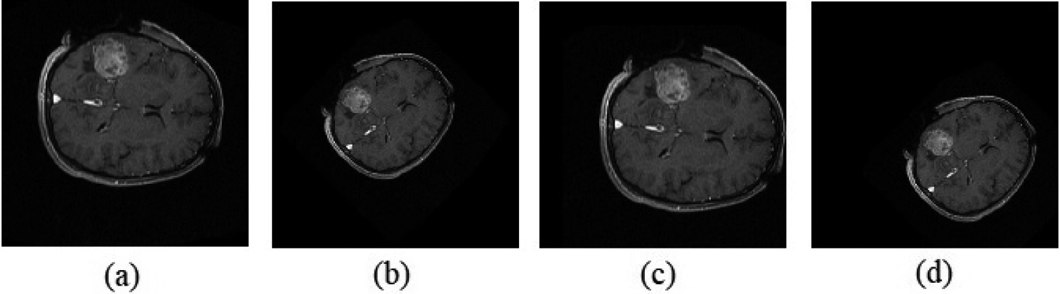

Figure 6.

Confusion matrices of 2-class classifiers (detectors) using (a) Xception, (b) Inception-ResNet-V3 and (c) NASNet Large.

5. Results and discussion

Deep transfer learning based approaches [100] to retrain 19 different deep learning networks for brain tumor detection and classification purposes are presented here. Thus we have presented 19 different detectors and 19 different classifiers using well-trained models like AlexNet, GoogleNet, VGGNet, SqueezeNet, ShuffleNet, MobileNet, ResNet, DarkNet, InceptionNet, NASNet, and their variants. The stochastic gradient descent optimization algorithm is used for retraining with a batch size of 100 and epochs of 20. For all networks, the last 3 layers are modified for making them suitable for brain tumor detection and classification. The training and validation accuracies and loss curves of Xception, Inception-ResNet-V3, and NASNet Large during the training process are shown in Fig. 6a–c respectively. The graph represented in blue color is showing the training accuracy versus iterations and that represented in red color is showing the loss versus iterations. From these Figures, it is evident that the network is properly trained as the training accuracy is increasing from lowest to almost 100% and the loss is decreasing from maximum to zero at the final iteration. The validation accuracies obtained for Xception, Inception-ResNet-V3, and NASNet Large are 98.12%, 98.93%, and 99.26% respectively. These curves infer that among the trained networks NASNet Large is outperforming all the other models.

Figure 7.

Output of the detector corresponding to the class “Tumor”. (a) Tumor image, (b) Segmented area and (c) Tumor region shown in the input image.

Figure 8.

Output of the detector corresponding to False Positive. (a) Normal image, (b) Segmentation output and (c) Normal region falsely identified as tumor.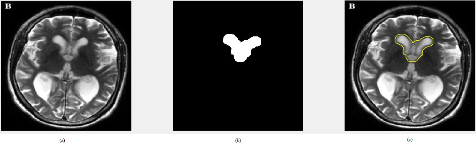

Figure 9.

Output of the detector corresponding to False Negative. (a) Tumor image, (b) Segmentation output and (c) Tumor region is not identified.

Figure 10.

Output of the classifier corresponding to the class “Glioma”. (a) Glioma image, (b) Segmented area and (c) Tumor region shown in the input image.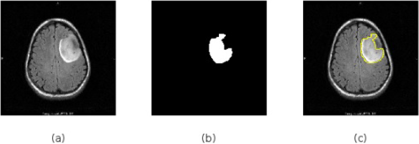

Figure 11.

Output of the detector corresponding to the class “Meningioma”. (a) Meningioma image, (b) Segmented area and (c) Tumor region shown in the input image.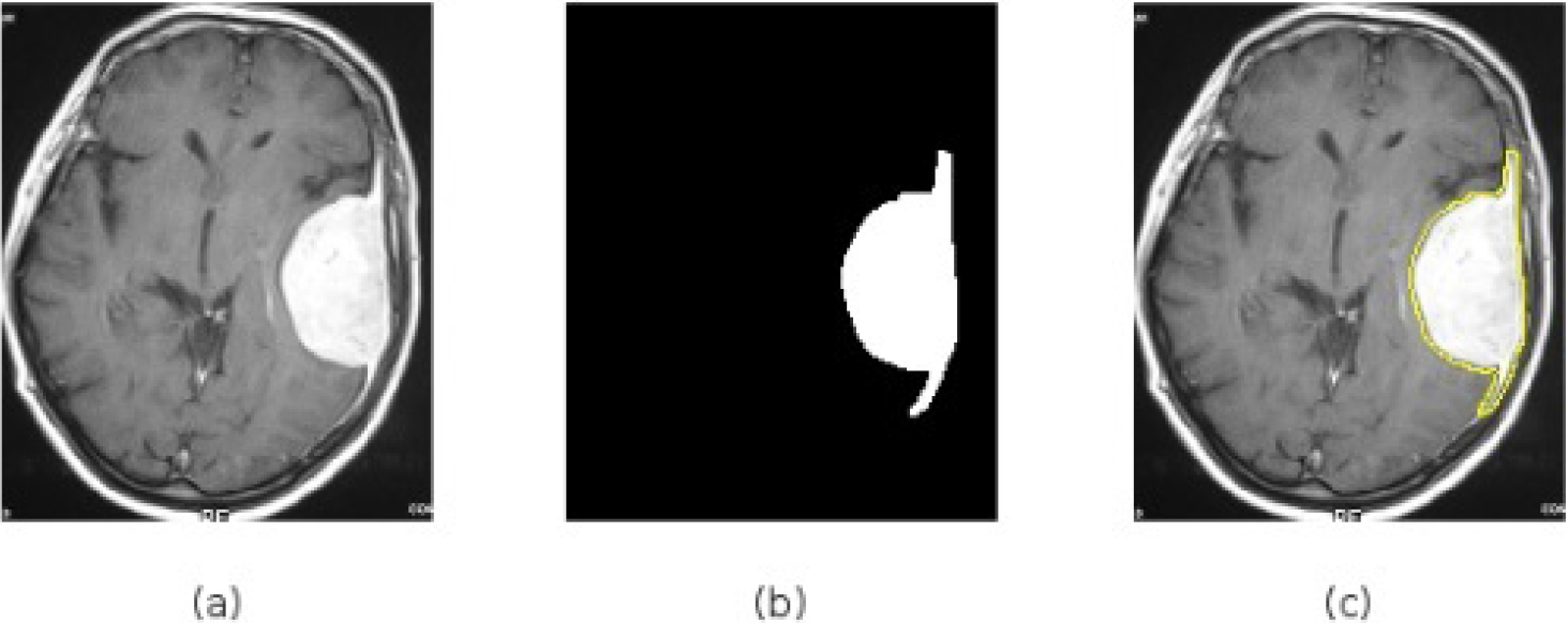

Figure 12.

Output of the detector corresponding to the class “Pituitary tumor”. (a) Pituitary tumor image, (b) Segmented area and (c) Tumor region shown in the input image.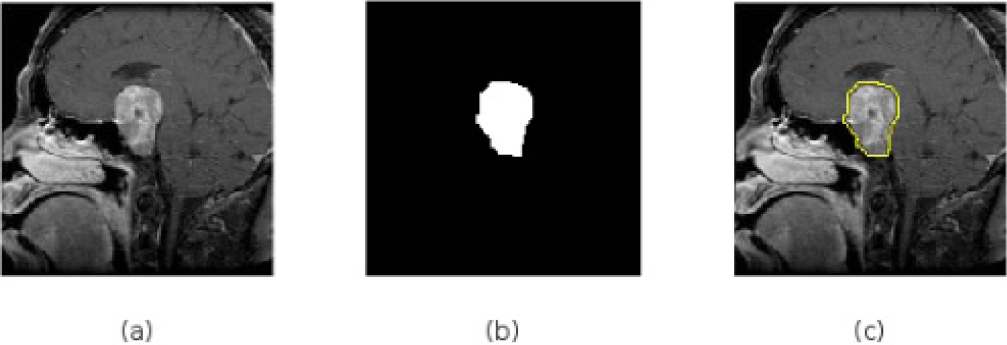

Figure 13.

Confusion matrices of 2-class classifiers (detectors) using (a) Xception, (b) Inception-ResNet-V3 and (c) NASNet Large.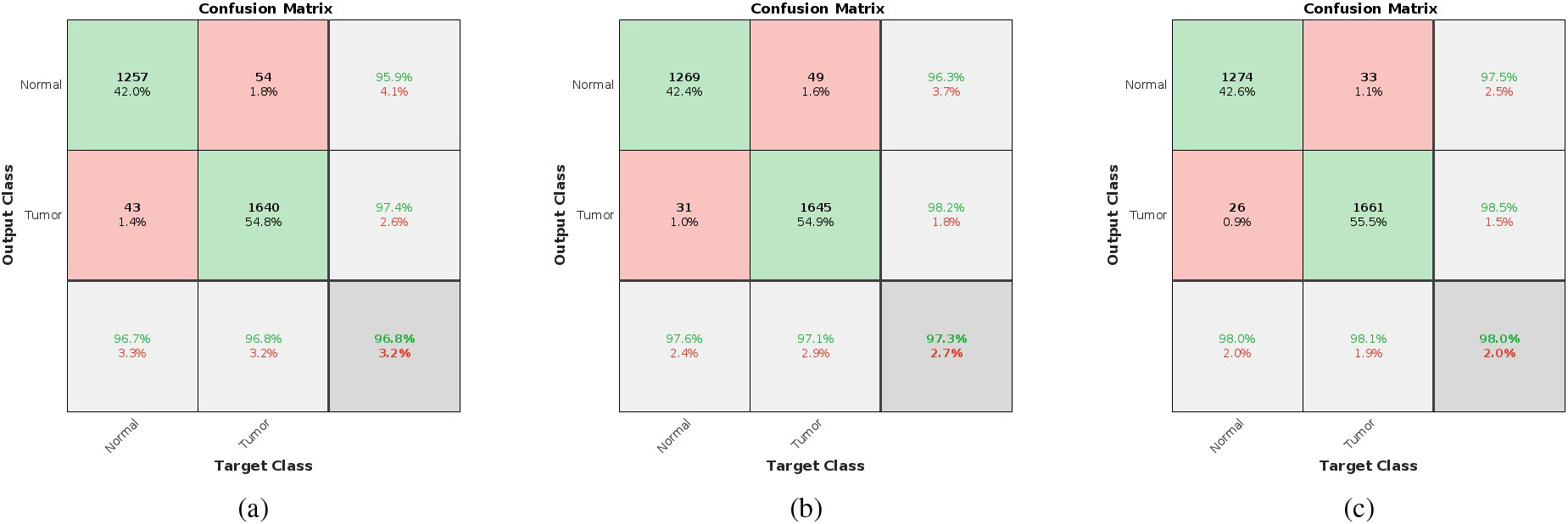

Figure 14.

Confusion matrices of (a) Xception, (b) Inception-ResNet-V3 and (c) NASNet Large.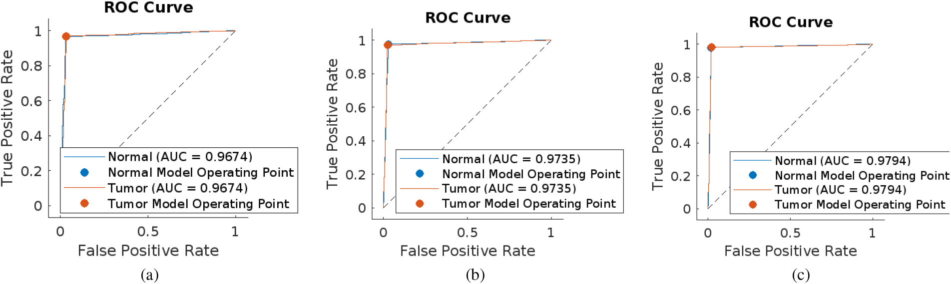

Figure 15.

Confusion matrices of 2-class classifiers (detectors) using (a) Xception, (b) Inception-ResNet-V3 and (c) NASNet Large.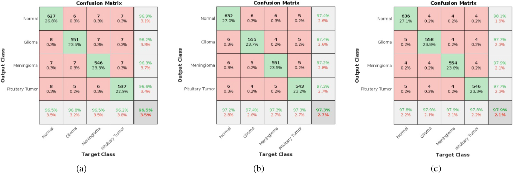

Figure 7 shows the output corresponding to the detectors if the detected output is in class “Tumor”. It shows the input MR image, the tumor area segmented out and the MR image with the tumor area projected with boundary. Figure 8 shows the case of a false positive in which the normal region in an input image is identified as a tumor region and hence the input image is detected as in tumor class. Figure 8a represents the normal image, whereas 8b and 8c represent the segmented image and false positive output respectively. Figure 9 shows the case of a false negative where the detector missed the tumor region and detected the image as a normal image. Figure 9a represents the tumor image, whereas 9b and 9c represent the segmented image and false negative output respectively. Through the obtained output we can understand that the tumor is not identified by the detector. Figures 10–12 are showing the outputs of the classifiers for various classes. Figure 10 shows the output corresponding to the class “Glioma”, Fig. 11 that of “Meningioma” and Fig. 12 that of “Pituitary tumor”. For all these Figures, the first image is the input image followed by the segmented version of the affected region and the third one corresponds to the tumor area projected in the input image.

The confusion matrices [101] obtained for the most efficient brain tumor detection networks like Xception, Inception-ResNet-V3, and NASNet Large are shown in Fig. 13. Here, green color grids correspond to the true cases and pink color grids correspond to the false cases. We have considered the normal class as a negative class and the tumor class as a positive class. For example, Fig. 13c shows the confusion matrix of the NASNet Large detector. A total of 1300 normal images and 1694 tumor images are given for testing according to Table 5. Out of the 1300 normal images, 1274 are detected as normal (true negative) and the remaining 26 are detected as tumors (false positive). Similarly, 1661 out of 1694 tumor images are detected as tumors (true positive) and the remaining 33 are detected as normal (false negative).

The corresponding Receiver Operating Characteristics (ROCs) of all the above 3 detectors are shown in Fig. 14. In each of the ROC curves, the blue line indicates the variation of the true positive rate with respect to the false positive rate of the Normal class, and the red line that of the Tumor class. Alexnet is having the least area-under-the-curve (AUC) value and NASNet Large has the most. The performance parameters like true positive (TP), true negative (TN), Precision, Recall, F1 score, AUC, accuracy, and testing time of all the detectors corresponding to a single image are shown in Table 6. The accuracy of the networks is increasing from 83.17% provided by Alexnet to 98.03% provided by NASNet Large. Precision and recall values are also increasing manner. From Table 7, it is evident that NASNet Large is providing the maximum accuracy. Also from the obtained AUC values and F1 scores, we can conclude that the accuracies obtained are correct without any biasing or overfitting problems. Even though there is a huge difference in the number of parameters of the best three models Xception, Inception-ResNet-V3, and NASNet Large as in Table 2, their accuracies do not differ much. From Table 6, the accuracies of these models for detection are respectively 96.76%, 97.33%, and 98.03%. Also, the testing times for identifying the presence of tumor in an MR image for these models are 12.57 secs, 15.2 secs, and 19.18 secs respectively. Table 7 shows that the accuracies of these models for classification are respectively 96.46%, 97.31%, and 97.87%. Also, the testing times for classification are 13.47 secs, 15.57 secs, and 19.54 secs respectively. These accuracy values and testing times show that the performance of these models is really comparable even though the number of parameters are differing so much. As far as these values are concerned, we can ignore the difference in the number of parameters as in the medical field accuracy is having utmost importance.

Table 6

Performance parameters of various detection networks

Sl No:	CNN architecture	TN (out of 1300)	TP (out of 1694)	Overall true cases (out of 2994)	Precision (%)	Recall (%)	F1 score	AUC	Accuracy (%)	Testing time (secs)
1	AlexNet	1080	1410	2490	86.5	83.2	84.81	0.8333	83.17	1.2
2	SqueezeNet	1100	1433	2533	87.8	84.6	86.17	0.8446	84.6	1.05
3	ShuffleNet	1106	1444	2550	88.2	85.2	86.67	0.8535	85.17	1.4
4	GoogleNet	1119	1459	2578	89.0	86.1	87.52	0.8612	86.11	1.57
5	ResNet-18	1125	1467	2592	89.3	86.6	87.93	0.8627	86.57	1.5
6	MobileNet-V2	1133	1477	2610	89.8	89.2	89.5	0.8732	87.17	3.02
7	VGG-16	1145	1493	2638	90.6	88.1	89.33	0.8849	88.11	7
8	VGG-19	1158	1510	2668	91.4	89.1	90.24	0.8906	89.11	10.05
9	NASNet Mobile	1167	1521	2688	92.0	89.8	90.89	0.8988	89.78	4.03
10	DarkNet-19	1180	1538	2718	92.8	90.8	91.79	0.9097	90.78	6.07
11	ResNet-50	1185	1545	2730	93.1	91.2	92.14	0.9116	91.18	2.51
12	DenseNet-201	1204	1570	2774	94.2	92.7	93.44	0.9271	92.65	16.37
13	ResNet-101	1212	1582	2794	94.7	93.4	94.05	0.9313	93.32	4.55
14	DarkNet-53	1228	1603	2831	95.7	94.8	95.25	0.9464	94.56	11.1
15	ResNet-152	1230	1605	2835	95.8	94.7	95.25	0.9478	94.69	11.45
16	Inception-V3	1243	1622	2865	96.6	95.7	96.15	0.9558	95.69	8.12
17	Xception	1257	1640	2897	97.4	96.8	97.1	0.9674	96.76	12.57
18	Inception-ResNet-V3	1269	1645	2914	98.2	97.1	97.65	0.9735	97.33	15.2
19	NASNet Large	1274	1661	2935	98.5	98.1	98.3	0.9794	98.03	19.18

Table 7

Performance parameters of various classification networks

Sl No:	CNN architectures	Normal	Glioma	Meningioma	Pituitary tumor	Accuracy	Testing time (sec)
1	AlexNet	539	475	467	460	82.81	1.32
2	SqueezeNet	543	479	471	465	83.53	1.13
3	ShuffleNet	549	483	477	471	84.47	1.45
4	GoogleNet	558	490	485	475	85.67	2.05
5	ResNet-18	562	494	489	482	86.48	1.55
6	MobileNet-V2	566	499	492	485	87.12	3.55
7	VGG-16	571	502	496	489	87.80	7.31
8	VGG-19	578	508	502	493	88.78	10.35
9	NASNet Mobile	583	512	507	500	89.68	4.23
10	DarkNet-19	589	519	512	503	90.57	6.45
11	ResNet-50	592	524	516	509	91.34	3.01
12	DenseNet-201	601	530	523	515	92.53	17.39
13	ResNet-101	605	534	526	519	93.17	5.03
14	DarkNet-53	613	540	530	522	94.07	11.55
15	ResNet-152	614	542	530	523	94.24	12
16	Inception-V3	620	546	539	532	95.44	8.52
17	Xception	627	551	546	537	96.46	13.47
18	Inception-ResNet-V3	632	555	551	543	97.31	15.57
19	NASNet Large	636	558	554	546	97.87	19.54

The confusion matrices of 4-class classifiers are shown in Fig. 15. The diagonal elements are showing the true cases in the order normal, glioma, meningioma, and pituitary tumor and finally the classification accuracy. For example, in Fig. 14c 636 out of 650 Normal images, 558 out of 570 Glioma images, 554 out of 566 Meningioma images, and 546 out of 558 Pituitary tumor images are correctly classified with individual class accuracies of 97.8%, 97.9%, 97.9%, and 97.8% respectively and an overall network accuracy of 97.87%. The performance parameters of all the 4-class classifiers consolidated from the confusion matrices are shown in Table 7 along with the testing time of a single image. The Table is organized in terms of increase in accuracy. From this Table, it is evident that NASNet-Large is the most efficient among the 19 classifiers by providing an accuracy of 97.87%, but the testing time is maximum. Here also, that may not be a big problem as in the medical field accuracy is having utmost importance. All the 38 networks discussed so far are implemented in the Deep Designer Network toolbox in MatLab2022a version in a system with an i9 processor.

Deep learning (DL) models have increased the accuracy rate for classification and detection problems when compared to conventional machine learning models. CNN models are the most commonly used ones as they are good for classification and detection problems. But there exist some challenges. They need a large amount of data for training to provide good classification accuracy. This may also be achieved by increasing the number of convolutional layers. But the CNN model cannot guarantee that. Also if the number of layers is increased, the number of parameters will also get increased. Deep learning models are computationally more expensive than conventional machine learning models as they require GPU for execution. So implementing Computer Aided Diagnostic (CAD) systems based on deep learning models in real scenarios is a big challenge. We have used a thresholding algorithm for segmentation purposes. It is a simple algorithm. But if we can use higher-end deep learning models like Region CNN or its faster versions segmentation can be done along with the detection and classification stage as we can define bounding boxes for the classifiers. Then it will help to build a CAD which can perform detection, segmentation, and classification within a single system. Also if we adopt 3D CNN for these purposes, we can process the MRI data as such without reading the individual slices.

6. Conclusion

Deep learning techniques can be an accurate aid to radiologists in diagnosing various diseases. The capability of deep learning models to understand and detect objects is really helpful for the diagnosis of brain tumors. Thus an extensive survey of machine learning and deep learning based methods for detection is presented along with the comparative analysis of 19 efficient deep learning classification models. These models are retrained via the method of deep transfer learning to create 19 two-class classifiers for brain tumor detection and 19 four-class classifiers for brain tumor classification. The accuracy obtained for several DL models is very high when compared to traditional models and thus systems based on these can be used for disease diagnosis which can help the radiologist most effectively. NASNet-Large is providing the highest accuracy among the tested models for brain tumor detection and classification purposes as it is using depth-wise and point-wise convolution with different sizes of filters. But there is no end-to-end CAD system based on machine learning or deep learning models that can automatically detect brain tumors, segment out the tumor area and classify them into different classes. From the research paths identified from the literature, automated CAD systems with very high precision leading to smart healthcare can be developed using Deep Learning technology for the detection of brain tumors in the near future. Also, a more efficient segmentation algorithm needs to be incorporated with the detection stage in order to speed up the process most effectively. Then it can be developed as an efficient end-to-end system by incorporating all the features like detection, classification into different classes, and grades & segmentation for segmenting out the tumor area with the most efficient deep learning algorithms.

References

Xing

Xie

Liu

and Yang

, Deep learning in microscopy image analysis: A survey, IEEE Transactions on Neural Network Learning System 10(29) (2017), 4550–4568.

Luo

and Wang

, Concatenated and connected random forests with multiscale patch driven active contour model for automated brain tumor segmentation of MR images, IEEE Transactions on Neural Medical Imaging 8(10) (2018), 1943–1954.

Liao

Liang

and Song

, Evaluate the malignancy of pulmonary nodules using the 3-D deep leaky noisy-OR network, IEEE Transactions on Neural Network Learning System 11(30) (2019), 3484–3495.

Tang

Ahmad

Yap

P.T.

and Shen

, Multi-atlas segmentation of MR tumor brain images using low-rank based image recovery, IEEE Transactions on Neural Medical Imaging 10(37) (2018), 2224–2235.

Nie

Wang

Gao

Lian

and Shen

, STRAINet: Spatially varying stochastic residual AdversarIal networks for MRI pelvic organ segmentation, IEEE Transactions on Neural Network Learning System 5(30) (2019), 1552–1564.

Zhao

Z.-Q.

Zheng

S.-t.

and Wu

, Object Detection with Deep Learning: A Review, IEEE Transactions on Neural Networks and Learning Systems, 2018, 1–21.

Thomas

and Ravi

, The potential for artificial intelligence in healthcare, Future Healthcare Journal 2(6) (2019), 94–98.

Khan

Salman

Javier

D.S.

and Victor Hugo

, Deep learning for multigrade brain tumor classification in smart healthcare systems: A prospective survey, IEEE Transactions on Neural Networks and Learning Systems 2(32) (2021), 507–522.

Lotlikar

V.S.

Satpute

and Gupta

, Brain tumor detection using machine learning and deep learning: A review, Curr Med Imaging 18(6) (2021), 604–622.

10.

Ian

J.T.

and Jorge

, Principal component analysis: A review and recent developments, Philosophical Transactions of the Royal Society 2065(374) (2016).

11.

Laurens

M.V.

Eric

and Jaap Van Den

, Dimensionality Reduction: A Comparative Review, Journal of Machine Learning Research, 2007, 44–58.

12.

Sorzano

C.O.S.

Vargas

and Pascual Montano

, A survey of dimensionality reduction techniques, In book: Recent Advances in Computer Based Systems, Processes and Applications, 2020.

13.

Shorten

and Khoshgoftaar

T.M.

, A survey on Image Data Augmentation for Deep Learning, Springer Journal of Big Data, 2019.

14.

Osokin

Chessel

Salas

R.E.C.

and Vaggi

, GANs for Biological Image Synthesis, in: IEEE International Conference on Computer Vision (ICCV), 2017, pp. 2252–2261.

15.

Ahmed

et al., GP-GAN: Brain tumor growth prediction using stacked 3D generative adversarial networks from longitudinal MR Images, Elsevier – Neural Networks 132 (2020), 321–332.

16.

Valverde

J.M.

et al., Transfer learning in magnetic resonance brain imaging: A systematic review, Journal of Imaging 7 (2021).

17.

Maria

Sadia

and Khurram

, Role of deep learning in brain tumor detection and classification (2015 to 2020): A review, Computerized Medical Imaging and Graphics 91 (2021).

18.

Stefan

Roland

Lutz

N.P.

and Mauricio

, A survey of MRI-based medical image analysis for brain tumor studies, Physics in Medicine and Biology, 2013.

19.

Sanjeev Kumar

P.M.

and Subarna

, Computer Aided Diagnostic for cancer detection using MRI images of brain (Brain Tumor detection and classification system), in: IEEE Annual India Conference (INDICON), 2016.

20.

Kimberly

D.M.

et al., Brain and other central nervous system tumor statistics, CA: A Cancer Journal for Clinicians, 2021.

21.

Nancy

D.D.

, State of the art science in brain tumor classification, Seminars in Oncology Nursing 20(4) (2004), 224–230.

22.

Larobina

and Loredana

, Medical image file formats, PMC Journal of Digital Imaging 27 (2014).

23.

Kasban

El-Bendary

M.A.M.

and Salama

D.H.

, A comparative study of medical imaging techniques, International Journal of Information Science and Intelligent System 4(2) (2015), 37–58.

24.

Bercovich

and Marcia

J.C.

, Medical imaging: From roentgen to the digital revolution, and beyond, Rambam Maimonides Medical Journal 9 (2018).

25.

Han

K.S.

McLaren

R.W.

and Lodwick

G.S.

, The Application of an Image-Compression/Feature-Transgeneration Technique to the Computer-Aided Diagnosis of Brain Tumors, IEEE Transactions on Systems, Man and Cybernetics, 1973.

26.

Abd-Ellah

M.K.

Awad

A.I.

Khalaf

A.A.M.

and Hamed

H.F.A.

, Design and implementation of a computer-aided diagnosis system for brain tumor classification, in: 28th International Conference on Microelectronics (ICM), 2016, pp. 73–76.

27.

Matthew

C.C.

Lawrence

H.O.

Dmitry

G.B.

Robert

Reed Murtagh

and Martin

S.S.

, Automatic tumor segmentation using knowledge-based techniques, IEEE Transactions on Medical Imaging 17(2) (1998).

28.

Kaus

M.R.

Warfield

S.K.

Nabavi

Black

P.M.

Jolesz

F.A.

and Kikinis

, Automated segmentation of MR images of brain tumors, Radiology 218(2) (2001), 586–591.

29.

Kleihues

Louis

D.N.

Scheithauer

B.W.

Rorke

L.B.

Reifenberger

Burger

P.C.

and Cavenee

W.K.

, The WHO Classification of tumors of the Nervous System, J. Neuropathol. Exp. Neurol., 2002, 215–225.

30.

Kleihues

et al., World Health Organisation classification of tumours: Pathology and genetics of tumours of the nervous system, Lyon: IARC Press, 2000.

31.

Zülch

K.J.

, Histologic typing of tumors of the central nervous system, Geneva, Switzerland: World Health Organization, 1979.

32.

Kleihues

et al., Histological typing of tumors of the central nervous system, World Health Organization international histological classification of tumors, 2nd Ed. Berlin, Heidelberg, Springer Verlag, 1993.

33.

Kleihues

et al., The new WHO classification of brain tumours, Brain Pathol, 1993.

34.

David

L.N.

Hiroko

Otmar

W.D.

Webster

C.K.

Peter

B.C.

Anne

Bernd

S.W.

and Paul

, The 2007 WHO Classification of Tumours of the Central Nervous System, Acta Neuropathol, 2007.

35.

Chunlin

Dmitry

G.B.

and Lawrence

H.O.

, Knowledge-Based Classification and Tissue Labeling of MR Images of Human Brain, IEEE Transactions on Medical Imaging 4(12) (1993).

36.

Chuan

Andy

Johan

A.K.S.

Carles

and Sabine

V.H.

, Bagging linear sparse bayesian learning models for variable selection in cancer diagnosis, IEEE Transactions on Information Technology in Biomedicine 3(11) (2007).

37.

Carlos

C.D.

and Kwan-Liu

, The occlusion spectrum for volume classification and visualization, IEEE Transactions on Visualization and Computer Graphics 6(15) (2009).

38.

Saha

B.N.

Ray

Greiner

Murtha

and Zhang

, Quick detection of brain tumors and edemas: a bounding box method using symmetry, Comput. Med. Imaging Graph., 2011.

39.

Wei

Albert

C.Y.C.

Liang

and Jason

C.J.

, Brain tumor detection and segmentation in a CRF (conditional random fields) framework with pixel-pairwise affinity and superpixel-level features, International Journal of Computer Assisted Radiology and Surgery 2 (2013).

40.

Muhammad

Asim

and Aasia

, Brain Tumor Classification in MRI Scans using Sparse Representation, Springer Journal: Lecture Notes in Computer Science Image and Signal Processing, 2014, 629–637.

41.

Syed

R.M.S.

Randall

and Khan

I.M.

, Multi-fractal Detrended Texture Feature for Brain Tumor Classification, Proceedings of SPIE – The International Society for Optical Engineering, 2015.

42.

Ahmmed

Swakshar

A.S.

Hossain

M.F.

and Rafiq

M.A.

, Classification of tumors and its stages in brain MRI using support vector machine and artificial neural network, in: International Conference on Electrical, Computer and Communication Engineering (ECCE), 2017, pp. 229–234.

43.

Nilesh

B.B.

Arun Kumar

and Har Pal

, Image Analysis for MRI Based Brain Tumor Detection and Feature Extraction Using Biologically Inspired BWT and SVM, Hindawi – International Journal of Biomedical Imaging, 2017.

44.

Khalid

and Kashif

, Brain tumor classification from multi-modality MRI using wavelets and machine learning, Pattern Analysis & Applications 3(20) (2017), 871–881.

45.

Javeria

Muhammad

Mussarat

and Steven

F.L.

, A Distinctive Approach to Brain Tumor Detection and Classification using MRI, Elsevier Pattern Recognition Letters, 2017.

46.

Sanjeev

Chetna

and Sunila

, Classification of Brain MRI Tumor Images: A hybrid approach, Elsevier – Procedia Computer Science 122 (2017), 510–517.

47.

Justin

P.S.

Andrew

P.J.

Bennett

L.A.

and Daniel

, Deep Learning for Brain Tumor Classification, Medical Imaging: Biomedical Applications in Molecular, Structural, and Functional Imaging 10137 (2017).

48.

Berkan

, A Computerâ€Based Brain Tumor Detection Approach with Advanced Image Processing and Probabilistic Neural Network Methods, Journal of Medical and Biological Engineering, 2017.

49.

Javeria

Muhammad

Mussarat

and Steven

F.L.

, Big data analysis for brain tumor detection: Deep convolutional neural networks, Elsevier – Future Generation Computer Systems, 2018.

50.

Heba

El-Sayed

E.A.

El-Sayed

E.M.

and Abdel-Badeeh

S.M.

, Classification using deep learning neural networks for brain tumors, Future Computing and Informatics Journal 1(3) (2018), 68–71.

51.

Mohamed Shakeel

Tarek

T.E.E.

Haytham

Gunasekaran

and Baskar

, Neural network based brain tumor detection using wireless infrared imaging sensor, IEEE Access 7 (2019), 5577–5588.

52.

Muhammad

Salman

Khan

Wanqing

Amin

and Sung Wook

, Multi-Grade Brain Tumor Classification using Deep CNN with Extensive Data Augmentation, Journal of Computational Science 30 (2019), 174–182.

53.

Rupa Ezhil Arasi

and Suganthi

, A Clinical Support System for Brain Tumor Classification Using Soft Computing Techniques, Springer Journal of Medical Systems, 2019.

54.

Amin

Sharif

Yasmin

et al., A New Approach for Brain Tumor Segmentation and Classification Based on Score Level Fusion Using Transfer Learning, Springer Journal of Medical Systems, 2019.

55.

Neelum

Sellappan

Abdul

Iftikhar

Muhammad

and Muhammad

, A deep learning model based on concatenation approach for the diagnosis of brain tumor, IEEE Access 8 (2020), 55135–55144.

56.

Navid

Afshin

and Modjtaba

, Deep neural network with generative adversarial networks pre-training for brain tumor classification based on MR images, Biomedical Signal Processing and Control 57 (2020).

57.

Jia

and Chen

, Brain Tumor Identification and Classification of MRI images using deep learning techniques, IEEE Access, 2020.

58.

Pei

Vidyaratne

Rahman

M.M.

et al., Context aware deep learning for brain tumor segmentation, subtype classification, and survival prediction using radiology images, Scientific Reports 10 (2020), 19726.

59.

Jeevanantham

and Mohan Babu

, Detection and diagnosis of brain tumors-framework using extreme machine learning and CANFIS classification algorithms, International Journal of Imaging Systems and Technology, 2020.

60.

Kumar

R.L.

Kakarla

Isunuri

B.V.

et al., Multi-class brain tumor classification using residual network and global average pooling, Springer Journal on Multimedia Tools and Applications, 2021, 13429–13438.

61.

Deepak

and Ameer

P.M.

, Automated Categorization of Brain Tumor from MRI Using CNN features and SVM, Springer Journal Ambient Intell Human Comput, 2021, 8357–8369.

62.

Sharif

M.I.

Khan

M.A.

Alhussein

et al., A decision support system for multimodal brain tumor classification using deep learning, Complex Intell. Syst., 2021.

63.

Kokkalla

Kakarla

Venkateswarlu

I.B.

et al., Three-class brain tumor classification using deep dense inception residual network, Springer Journal of Soft Computing, 2021, 8721–8729.

64.

Bala Venkateswarlu

I.V.

and Jagadeesh

, Three-class brain tumor classification from magnetic resonance images using separable convolution based neural network, Online digital library, 2021.

65.

Pallavi

Madasu

and Sharda

, Classification of brain tumor from magnetic resonance images using probabilistic features and possibilistic Hanman-Shannon transform classifier, International Journal of Imaging Systems and Technology, 2021.

66.

Abdul

K.H.

Sagheer

Muhammad

K.A.

Umer

Wasim

K.H.

Shahan

S.Y.

and Aiesha

, Intelligent Model for Brain Tumor Identification Using Deep Learning, Hindawi Applied Computational Intelligence and Soft Computing, 2022.

67.

Arabahmadi

Farahbakhsh

and Rezazadeh

, Deep Learning for Smart Healthcare-A Survey on Brain Tumor Detection from Medical Imaging, Sensors (Basel), 2022.

68.

Ayesha

Charles

N.O.

Mohammed

J.A.

and Halima

K.B.

, Brain Tumor Analysis Using Deep Learning and VGG-16 Ensembling Learning Approaches, Applied Sciences Journal 14(12) (2022).

69.

Lakshmi

M.J.

and Rao

S.N.

, Brain tumor magnetic resonance image classification: A deep learning approach, Soft Computing 13(26) (2022), 6245–6253.

70.

Jun

and Liyuan

, Brain tumor classification based on attention guided deep learning model, Int. J. Comput. Intell. Syst. 1(15) (2022), 35.

71.

Shubhangi

Uday

S.P.

Siddharth

C.S.

and Sanjeev

, Brain Tumor Detection and Classification Using Intelligence Techniques: An Overview, IEEE Access, 2023.

72.

Olga

Jia

Hao

Jonathan

Sanjeev

Sean

Zhiheng

Andrej

Aditya

Michael

Alexander

B.C.

and Li

F.F.

, ImageNet Large Scale Visual Recognition Challenge, IJCV, 2015.

73.

Alex

Ilya

and Geoffrey

H.E.

, ImageNet Classification with Deep Convolutional Neural Networks, Part of Advances in Neural Information Processing Systems 25 (2012).

74.

Christian

Wei

Yangqing

Pierre

Scott

Dragomir

Dumitru

Vincent

and Andrew

, Going Deeper with Convolutions, in: International Conference on Computer Vision and Pattern Recognition, 2014.

75.

Karen

and Andrew

, Very Deep Convolutional Networks for Large-Scale Image Recognition, in: International Conference on Computer Vision and Pattern Recognition, 2014.

76.

Xiangyu

Xinyu

Mengxiao

and Jian

, ShuffleNet: An Extremely Efficient Convolutional Neural Network for Mobile Devices, in: International Conference on Computer Vision and Pattern Recognition, 2017.

77.

Forrest

I.N.

Song

Matthew

M.W.

Khalid

William

D.J.

and Kurt

, SqueezeNet: AlexNet-level accuracy with 50x fewer parameters and

<

0.5MB model size, in: International Conference on Computer Vision and Pattern Recognition, 2016.

78.

Andrew

H.G.

Menglong

Dmitry

Weijun

Tobias

Marco

and Hartwig

, MobileNets: Efficient Convolutional Neural Networks for Mobile Vision Applications, in: International Conference on Computer Vision and Pattern Recognition, 2017.

79.

Joseph

and Ali

, YOLO9000: Better, Faster, Stronger, in: International Conference on Computer Vision and Pattern Recognition, 2016.

80.

Joseph

and Ali

, YOLOv3: An Incremental Improvement, in: International Conference on Computer Vision and Pattern Recognition, 2018.

81.

Kaiming

Xiangyu

Shaoqing

and Jian

, Deep Residual Learning for Image Recognition, in: International Conference on Computer Vision and Pattern Recognition, 2015.

82.

Sergey

and Christian

, Batch Normalization: Accelerating Deep Network Training by Reducing Internal Covariate Shift, in: International Conference on Computer Vision and Pattern Recognition, 2015.

83.

Christian

Vincent

Sergey

Jonathon

and Zbigniew

, Rethinking the Inception Architecture for Computer Vision, in: International Conference on Computer Vision and Pattern Recognition, 2015.

84.

Christian

Sergey

Vincent

and Alex

, Inception-v4, Inception-ResNet and the Impact of Residual Connections on Learning, in: International Conference on Computer Vision and Pattern Recognition, 2016.

85.

François

, Xception: Deep Learning with Depthwise Separable Convolutions, in: International Conference on Computer Vision and Pattern Recognition, 2016.

86.

Barret

Vijay

Jonathon

and Quoc

L.V.

, Learning Transferable Architectures for Scalable Image Recognition, in: International Conference on Computer Vision and Pattern Recognition, 2018.

87.

Chawla

N.V.

Bowyer

K.W.

Hall

L.O.

and Kegelmeyer

W.P.

, SMOTE: Synthetic Minority Over-sampling Technique, in: International Conference on Computer Vision and Pattern Recognition, 2011.

88.

Haibo

Yang

Edwardo

G.A.

and Shutao

, ADASYN: Adaptive synthetic sampling approach for imbalanced learning, in: IEEE International Joint Conference on Neural Networks (IEEE World Congress on Computational Intelligence), 2008.

89.

Hyomin

and Ivan

B.V.

, Affine Transformation-Based Deep Frame Prediction, Image and Video Processing (eess.IV), 2020.

90.

Anaya-Isaza

and Mera-Jiménez

, Data augmentation and transfer learning for brain tumor detection in magnetic resonance imaging, IEEE Access 10 (2022), 23217–23233.

91.

Asif

Ain

Q.U.

Hou

and Si

, Improving effectiveness of different deep transfer learning-based models for detecting brain tumors from MR images, IEEE Access 10 (2022), 34716–34730.

92.

Summers

, Harvard Whole Brain Atlas, www.med.harvard.edu/AANLIB/home.html. Journal of Neurology, Neurosurgery & Psychiatry, 2003.

93.

Menze

B.H.

et al., The Multimodal Brain Tumor Image Segmentation Benchmark (BRATS), IEEE Transactions on Medical Imaging 10(34) (2015).

94.

Marius

L.G.

Tom

Mauricio

R.A.

Miguel

A.G.B.

Nicholas

and Mauricio

, Segmentation Propagation from Deformable Atlases for Brain Mapping and Analysis, Brain Research Journal, 2007.

95.

et al.MRBrainS Challenge: Online Evaluation Framework for Brain Image Segmentation in 3T MRI Scans, Computational Intelligence and Neuroscience, 2015.

96.

Olga

Jia

Hao

Jonathan

Sanjeev

Sean

Zhiheng

Andrej

Aditya

Michael

Alexander

C.B.

and Li

F.F.

, ImageNet Large Scale Visual Recognition Challenge, IJCV, 2015.

97.

Clark

Vendt

Smith

Freymann

Kirby

Koppel

Moore

Phillips

Maffitt

Pringle

Tarbox

and Prior

, The Cancer Imaging Archive (TCIA): Maintaining and operating a public information repository, Journal of Digital Imaging 6(26) (2013), 1045–1057.

98.

Katarzyna

Patrycja

and Maciej

, The Cancer Genome Atlas (TCGA): An immeasurable source of knowledge, Contemp Oncol (Pozn) 19(1A) (2015), A68–A77.

99.

Jun

, Brain tumor dataset, figshare. Dataset, https://doi.org/10.6084/m9.figshare.1512427.v5, 2017.

100.

Zahangir

A.M.

Tarek

T.M.

Christopher

Stefan

Paheding

Mst Shamima

Brian Van

E.C.

Abdul

A.A.S.

and Vijayan

K.A.

, The History Began from AlexNet: A Comprehensive Survey on Deep Learning Approaches, Computer Vision and Pattern Recognition, 2021.

101.

Sofia

Brian

Anca

and Esther van der

, Confusion Matrix-based Feature Selection, in: Midwest International Conference on Artificial Intelligence and Cognitive Science, 2011.

Performance analysis of deep transfer learning approaches in detecting and classifying brain tumor from magnetic resonance images

Abstract

Keywords

1. Introduction

Table 1 Different BTD and BTC methods available in the literature

Table 2 Different characteristics of the pre-trained network models

Table 3 Different datasets available in the literature

References

Table 1
Different BTD and BTC methods available in the literature

Table 2
Different characteristics of the pre-trained network models

Table 3
Different datasets available in the literature