Identifying relevant features of CSE-CIC-IDS2018 dataset for the development of an intrusion detection system

Abstract

Intrusion detection systems (IDSs) are essential elements of IT systems. Their key component is a classification module that continuously evaluates some features of the network traffic and identifies possible threats. Its efficiency is greatly affected by the right selection of the features to be monitored. Therefore, the identification of a minimal set of features that are necessary to safely distinguish malicious traffic from benign traffic is indispensable in the course of the development of an IDS. This paper presents the preprocessing and feature selection workflow as well as its results in the case of the CSE-CIC-IDS2018 on AWS dataset, focusing on five attack types. To identify the relevant features, six feature selection methods were applied, and the final ranking of the features was elaborated based on their average score. Next, several subsets of the features were formed based on different ranking threshold values, and each subset was tried with five classification algorithms to determine the optimal feature set for each attack type. During the evaluation, four widely used metrics were taken into consideration.

Keywords

Ddataset preprocessing dimension reduction feature selection classification Python CE-CIC-IDS2018

1. Introduction

Nowadays, only automated tools called Intrusion Detection Systems (IDSs) are capable of efficiently detecting attacks against IT systems. They continuously monitor and evaluate the parameters of network packages. An IDS is a software or hardware solution that can detect out-of-the-ordinary packages and activities capable of damaging the computer or even the network. An IDS device monitors traffic passing through network interfaces. As soon as it detects malicious activity, it sends an alarm message to a pre-configured monitoring system that can prevent further attacks by re-configuring network devices such as security appliances or traffic controllers. The IDS is often deployed at the boundary of the trusted network, sometimes even outside the firewall.

Intrusion detection systems can be categorized in several ways, e.g., by the intrusion detection approach used (anomaly-based or signature-based), by the type of system protected (host, network, hybrid), by the IDS architecture (centralized, distributed), by the source of data used for analysis (network packages, system analysis), by the level of service provided after attack detection (active, passive), and by the timing of analysis (continuous, time interval) [1].

The results being reported in this paper were obtained in the course of an investigation focusing on anomaly-based intrusion detection systems (also called Behavior-based IDSs – BIDSs). These systems operate in two modes (learning and detection). In the learning mode, the system is fed with sensor data that contain typical (normal) network and malicious (attack) data. The classification unit is trained and tested based on the labels associated with the data records. In detection mode, the fully trained classification module aims to determine whether the current activity is harmful to the system or not. The anomaly-based approach has the advantage of being able to adapt quickly and dynamically to unknown attack types. BIDSs can be classified into three main categories based on the way they process data, namely statistical-based, knowledge-based, and computational intelligence-based [2].

Ensemble Feature Selection (EFS) is a technique that exploits the strengths of multiple feature selection algorithms to improve the identification of significant features in a dataset. The benefits of ensemble feature selection include increased classification accuracy, reduced overfitting and increased stability of the selected features. This approach can be particularly beneficial in machine learning-driven applications, such as intrusion detection systems, where the diversity of features can affect the accuracy and learning time of the model. By combining the benefits of different feature selection algorithms, joint feature selection can facilitate the identification of the features that are most relevant to a given task, leading to more efficient and effective data analysis. However, the use of EFS also has drawbacks. Running all models requires significant computational resources and finding the right balance between model accuracy and computation time can be challenging

The classification module is the most important component of an IDS. Its efficiency and speed are affected to a great extent by the right selection of the features being monitored and used for the classification. The main focus of the research reported in this paper was on determining these features in the case of several network datasets containing normal data as well as data related to different attack types. For each attack type, the rank of each feature was determined based on the average score obtained from the results of the application of several feature selection methods. Next, different classification methods were used to evaluate a series of rank threshold values to determine the optimal threshold and feature set for each attack type.

The rest of the paper is organized as follows. Section 2 contains a literature review. Section 3 presents the used datasets and the preprocessing steps. The applied feature selection methods are described in Section 4. Section 5 describes the classification algorithms used in the course of the evaluation while the results are discussed in Section 6. The conclusions are drawn in Section 7.

2. Related works

Danroujing et al. [4] investigated the rumors spreading on social media on the subject of COVID-19. Their objective was to develop an epidemic rumor detection model based on meta-learning training and FSL. The proposed CNFRD model can effectively improve the rumor detection. The accuracy of their model is higher by 7.1% to 23.7% than the accuracy of the three existing classical deep learning models (SVM-TS, GRU, CNN), proving its effectiveness.

Yang Lyu et al. [5] provided an overview of several feature selection methods (PCC, Chi2, IG, MI, MRMR, FCBF, MMI, MIFS, MMIFES, CFS, ECOFS) for five data sets (KDDcup’99, NSL-KDD, ISCX, CIC-IDS2017, and MQTT-IoT-IDS2020).

Venkatesan [6] used Decision Tree, SVM and Random Forest methods, and ANOVA for feature selection for NSL-KDD dataset. The best accuracy (0.87-DoS, 0.86-Probe, 0.76-R2L and 0.98-U2R) was achieved with Random Forest.

Ankit and Ritika applied the DNN methods for the different datasets (NSL-KDD, UNSW-NB-15, and CICIDS-2017). The proposed approach achieved better performance compared to existing feature selection techniques for all the three intrusion detection datasets with reduced execution time 99.84% accuracy for NSL-KDD 89.03% accuracy for UNSW-NB-15 and 99.80% accuracy for CICIDS-2017 [7].

Farhan et al. used the CNN-LSTM, CNN-RNN, CNN-GRU methods for the UNSW-NB15, CIC-IDS2017, and NSL-KDD datasets. Their recommended methods outperformed the baseline methods having 99% precision, 100% recall, 99% f1-score, and 99.21% accuracy [8].

The sample data based development possibilities of IDS classification modules have been intensively investigated in the last decade. Kurniabudi et al. [9] used Information Gain (IG) method to rank and cluster features of the CICIDS-2017 dataset and then applied Random Forest (RF), Bayes Net (BN), Random Tree (RT), Naive Bayes (NB) and J48 classification algorithms to select the features, which yielded good classification results.

Rahman et al. [10] performed AWID dataset analysis using Support Vector Machine (SVM) and C4.5 as feature selection methods using artificial neural networks (ANN) based classification achieving 99.95% accuracy.

Javadpour et al. [11] used Pearson Linear Correlation and IG to select the features of the KDD99 dataset and CART, ANN, Decision Tree, and Random Forest (RF) algorithms for classification. They obtained the best results (99.98% accuracy) using the neural network method.

Taher et al. (2019) used correlation and Chi-square-based techniques as feature selection methods for the NSL-KDD dataset, followed by ANN and SVM classification algorithms achieving 94.02% recognition rate [12].

Kocher et al. used the Chi-square approach for dimensionality reduction on the UNSW-NB15 dataset followed by k-Nearest Neighbors (KNN), Stochastic Gradient Descent (SGD), Random Forest, Logistic Regression (LR) and Naive Bayes (NB) algorithms for classification, and resulting in a classifier accuracy of 99.64% [13].

Alkasassbeh [14] used BayesNet, MLP, and SVM machine learning methods, and IG, ReliefF (RF), and Genetic Search (GS) for feature selection. The best accuracy (99.9%) was achieved with BayesNet and GS.

Thaseen et al. used the Chi-square approach to select features of the NSL KDD dataset and did the classification with an SVM classifier. The proposed model resulted in a high detection rate and a low false alarm rate [15].

Awotunde et al. compared NSL-KDD and UNSW-NB15 datasets using hybrid rule-based feature selection and the DFFNN deep learning algorithm, with a recognition rate of 99.0% for NSL-KDD and 98.9% for UNSW-NB15 [16].

Sasan et al. applied the J48 and Classification & regression Trees (CART) methods for the NSL-KDD dataset using 29 features and achieved 88.23% accuracy [17]. However, the article does not describe how the 29 features were selected. Biswas presented a comparison of feature selection methods (CFS, IGR, PCA) and classifier algorithms (NB, SVM, DT, NN, k-NN) on the NSL-KDD dataset, which shows that the k-NN classifier performs better than the others and among the feature selection methods, IGR feature selection method is better [18].

Shaukat et al. investigated the CICIDS-2017 dataset using CFS and Naive Bayes feature selection methods with MLP and IBK algorithms, which showed that IBK is more accurate than MLP [19]. Malhotra et al. used Naive Bayes, Bayes Net, Logistic, Random Tree, Random Forest, J48, Bagging, OneR, PART, and ZeroR classifiers for the analysis of the NSL-KDD dataset, out of which Random Forest, Bagging, PART, and J48 were the best four in terms of model construction time. However, Random Tree achieved good accuracy in a short time without using feature selection and dimension reduction methods [20].

Krishnaveni et al. used IG, Chi-square, Gain Ratio, Symmetric Uncertainty, and Relief methods for feature selection for Real-Time Honeypot, NSL-KDD, and Kyoto datasets, and also used SVM, Naive Bayes, Logistic Regression, and Decision Tree classification algorithms [21].

Kumar et al. used CFS, IGF, and GR methods for the feature selection in the case of the NSL-KDD dataset and applied Naive Bayes, J48, and RepTree algorithms for classification. The feature subset identified by GR and Ranker improved the proposed Naive Bayes classification [22].

Pattawaro and Polprasert utilized a feature selection method based on attribute ratio (AR) for the NSL-KDD dataset combined with k-Means clustering and XGBoost classification. The proposed model achieved an accuracy of 84.41% [23]. Tohari et al. worked with k-Nearest Neighbor (k-NN), SVM, and Naive Bayes classifiers on the KDD Cup99, Kyoto 2006, and UNSW-NB15 datasets, where the best performance is achieved by SVM with 99.9291% accuracy and 0% false positive rate [24].

Table 1
Summary of related works

Article	Dataset	Best accuracy achieved
[4]	Dataset_EN, Dataset_CN (Historical rumor datasets)	88.92%
[6]	NSL-KDD	98.00%
[7]	NSL-KDD, UNSW-NB-15,CIC-IDS2017	99.80%
[8]	NSL-KDD, UNSW-NB-15,CIC-IDS2017	99.21%
[9]	CIC-IDS2017	99.86%
[10]	AWD	99.95%
[12]	NSL-KDD	94.02%
[13]	UNSW-NB-15	99.64%
[16]	NSL-KDD, UNSW-NB-15	98.90%
[18]	NSL-KDD	99.07%
[19]	CIC-IDS2017	99.87%
[20]	NSL-KDD	99.83%
[21]	NSL-KDD, Kyoto	98.89%
[23]	NSL-KDD	84.41%
[24]	KDD Cup99, Kyoto, UNSW-NB-15	99.93%

3. Preprocessing the datasets

The classification module is the core module of an IDS. Usually, it is developed using one or more sample datasets and applying statistical or machine learning techniques. These datasets contain an immense amount of data describing normal (benign) and malicious traffic. The raw data obtained from the sensors usually have to undergo several preprocessing steps until it can be used for the training of the classification module. These steps can be divided into three main phases: data cleaning, data transformation, and data reduction. In the following subsections, after a short introduction of the available and used datasets the preprocessing applied in course of this investigation is presented in detail.

3.1 Datasets

The first sample dataset used for IDS training purposes was the famous KDD’99 [25], which has served later as a starting point for the development of several IDS solutions. It contains information about simulated traffic corresponding to normal activities and several attack types (DOS, guesspassword, buffer overflow, remote FTP, synflood, Nmap, rootkit). Subsequently, some other datasets have been also created containing samples of new attack types as well as some additional features. The most relevant datasets are presented in Table 2. The second column presents the attack types covered by the given dataset.

Table 2
IDS datasets

Dataset	Attack types included
CSE-CIC-IDS2018 on AWSnet [26]	Bruteforce attack, DoS attack, Web attack, Infiltration attack, Botnet attack, DDoS+PortScan
CIC-IDS2017 [27, 28, 29]	botnet (Ares), cross-site-scripting, DoS (executed, through Hulk, GoldenEye, Slowloris, and Slowhttptest), DDoS (executed through LOIC), heartbleed, infiltration, SSH brute force, SQL injection
CIDDS-001 [30, 31]	DoS, port scans (ping-scan, SYN-Scan), SSH brute force
CIDDS-002 [30, 31]	Port scans (ACK-Scan, FIN-Scan, ping-Scan, UDP-Scan, SYN-Scan)
UNSW-NB15 [32, 33]	Backdoors, DoS, exploits, fuzzers, generic, port scans, reconnaissance, shellcode, spam, worms
UGR’16 [34]	Botnet (Neris), DoS, port scans, SSH brute force, spam
TUIDS [35]	Botnet (IRC), DDoS (Fraggle flood, Ping flood, RST flood, smurf ICMP flood, SYN flood, UDP flood), port scans (e.g. FIN-Scan, NULL-Scan, UDP-Scan, XMAS-Scan), coordinated port scan, SSH brute force

The dataset used in course of the research reported in this paper is the CSE-CIC-IDS2018 on AWS [26] that was created by the Canadian Institute for Cybersecurity lab. This dataset was chosen because it is one of the most recent ones and meets all the criteria (e.g. total traffic, many attacks, labeling) required for the research. The dataset includes seven different attack types, i.e., Intrusion, Brute Force, Heartbleed, Botnet, DoS, DDoS, web attacks, and network infiltration. The infrastructure used for the simulation of the attacks consisted of 50 machines while the victim organization consisted of 5 departments, 420 machines, and 30 servers. The dataset contains a record of the network traffic and system logs of each machine and 80 attributes extracted from the recorded traffic using CICFlowMeter-V3 [36] (see Table 3).

Table 3

Complete feature list of the CSE-CIC-IDS2018 on AWS dataset

#	Features	#	Features	#	Features	#	Features
1	Dst Port	21	Flow IAT Max	41	Pkt Len Min	61	Bwd Byts/b Avg
2	Protocol	22	Flow IAT Min	42	Pkt Len Max	62	Bwd Pkts/b Avg
3	Timestamp	23	Fwd IAT Tot	43	Pkt Len Mean	63	Bwd Blk Rate Avg
4	Flow Duration	24	Fwd IAT Mean	44	Pkt Len Std	64	Subflow Fwd Pkts
5	Tot Fwd Pkts	25	Fwd IAT Std	45	Pkt Len Var	65	Subflow Fwd Byts
6	Tot Bwd Pkts	26	Fwd IAT Max	46	FIN Flag Cnt	66	Subflow Bwd Pkts
7	TotLen Fwd Pkts	27	Fwd IAT Min	47	SYN Flag Cnt	67	Subflow Bwd Byts
8	TotLen Bwd Pkts	28	Bwd IAT Tot	48	RST Flag Cnt	68	Init Fwd Win Byts
9	Fwd Pkt Len Max	29	Bwd IAT Mean	49	PSH Flag Cnt	69	Init Bwd Win Byts
10	Fwd Pkt Len Min	30	Bwd IAT Std	50	ACK Flag Cnt	70	Fwd Act Data Pkts
11	Fwd Pkt Len Mean	31	Bwd IAT Max	51	URG Flag Cnt	71	Fwd Seg Size Min
12	Fwd Pkt Len Std	32	Bwd IAT Min	52	CWE Flag Count	72	Active Mean
13	Bwd Pkt Len Max	33	Fwd PSH Flags	53	ECE Flag Cnt	73	Active Std
14	Bwd Pkt Len Min	34	Bwd PSH Flags	54	Down/Up Ratio	74	Active Max
15	Bwd Pkt Len Mean	35	Fwd URG Flags	55	Pkt Size Avg	75	Active Min
16	Bwd Pkt Len Std	36	Bwd URG Flags	56	Fwd Seg Size Avg	76	Idle Mean
17	Flow Byts/s	37	Fwd Header Len	57	Bwd Seg Size Avg	77	Idle Std
18	Flow Pkts/s	38	Bwd Header Len	58	Fwd Byts/b Avg	78	Idle Max
19	Flow IAT Mean	39	Fwd Pkts/s	59	Fwd Pkts/b Avg	79	Idle Min
20	Flow IAT Std	40	Bwd Pkts/s	60	Fwd Blk Rate Avg	80	Label

The dataset actually consists of several files. The files selected for investigation and the attack types covered by them are presented in Table 4. The preprocessing started with merging these files. The three stages of the preprocessing workflow are presented in the next three subsections.

Table 4

Selected datasets

File name	Attack types	Percentage (%)
Wednesday-14-02-2018 TrafficForML CICFlowMeter.csv	FTP-BruteForce SSH-BruteForce	Benign: 63.67 FTP attack: 18.44 SSH attack: 17.89
Thursday-22-02-2018 TrafficForML CICFlowMeter.csv	Brute Force – Web Brute Force – XSS SQL Injection	Benign: 99.9655 Web attack: 0.0237 XSS attack: 0.0075 SQL attack: 0.0033
Friday-23-02-2018 TrafficForML CICFlowMeter.csv	Brute Force – Web Brute Force – XSS SQL Injection	Benign: 99.946 Web attack: 0.0345 XSS attack: 0.0144 SQL attack: 0.0051

3.2 Data cleaning

In order to create a proper dataset to train and test the model one has to preprocess the raw data. The preprocessing workflow starts with data cleaning, which usually includes deleting rows (records) containing invalid or missing data, deleting one-valued columns (e.g. columns where all values are zero), as well as deleting features (columns) that are a-priory known to be irrelevant regarding the classification. The main steps are illustrated in Fig. 1. This could already achieve some dimensionality reduction, which can provide various advantages that will be discussed later.

Figure 1.

Dataset preprocessing workflow.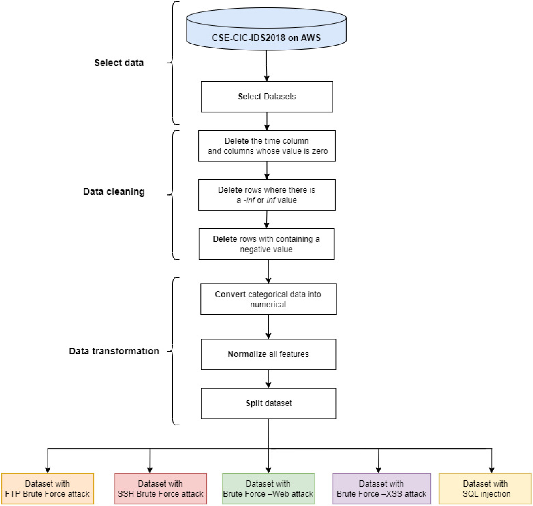

For the current analysis, the time parameter is not needed, nor are the columns where all values are zero since they do not influence the output, i.e. the value of the last column. The data cleaning step resulted in 69 remaining columns after deleting 11 columns out of the original 80 ones. The next step was to delete rows containing invalid values. Therefore, first, the rows with the values inf and $-\textit{inf}$ were deleted, and then rows with negative values in the dataset were also deleted. With these operations, the cleaning of the dataset was completed.

3.3 Data transformation

In course of this research, the data transformation phase comprised three operations, i.e. the transformation of categorical data into numerical, normalization, and splitting of the dataset. To perform further calculations, all non-numerical elements of the dataset were converted into numbers. It was carried out in the case of each categorical column by assigning a number to each category. For example, each occurrence of the string “FTP-BruteForce” was replaced by the value 1. The order of the values was determined arbitrarily not taking into consideration any conceptual distance metrics mainly because later on the dataset was split into subsets containing only data corresponding to one attack type and normal traffic.

Data normalization is a common practice in machine learning, which consists of converting numeric columns to a common scale. In machine learning, some feature values are several times greater than others. Thus the features with higher values could dominate the learning process. However, it does not mean that these variables are more important in predicting the model output. Data normalization converts multiple scaled data to the same scale. After normalization, all variables have similar scale-related effects on the model, which improves the stability and performance of the learning algorithm. There are several types of normalization techniques. The simplest and most used type is the min-max scaling Eq. (1), which rescales a feature into the fixed range [0,1] by subtracting the minimum value of the feature ( $x_{\textit{min}}$ ) from the current value ( $x$ ) and then dividing the result by the range.

$\displaystyle X_{\textit{new}}=\frac{x-x_{\textit{min}}}{x_{\textit{max}}-x_{% \textit{min}}}$ (1)

As a final step in the preprocessing, the selected datasets were split so that each resulting file contained only records corresponding to one attack type as well as records describing normal traffic. This operation resulted in five data files (see Fig. 1). Some of their features are presented in Table 5.

Table 5

Datasets generated during preprocessing

File name	Number of rows	Number of columns
dataset-ftp.csv	857,162	69
dataset-ssh.csv	851,397	69
dataset-web.csv	2085,515	69
dataset-xss.csv	2,085,134	69
dataset-sql.csv	2,084,991	69

3.4 Data reduction

The data reduction phase focuses on feature selection and dimensionality reduction, which can provide several advantages. One of the most important benefits is that many data mining algorithms work better when the number of dimensions – the number of attributes (columns) in the data – is smaller. This is partly because dimensionality reduction eliminates irrelevant attributes and reduces noise. Another advantage is that it can lead to a more comprehensible model because there will be fewer features in it. In addition, the reduced amount of data requires less storage space and less time for its processing.

There are many software tools that can be used to preprocess and analyze large datasets (e.g. Matlab, SPSS, Orange, Python). In the course of this research, we opted for the usage of the Python programming language because it is free of charge and its modules and libraries can produce fast and efficient results. The applied methods and the obtained results are presented in the next section.

4. Feature selection

Feature selection focuses on finding the most relevant attributes, which can be used to carry out an effective classification or prediction [37, 38, 39]. It contributes to the reduction of the dimensionality of the problem and so to the decrease of the resource requirements (storage, computation) as well as it can improve the performance of machine learning algorithms [40], i.e. faster training reduced over-fitting, and sometimes better prediction power. Although this approach may seem to lead to loss of information, this is not the case when redundant or irrelevant information is present. Redundant features are copies of most or all of the information found in one or more other attributes or they can be obtained as a combination of other features.

Irrelevant attributes contain almost no information that is useful for the data mining task to be performed. Redundant and irrelevant features can reduce the accuracy of the classification and the quality of the clusters discovered. While some irrelevant and redundant attributes can be removed immediately by common sense or professional knowledge, the selection of the best subset of at-tributes often requires a systematic approach.

The ideal approach to feature selection is trying all possible subsets of features as input to the data mining algorithm used and then selecting the subset that produced the best results. However, this technique would require an enormous amount of time and computational power. Therefore, several other methods have been developed for this purpose primarily based on statistical assumptions. There are three basic approaches to feature selection.

Wrapper methods: the feature selection algorithm uses the learning method as a subroutine with the computational burden of invoking the learning algorithm to evaluate each subset of features. It finds the best feature set for a given type of machine learning algorithm.

Embedded methods: the machine learning algorithm decides what attributes to use and what features to ignore.

Filter methods: the features are selected before the data mining algorithm is run, using a method that is independent of the data mining task.

Table 6
Strengths and weaknesses of FS techniques

Methods	Advantages	Disadvantages
Wrapper	The performance of the current model is used to select the features, so that the specificities of the model are better taken into account.	Computational demand is high. Risk of over-learning. They are specific to a particular model or algorithm type, so not always generalizable to other problems.
Embedded	Algorithms already include feature selection, avoiding the extra step. They tend to notice complex relationships between features and the target variable.	They tend to increase the complexity of the model, which can lead to over-learning. May require computational resources due to the complexity of the algorithms.
Filter	They are quick to implement as they do not require iterative model training. They do not require prior information about the model or features. Tests correlation.	Do not take into account model specificity and complexity. Correlation-based methods can sometimes select features that have no real relationship to the target property.

All the feature selection methods presented in the next subsections and used in course of this investigation belong to the group of filter methods. Their advantage is that their time complexity is the lowest among the three groups, and usually, after their application, the machine learning algorithm is less prone to over-fitting.

When performing feature selection for machine learning tasks, the goal is to identify the most relevant features that contribute the most information to the target variable. Features with high mutual information are those that are closely related to the target variable and contain valuable information for making predictions. While mutual information (MI) is a valuable metric for feature selection and has several advantages, it also has some limitations that one should be aware of.

Assumption of Independence: Mutual information assumes that the relationship between variables is purely probabilistic and does not consider the underlying causal structure.

Bias towards Variable Complexity: MI can favor variables with high complexity, even if that complexity doesn’t directly contribute to prediction accuracy. Variables that have more distinct values or categories might have higher MI values, but those values might not necessarily be relevant for the target prediction.

Sensitivity to Variable Discretization: The calculation of MI can be sensitive to how you discretize continuous variables. Different discretization schemes can lead to different MI values, impacting the feature selection process.

Limited to Bivariate Relationships: MI only captures the relationship between two variables at a time (bivariate relationships). It doesn’t account for interactions or dependencies involving more than two variables.

Doesn’t Capture Non-Linear Relationships Well: While MI can capture both linear and non-linear relationships to some extent, it might not be able to fully capture intricate non-linear dependencies between variables.

Ignores Irrelevant Information: MI considers all information in a feature equally, even if some of that information is irrelevant or redundant for the target prediction. This can lead to the inclusion of redundant features.

Sensitive to Sample Size: The effectiveness of MI can be affected by the size of your dataset. In cases of small datasets, MI values might not be reliable indicators of feature relevance.

Domain Knowledge is Needed: Interpretation of MI values requires some domain knowledge. High MI values don’t necessarily guarantee that the selected features will be meaningful or actionable.

Bias in Class Imbalanced Data: In cases where the target classes are imbalanced, MI might be biased towards features that are correlated with the majority class, potentially ignoring features that are relevant for the minority class.

Computational Complexity: Calculating mutual information for large datasets with many features can be computationally intensive.

We tried to combine the advantages of the different feature selection methods by creating an ensemble method that employs feature ranking techniques that can address the problem of redundancy ( Symmetric Uncertainty and ANOVA).

4.1 Information gain

$\displaystyle H(Y)=-\sum p(y)\log_{2}(p(y)),$ (2)

where $p(y)$ is the marginal probability density function for the random variable $Y$ . If the observed values of $Y$ in the training dataset are partitioned according to the values of a second feature $X$ , and the entropy of $Y$ with respect to the partitions induced by $X$ is less than the entropy of $Y$ prior to partitioning, then there is a relationship between features $Y$ and $X$ . Thus the entropy of $Y$ after observing $X$ is

$\displaystyle H(Y|X)=\sum p(x)\sum p(y|x)\log_{2}(p(y|x)),$ (3)

where $p(y|x)$ is the conditional probability of $y$ given $x$ . Given the entropy as a criterion of impurity in a dataset, one can define a measure reflecting additional information about $Y$ provided by $X$ that represents the amount by which the entropy of $Y$ decreases. This measure, an indicator of the dependency between $X$ and $Y$ , is known as information gain Eq. (4).

$\displaystyle IG(X,Y)=H(Y)-H(Y|X)=H(X)-H(X|Y).$ (4)

IG is a symmetrical measure. The method provides an orderly classification of all the features, and then a threshold is required to select a certain number of them according to the order obtained. A weakness of the IG criterion is that it is biased in favor of features with more values even when they are not more informative [41].

4.2 Gain ratio

The information gain method prefers to select attributes having a large number of values, which led to the development of the feature selection method gain ratio (GR) which is a modification of the information gain aiming the decrease its bias. Originally developed for decision trees GR takes the number and size of the branches into account when choosing an attribute. It improves the evaluation given by information gain by taking into account the number of splits in the feature, i.e., how equally they are distributed [42]. GR reflects the relevance of each feature the higher its value is the higher the influence of the feature is. Gain ratio is calculated by Eq. (5)

$\displaystyle\textit{GR}(X,Y)=\frac{\textit{IG}(X,Y)}{\textit{SplitInfo}},$ (5) $\displaystyle\textit{SplitInfo}=-\sum p(i)*\log_{2}(p(i)),$ (6)

where $p(i)$ represents the proportion of instances that fall into a particular split of the feature [43].

4.3 Relief

The Relief method calculates a weight value for each feature ( $W_{j}=$ weight of feature “ $j$ ”) that can be used to estimate the quality or relevance of the feature [44]. The weight vector is initialized with zero values, and it is updated using an iterative approach. The algorithm takes a random sample of $m$ elements from the dataset. In the case of each instance of the sample ( $R_{i}$ ) it searches for the closest instance that belongs to the same class ( $H_{i}$ ) and for the closest instance that belongs to the other class ( $M_{i}$ ). Next, the value of each feature weight is updated by the Eq. (7).

$\displaystyle W_{j}=W_{j}-\frac{D(R_{ij},H_{ij})}{m}+\frac{D(R_{ij},M_{ij})}{m},$ (7)

where $X_{ij}$ is the $j$ th feature of the $i$ th instance (here $X$ can be $R$ , $H$ , or $M$ ). The function $D$ is defined as:

$\displaystyle D(x,y)=\left\{\begin{matrix}0&\textit{if}\>x=y\\ 1&\textit{otherwise}\end{matrix}\right.$ (8)

The shortcoming of Relief is that it does not identify redundant features, and it can be used only in the case of binary classification problems.

4.4 Symmetric uncertainty

Symmetric uncertainty (SU) can be used to calculate the rank of features for feature selection by calculating the relevance between the feature and the class label. A feature with a high SU value gets high importance [45]. SU is calculated by normalizing the double value of IG to the sum of the entropies of the two variables.

$\displaystyle\textit{SU}(X,Y)=\frac{2xIG(X,Y)}{H(X)+H(Y)},$ (9)

where $H(X)$ and $H(Y)$ are the entropy values of variables $X$ and $Y$ , while $IG(X,Y)$ is the information gain related to the variables $X$ and $Y$ , respectively [46].

4.5 Chi-squared

The Chi-squared test is a statistical hypothesis test that measures divergence from the expected distribution if one assumes that the feature occurrence is actually independent of the class value [47]. The higher the value of chi-squared, the more relevant the feature with respect to the class is. Its calculation is based on the Eq. (10) [48].

$\displaystyle\chi^{2}=\sum_{i=1}^{n_{I}}\sum_{j=1}^{n_{c}}\frac{[A_{ij}-\frac{% R_{i}B_{j}}{N}]^{2}}{\frac{R_{i}B_{j}}{N}},$ (10)

where $n_{I}$ is the number of intervals, $n_{c}$ is the number of classes, $N$ is the total number of instances, $A i j$ the number of instances in the interval $i$ and class $j$ , $R i$ denotes the number of instances in the interval $i$ , and $B j$ the number of instances in class $j$ . The Chi-squared test based evaluation was developed for discrete variables. Therefore in the case of continuous features before its application a discretization has to be carried out.

4.6 ANOVA

Analysis of Variance (ANOVA) is a statistical analysis technique used to compare the means of multiple groups to determine if there is a significant difference between them. Similar to the Chi-squared approach a discretization is necessary before its usage [49]. The key idea of ANOVA is to compare the total variance of the data to the variation within the groups and the variation between the groups. The within-group sum of squares (SSW) Eq. (11) measures the variation within the groups. It is defined as

$\displaystyle\textit{SSW}=\sum_{i=1}^{k}[(n_{i}-1)*\textit{SS}(i)],$ (11)

where $n_{i}$ is the number of instances in group $i$ , and $\textit{SS}(i)$ is the variance of group $i$ .

The Sum of Squares between groups (SSB) Eq. (12) measures the variation between the means of the groups. It is defined as

$\displaystyle\textit{SSB}=K*\sum(x-\bar{\bar{x}})^{2}$ (12)

where $K$ is the number of groups, $\bar{x_{i}}$ is the mean of group $i$ , and $\bar{\bar{x}}$ is the mean of all instances.

The total sum of squares (SST) Eq. (13) is

$\displaystyle\textit{SST}=\textit{SSW}+\textit{SSB}$ (13)

The null hypothesis of ANOVA is that all groups have the same mean, i.e., the values of the investigated feature do not have effect on the final class. The alternative hypothesis is that at least one group has a different mean. The null hypothesis is tested by the help of the F-ratio, which is the ratio of SSB to SSW Eq. (14). An F-ratio higher than a threshold value (called critical F-value) indicates that there is a significant difference between the means of the groups, and so the null hypothesis can be rejected.

$\displaystyle F=\textit{SSB/SSW}$ (14)

The critical F-value is that value of the F-distribution, which is defined by the degrees of freedom for the numerator ( $\textit{df}_{\textit{SSB}}=K-1$ and the degrees of freedom for the denumerator ( $\textit{df}_{\textit{SSW}}=N-K$ ). Here $N$ is the number of instances.

4.7 Ensemble feature selection

Individual feature selection methods often express the importance of examined features at varying scales. Consequently, the initial step in an ensemble method that combines these scores is to standardize the values using the Eq. (15).

$\displaystyle R_{i}=\frac{R_{i,o}+R_{i,\textit{min}}}{R_{i,\textit{max}}-R_{i,% \textit{min}}},$ (15)

where $R_{i,o}$ represents the original score determined by the $i$ th feature ranking method, $R_{i,\textit{min}}$ corresponds to the lowest value calculated by that method, and $R_{i,\textit{max}}$ denotes the highest value computed by that method. In the course of our current research, we have selected the arithmetic mean as the aggregation method, as indicated by Eq. (16).

$\displaystyle R_{\textit{ens}}=\frac{R_{\textit{IG}}+R_{\textit{GR}}+R_{% \textit{SU}}+R_{\chi^{2}}+R_{\textit{Re}}+R_{\textit{AN}}}{6},$ (16)

where $R_{\textit{ens}}$ signifies the final score of the feature calculated by the ensemble method.

5. Classification algorithms

Classification methods are used to predict the class of an object instance based on a feature vector. Machine learning-based classification algorithms build models that can learn from labeled datasets and use them to predict the class of new, unseen data points. In this investigation, we used five different classification algorithms representing four main classification groups. These groups are linear models, probabilistic models, tree-based models, and kernel-based models.

Linear models are represented by the Logistic Regression method, which models the probability of a binary outcome using a sigmoid function.

Probabilistic models are represented by the Naive Bayes model, which assumes that the features are independent given the class and uses Bayes’ theorem to compute the posterior probabilities of each class.

Tree-based models are represented by two methods: the Decision Tree method, a non-parametric model that recursively partitions the feature space into a tree structure, and the Random Forest method, an ensemble model that uses multiple decision trees and aggregates their predictions to improve performance.

Kernel-based models are represented by the Support Vector Machine (SVM) method, which maps the input data into a high-dimensional feature space and finds a hyperplane that maximally separates the classes.

The following subsections provide a brief description of the classification algorithms mentioned above.

5.1 Logistic regression

Logistic Regression (LR) is a linear classification method that estimates the probability of a certain instance belonging to a class (e.g. attack). LR belongs to the family of linear methods and is an alternative to discriminant analysis. Its application prerequisites are less strict than those of discriminant analysis [50]. The key idea of Logistic Regression is to calculate a linear combination (see Eq. (17)) of the feature values $X=[x_{1},x_{2},\ldots,x_{n}]$ for each observation instance, using a coefficient vector $A=[a_{0},a_{1},\ldots,a_{n}]$ that is determined during the classifier’s training.

$\displaystyle Z(x)=a_{0}+a_{1}*x_{1}+\ldots+a_{n}*x_{n},$ (17)

To determine the probability of belonging to the attack class (class 1) Logistic Regression applies a sigmoid function to $Z$ that maps $Z$ to the $[0,1]$ interval.

$\displaystyle h(z)=\frac{1}{1+e^{-z}},$ (18)

Finally, the classifier decides the final class of the observation by comparing the resulting probability value $h$ to a threshold value $h_{tr}$ , as shown in Eq. (19).

$\displaystyle C(h)=\left\{\begin{matrix}1&\textit{if}\>h>h_{tr}\\ 0&\textit{otherwise}\end{matrix}\right.$ (19)

The threshold value $h_{tr}$ is determined during the training phase of the classifier.

5.2 Naive Bayes

The Naive Bayes classification method is based on Bayes’ theorem of conditional probability. It determines the predicted class of an $X=[x_{1},x_{2},\ldots,x_{n}]$ observation using the formula

The Naive Bayes classification method is based on Bayes’ theorem of conditional probability. It predicts the class of an observation $X=[x_{1},x_{2},\ldots,x_{n}]$ using the Eq. (20)

$\displaystyle C(x)=\underset{c_{j}\in C}{\arg\max}\>P(c_{j})\prod_{i=1}^{n}P(x% _{i}|c_{j})$ (20)

where $c_{j}$ is the $j$ th class, $x_{i}$ is the value of the $x_{i}$ th feature, $n$ is the number of features, $P(c_{j})$ is the prior probability of class $j$ , and $P(x_{i}|c_{j})$ is the conditional probability of the value of $x_{i}$ given class $c_{j}$ . The prior probability $P(c_{j})$ is estimated by the relative frequency of class $j$ in the training sample.

In the case of categorical features $P(x_{i}|c_{j})$ is estimated by the relative frequency of the value $x_{i}$ among the training sample elements that belong to class $c_{j}$ . In the case of continuous features $P(x_{i}|c_{j})$ is estimated by the value of the probability density function calculated for $x_{i}$ taking into consideration the training sample elements that belong to class $c_{j}$

$\displaystyle P(x_{i}|c_{j})=\frac{1}{\sigma_{i}\sqrt{2\pi}}e^{-\frac{(x_{i}-% \mu_{i})^{2}}{2\sigma^{2}}},$ (21)

where $\mu_{i}$ is the mean value and $\sigma_{i}$ is the standard deviation of the $i$ th feature among the training sample elements taken into consideration.

5.3 Support vector machine

Support Vector Machine (SVM) [51] is a statistically based supervised classification technique that can be used to efficiently handle high-dimensional data. It creates a multi-dimensional hyperplane that separates the two classes in the case of binary classification problems. Multiclass problems are reduced to multiple binary classification problems.

If no simple linear separation can be carried out it transforms the data by using so-called kernel functions that calculate the hyperplane in a higher dimension. The nonlinearity of the hyperplane can also be tuned with the help of the regularization and the gamma parameters. The value of the regularization parameter describes how much one wants to avoid misclassification in the case of training instances. A high value could result in a more complex hyperplane with a small amount of wrongly classified data points if any.

In the case of high gamma values, only training instances close to the hyperplane will be considered in the course of its definition.

5.4 Decision tree

Decision trees offer an easy-to-interpret and visualize tool for classification. They make the decision based on rules inferred from the feature values of the training sample. Each leaf of the tree corresponds to a class label. At each node, only one feature is taken into consideration and no root-to-leaf path contains twice the same feature. A Classification tree may also provide a confidence measure regarding the quality of the classification. The tree is built up from the training sample in a recursive manner [52]. It is an iterative process whereby data is partitioned into partitions and then further partitioned on each branch. The features used at different nodes are selected using statistical methods like Information Gain or Gini Index. If all features are already used and the remaining sample contains instances belonging to more than one class a leaf is created and its class will be decided using a majority vote.

5.5 Random forest

The Random Forest (RF) method [53] was developed to overcome a shortcoming of Decision Trees, i.e., having the tendency to overfit the sample data. RF mitigates this problem by using a statistical technique called bootstrapping, which generates multiple models and combines their results to make a final decision. The main idea behind RF is that by aggregating the predictions of multiple classifiers, the impact of individual errors can be minimized.

In course of Bootstrapping several smaller samples are drawn from the training dataset randomly with replacement. Each sample is used to train a separate classifier. Thus when classifying a new observation its final class prediction is made by aggregating the results given by the individual models. Usually, it is done by applying a majority voting solution.

6. Experimental results

All five datasets contained a very large number of instances (see Table 5). Therefore when creating the training and test samples only a part of the original data was used. The steps of the training-test sample construction are presented in Fig. 2.

Figure 2.

Creation of training and testing datasets.

Both in the case of the FTP and SSH Brute Force attacks training samples contained 20% of the original instances. We applied stratified sampling to ensure that each class (attack and benign traffic) is represented in the sample. Thus the resulting collection of records contained 20% of the attack rows and 20% of the rows describing benign traffic. The sampling was carried out without replacement. The test samples were created in a similar way by choosing records from the remaining datasets so that the resulting collection of data points represented 10% of the original ones. The resulting record numbers are shown in Tables 7 and 8, respectively.

In the case of the Brute Force Web, Brute Force XSS, and SQL Injection attack types the selection process was slightly different owing to the fact that the number of records describing malicious traffic was very small. Therefore in each case, the collection of attack rows was split into two parts, i.e., 70% was used for training and the remaining 30% for test purposes. Next, the training samples were created by adding 20% of the data points belonging to the benign traffic. Finally, the test samples were compiled by adding 10% of the benign traffic record to the attack rows allocated for test purposes. The resulting record numbers are shown in Tables 7 and 8, respectively.

Table 7

Training datasets

File name	Number of rows	Number of columns
dataset-ftp-tr.csv	171,433	69
dataset-ssh-tr.csv	170,280	69
dataset-web-tr.csv	417,332	69
dataset-xss-tr.csv	417,218	69
dataset-sql-tr.csv	417,042	69

Table 8

Test datasets

File name	Number of rows	Number of columns
dataset-ftp-ts.csv	85,716	69
dataset-ssh-ts.csv	85,140	69
dataset-web-ts.csv	208,636	69
dataset-xss-ts.csv	208,598	69
dataset-sql-ts.csv	208,517	69

6.1 Feature selection results

The six feature selection methods presented in the previous section were applied for all five datasets using 30 university lab computers as well as the ELKH cloud services [54]. The feature selection workflow is presented in Fig. 3. All the necessary program elements were implemented in Python [55][56]. Although several tasks were performed in parallel the whole process took more than two months.

In the case of each dataset and each method, the feature score values obtained at the end of the feature selection process were normalized. Next, the final feature score was calculated in the case of each dataset separately as the mean of the normalized scores.

We then took the normalised value of the final characteristic scores for each dataset and calculated the final value using the EFS method with the arithmetic mean (see Eq. 16) of the 6 values for each characteristic. The detailed results can be found in the Appendix in Tables A1–A5.

Finally, five feature ranking threshold values were set starting from 0.35 and increasing by a step of 0.5. In the case of each value, we selected the features whose score was higher than the threshold. The results are presented in Table 9. In the case of each attack type a separate list of relevant features was identified. Each feature is represented by its ordinal value. Each row of the table contains those features whose score was greater or equal to the threshold given in the first cell. Starting from the second column each column represents an attack type.

Having the selected feature groups we continued our investigation by applying different classification methods that will be presented in the following section.

Table 9
Feature selection based on threshold values

Ranking threshold	FTP	SSH	WEB	XSS	SQL
0.35	02, 17, 19, 35, 00, 44, 56, 59	00, 02, 17, 19, 57, 56, 59	16, 20, 10, 49, 66, 67, 35, 38, 56, 64, 34, 27, 07, 09, 11, 14, 15, 50, 25, 60, 62, 02, 17, 19, 37, 63, 06, 33, 55, 18, 58, 04, 05, 53, 54, 03, 21, 22, 23, 24, 52, 32, 65, 57	25, 27, 16, 40, 02, 05, 17, 19, 34, 53, 06, 18, 55, 21, 22, 23, 24, 51, 13, 39, 57, 37, 56, 33, 32, 03, 11, 52, 04, 54, 58	39, 43, 47, 10, 15, 05, 26, 53, 56, 25, 02, 17, 19, 35, 16, 18, 27, 28, 34, 06, 23, 30, 55, 29, 21, 22, 24, 57, 37, 11, 14
0.40	44, 56, 59	56, 59	34, 27, 07, 09, 11, 14, 15, 50, 25, 60, 62, 02, 17, 19, 37, 63, 06, 33, 55, 18, 58, 04, 05, 53, 54, 03, 21, 22, 23, 24, 52, 32, 65, 57	02, 05, 17, 19, 34, 53, 06, 18, 55, 21, 22, 23, 24, 51, 13, 39, 57, 37, 56, 33, 32, 03, 11, 52, 04, 54, 58	05, 26, 53, 56, 25, 02, 17, 19, 35, 16, 18, 27, 28, 34, 06, 23, 30, 55, 29, 21, 22, 24, 57, 37, 11, 14
0.45	56, 59	56, 59	02, 17, 19, 37, 63, 06, 33, 55, 18, 58, 04, 05, 53, 54, 03, 21, 22, 23, 24, 52, 32, 65, 57	37, 56, 33, 32, 03, 11, 52, 04, 54, 58	06, 23, 30, 55, 29, 21, 22, 24, 57, 37, 11, 14
0.50	56, 59	59	03, 21 ,22, 23, 24, 52, 32, 65, 57	03, 11, 52, 04, 54, 58	57, 37, 11, 14
0.55	56, 59	59	57	58	11,14

Figure 3.

Feature selection workflow.

6.2 Classifiers

The training and testing of the five classifiers was carried out in Orange 3.34, which is an open-source data visualization, machine learning, and data mining toolkit. It offers a visual programming front-end for interactive data visualization and exploratory, quick qualitative data analysis. Its components are called widgets and they range from simple data visualization, subset selection, and preprocessing to empirical evaluation of learning algorithms and predictive modeling. Visual programming is implemented through an interface in which workflows are created by linking predefined or user-designed widgets, while advanced users can use Orange as a Python library for data manipulation and widget alteration. Orange uses common Python open-source libraries for scientific computing, such as numpy, scipy, and scikit-learn, while its graphical user interface operates within the cross-platform Qt framework.

The classifier training and testing workflow used in course of the investigation is shown in Fig. 4. It was carried out separately for each attack type and for each relevant feature collection. For example, in the case of the FTP Brute Force attack and the 0.40 ranking threshold value three features (44, 56, and 59) were supposed to play a significant role. Thus in total 21 workflow executions were necessary and 105 classifiers were trained.

Figure 4.

Classifier training and testing workflow.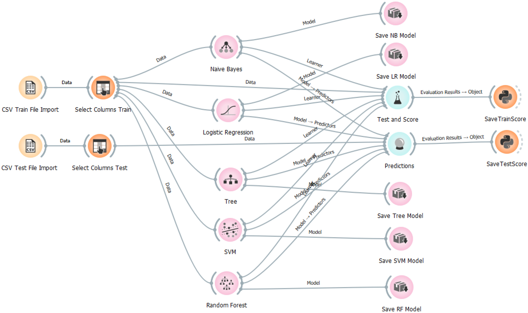

All the classifiers were evaluated against the training and test samples using four measures, i.e., accuracy, precision, recall, and F1. The goal of a binary classifier is to classify input data into one of two possible categories or classes. The goal of the training process is to produce a classifier able to do correct classification not only for the cases used for its training but also for new, different examples. Each example in the training dataset has a label (classification label) that indicates its class. The performance of the classification algorithms is evaluated based on the occurrence number of the four cases presented in Table 10.

Table 10

Classification cases

Label value	Classification value	Case
0	0	TN
0	1	FP
1	0	FN
1	1	TP

The possible cases:

True Positive (TP): it occurs when an attack is categorized as attack.

False Positive (FP): it occurs when the classifier categorizes benign traffic data as an attack.

True Negative (TN): it occurs when the classifier categorizes correctly benign traffic as benign.

False negative (FN): it occurs when the classifier incorrectly identifies an attack as benign traffic.

All classifiers were evaluated on the basis of train and test samples using four measures, i.e. Accuracy, Precision, Recall and F1, which can be calculated using the following equations.

$\displaystyle\textit{Accuracy}=\frac{\textit{TP}+\textit{TN}}{\textit{TP}+% \textit{TN}+\textit{FN}+\textit{FP}}$ (22) $\displaystyle\textit{Precision}=\frac{\textit{TP}}{\textit{TP}+\textit{FP}}$ (23) $\displaystyle\textit{Recall}=\frac{\textit{TP}}{\textit{TP}+\textit{FN}}$ (24) $\displaystyle\textit{F1}=\frac{2(\textit{Precision}\cdot\textit{Recall)}}{% \textit{Precision}+\textit{Recall}}$ (25)

The detailed results can be found in the Appendix in Tables A6–A11.

6.3 Evaluation of results

This section presents the evaluation of the classifiers. Their accuracy is visualized using 3D column charts. In case of each figure the horizontal axis (x) corresponds to the classifier algorithm types, the vertical axis (y) shows the achieved accuracy value, with a maximum value of 1 (best achievable accuracy), and the z axis shows the number of features used for the training of the classifier.

Figure 5.

Accuracy values in case of the FTP attack and the training dataset.

Figure 6.

Accuracy values in case of the FTP attack and the test dataset.

Figure 7.

Accuracy values in case of the SSH attack and the training dataset.

Figure 8.

Accuracy values in case of the SSH attack and the test dataset.

Figure 9.

Accuracy values in case of the WEB attack and the training dataset.

Figure 10.

Accuracy values in case of the WEB attack and the test dataset.

Figure 11.

Accuracy values in case of the XSS attack and the training dataset.

Figure 12.

Accuracy values in case of the XSS attack and the test dataset.

Figure 13.

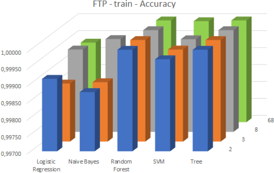
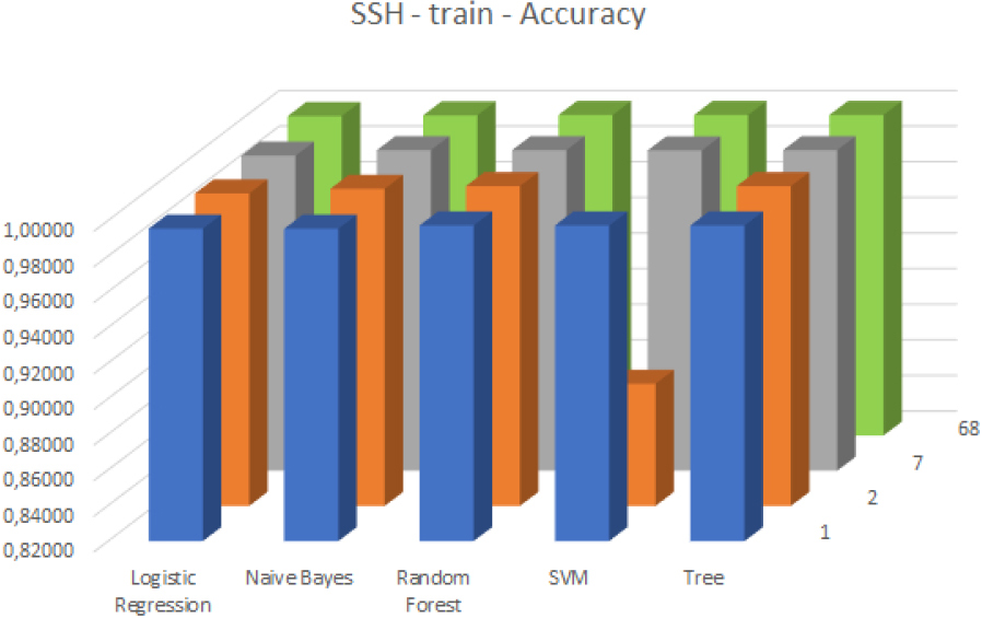
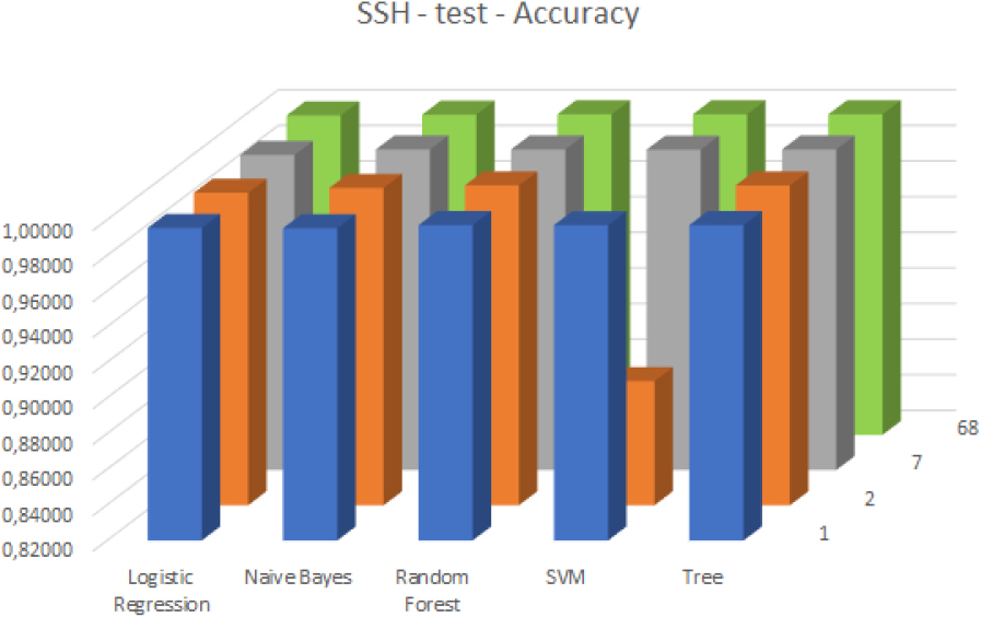
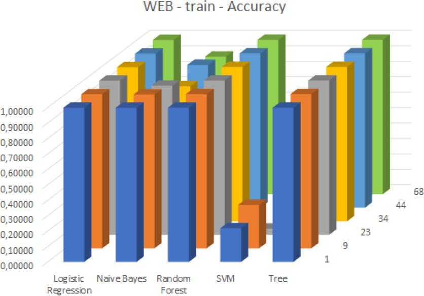
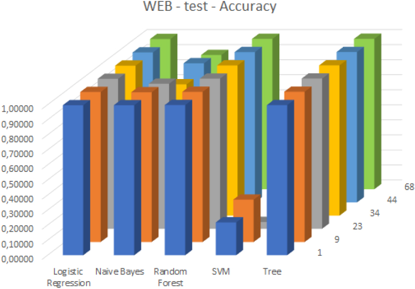
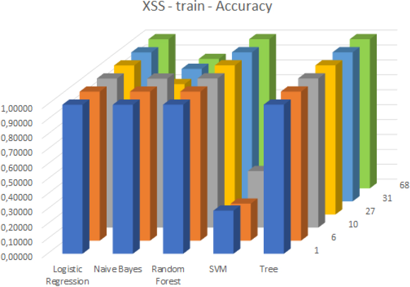
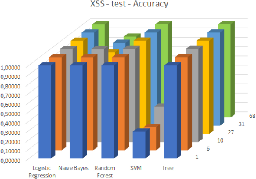
Accuracy values in case of the SQL attack and the training dataset.

Figure 14.

Accuracy values in case of the SQL attack and the test dataset.

In the case of FTP attacks, each of the classifiers performed quite well having high accuracy values and the highest possible recall rates for almost all of the feature subset-classifier type pairs. Except for the case of the logistic regression-based classifier, the accuracy against the training dataset usually improved with increasing the number of selected features (see Fig. 5). However, when evaluating the classifiers with the test dataset a slight decay in accuracy performance could be measured in the case of Naive Bayes and Random Forest classifiers as well (see Fig. 6).

The classifiers also exhibited strong performance against SSH attacks, with high accuracy observed for all feature subset-classifier pairs. Increasing the number of selected features led to improved accuracy against the training dataset, except in the case of the SVM-based classifier (see Fig 7). When evaluating the classifiers against the test dataset revealed a very similar behavior (see Fig 8).

In the case of Web attacks, the SVM classifier provided a low accuracy rate compared to the others both in the case of the training (see Fig. 9) and test (see Fig. 10) datasets. However, Logistic regression, Random Forest, and Decision Tree based classifiers were able to successfully predict the nature of the traffic with a very high accuracy rate. Although the Naive Bayes model in the case of 23 and 34 selected features showed a declining performance its results were not too much fallen behind.

Among the classifiers tested for XSS attacks, the SVM classifier had a low accuracy rate for both the training dataset (see Fig.11) and test dataset (see Fig.12) in comparison to others. The Logistic Regression, Random Forest, and Decision Tree based classifiers performed exceptionally well with a very high accuracy rate. While the Naive Bayes model showed declining performance in the case of 27 and 31 selected features, its results were still competitive.

For SQL Injection attacks, four of the five classifier models demonstrated high accuracy rates against both the training dataset (see Fig. 13) and test dataset (see Fig. 14). The Naive Bayes model was the only exception, showing slightly declining performance when using 26 and 31 selected features, but still having accuracy values over 0.9.

The best-performing classifiers along with ranking threshold values and selected feature number as well as the evaluation results are highlighted in Table 11.

Table 11

Best performing classifiers

Attack type	Ranking treshold	Features	Classifier	Accuracy	Precision	Recall	F1
FTP	0	68	Random Forest	1.00000	1.00000	1.00000	1.00000
	0.35	8	Random Forest	1.00000	1.00000	1.00000	1.00000
SSH	0	68	Random Forest	0.99999	0.99997	1.00000	0.99999
	0.35	7	Random Forest	0.99999	0.99997	1.00000	0.99999
WEB	0	68	Tree	0.99995	0.99165	0.97218	0.98182
	0.35	44	Tree	0.99994	0.98997	0.96890	0.97932
XSS	0	68	Tree	0.99999	0.99561	0.98696	0.99127
	0.45	10	Random Forest	0.99999	1.00000	0.97391	0.98678
SQL	0	68	Tree	1.00000	1.00000	0.97701	0.98837
	0.40	26	Tree	0.99999	1.00000	0.95402	0.97647

7. Conclusions

In course of the investigation reported this paper, six feature evaluation techniques were performed on five datasets after completing the data cleaning and transformation steps. Each dataset comprised records that described two types of traffic cases: benign and attack, and featured 69 attributes. An average score was calculated after normalization and used to rank individual features. Next, six ranking thresholds were defined, which led to the selection of several relevant feature collections for each attack type. The number of included attributes varied widely, ranging from 1 (SSH) to 44 (Web).

Next, five classifier models were trained for each collection using the Orange software tool, and their performance was evaluated against the train and test datasets using four classification metrics. It was observed that, in some cases, accuracy improved slightly when increasing the number of features. However, excellent results were achieved in most cases, even with a low number of attributes. Table 11, which shows the best-performing classifiers for each attack type, clearly indicates that no general threshold can be set for the feature scores. The results suggest that tree-type classification algorithms represent the most appropriate solution for the investigated attack types when feature selection followed the presented workflow.

The methodology utilized in the current investigation can be applied to other scenarios involving high-dimensional data, such as clustering (e.g. [57, 58]), object identification [59], classification [60], indor localization [61], or technology optimization [62].

Examining network communication (including normal and attack cases) with the help of the ensemble feature selection method, actual data and information can be configured for the sensors of an IDS system for certain types of attacks with the help of the features included in the defined feature groups. From the network communication data with originally 80 characteristics, only the groups of the selected characteristics need to be taken into account in order to achieve a good classification result for an IDS to detect the appropriate attacks. There are IDS software that can be configured at a professional level, such as Suricata. The code provided to integrate machine learning features into Suricita consists of two parts: the Suricata source files and the new classification scripts with associated configuration files [63].

Further research will focus on the investigation of the suitability of different aggregation techniques (e.g. [64, 65]) that could replace the average score in feature relevance calculation. Furthermore the applicability of further computational intelligence methods.

Footnotes

Acknowledgments

On behalf of the project we are grateful for the possibility to use ELKH Cloud []; (https://science-cloud.hu/), which helped us achieve the results published in this paper.

This research was supported by 2020-1.1.2-PIACI-KFI-2020-00062 “Development of an industrial 4.0 modular industrial packaging machine with integrated data analysis and optimization based on artificial intelligence, error analysis”. The Hungarian Government supports the Project and is co-financed by the European Social Fund.

Author contributions

Conceptualisation, L.G. and Z.C. J.; formal analysis, L.G. and Z.C. J.; Funding acquisition, L.G. and Z.C. J.; investigation, L.G. and Z.C. J.; methodology, L.G. and Z.C. J.; Writing-review & editing, L.G. and Z.C. J.; supervision, L.G. and Z.C. J. All authors have read and agreed to the published version of the manuscript.

References

Göcs

and Johanyák

Z.C.

, Survey On Intrusion Detection Systems, in: 7th International Scientific and Expert Conference TEAM 2015 Technique, Education, Agriculture & Management, 2015.

Göcs

Johanyák

Z.C.

and Kovács

, Review of Anomaly-Based IDS algorithms, in: 8th International Scientific and Expert Conference TEAM 2016 Technique, Education, Agriculture & Management, 2016.

Pes

, Ensemble feature selection for high-dimensional data: a stability analysis across multiple domains, Neural Computing and Applications 32(10) (2020), 5951–5973. doi: 10.1007/s00521-019-04082-3.

Chen

Wang

Lan

et al., CNFRD: A Few-Shot Rumor Detection Framework via Capsule Network for COVID-19, International Journal of Intelligent Systems 2023 (2023). doi: 10.1155/2023/2467539.

Lyu

Feng

and Sakurai

, A survey on feature selection techniques based on filtering methods for cyber attack detection, Information 14(3) (2023), 191. doi: 10.3390/info14030191.

Venkatesan

, Design an Intrusion Detection System based on Feature Selection Using ML Algorithms, Mathematical Statistician and Engineering Applications 72(1) (2023), 702–710.

Thakkar

and Lohiya

, Fusion of statistical importance for feature selection in Deep Neural Network-based Intrusion Detection System, Information Fusion 90 (2023), 353–363. doi: 10.1016/j.inffus.2022.09.026.

Ullah

Srivastava

and Lin

J.C.-W.

, IDS-INT: Intrusion detection system using transformer-based transfer learning for imbalanced network traffic, Digital Communications and Networks (2023). doi: 10.1016/j.dcan.2023.03.008.

Stiawan

Idris

M.Y.B.

Bamhdi

A.M.

Budiarto

et al., CICIDS-2017 dataset feature analysis with information gain for anomaly detection, IEEE Access 8 (2020), 132911–132921. doi: 10.1109/ACCESS.2020.3009843.

10.

Rahman

M.A.

Asyhari

A.T.

Wen

O.W.

Ajra

Ahmed

and Anwar

, Effective combining of feature selection techniques for machine learning-enabled IoT intrusion detection, Multimedia Tools and Applications 80(20) (2021), 31381–31399. doi: 10.1007/s11042-021-10567-y.

11.

Javadpour

Abharian

S.K.

and Wang

, Feature selection and intrusion detection in cloud environment based on machine learning algorithms, in: 2017 IEEE international symposium on parallel and distributed processing with applications and 2017 IEEE international conference on ubiquitous computing and communications (ISPA/IUCC), IEEE, 2017, pp. 1417–1421. doi: 10.1109/ISPA/IUCC.2017.00215.

12.

Taher

K.A.

Jisan

B.M.Y.

and Rahman

M.M.

, Network intrusion detection using supervised machine learning technique with feature selection, in: 2019 International conference on robotics, electrical and signal processing techniques (ICREST), IEEE, 2019, pp. 643–646. doi: 10.1109/icrest.2019.8644161.

13.

Kocher

and Kumar

, Analysis of machine learning algorithms with feature selection for intrusion detection using UNSW-NB15 dataset, Available at SSRN 3784406 (2021). doi: 10.5121/ijnsa.2021.13102.

14.

Alkasassbeh

, An empirical evaluation for the intrusion detection features based on machine learning and feature selection methods, arXiv preprint arXiv:1712.09623 (2017). doi: 10.48550/arXiv.1712.09623.

15.

Thaseen

I.S.

and Kumar

C.A.

, Intrusion detection model using fusion of chi-square feature selection and multi class SVM, Journal of King Saud University-Computer and Information Sciences 29(4) (2017), 462–472. doi: 10.1016/j.jksuci.2015.12.004.

16.

Awotunde

J.B.

Chakraborty

and Adeniyi

A.E.

, Intrusion detection in industrial internet of things network-based on deep learning model with rule-based feature selection, Wireless Communications and Mobile Computing 2021 (2021). doi: 10.1155/2021/7154587.

17.

Sasan

H.P.S.

and Sharma

, Intrusion detection using feature selection and machine learning algorithm with misuse detection, International Journal of Computer Science and Information Technology 8(1) (2016), 17–25. doi: 10.5121/ijcsit.2016.8102.

18.

Biswas

S.K.

et al., Intrusion detection using machine learning: A comparison study, International Journal of Pure and Applied Mathematics 118(19) (2018), 101–114.

19.

Ali

Shaukat

Tayyab

Khan

M.A.

Khan

J.S.

Ahmad

et al., Network intrusion detection leveraging machine learning and feature selection, in: 2020 IEEE 17th International Conference on Smart Communities: Improving Quality of Life Using ICT, IoT and AI (HONET), IEEE, 2020, pp. 49–53. doi: 10.1109/honet50430.2020.9322813.

20.

Malhotra

Sharma

et al., Intrusion detection using machine learning and feature selection, International Journal of Computer Network and Information Security 11(4) (2019), 43. doi: 10.5815/ijcnis.2019.04.06.

21.

Krishnaveni

Sivamohan

Sridhar

and Prabakaran

, Efficient feature selection and classification through ensemble method for network intrusion detection on cloud computing, Cluster Computing 24(3) (2021), 1761–1779. doi: 10.1007/s10586-020-03222-y.

22.

Kumar

and Batth

J.S.

, Network intrusion detection with feature selection techniques using machine-learning algorithms, International Journal of Computer Applications 150(12) (2016). doi: 10.5120/ijca2016910764.

23.

Pattawaro

and Polprasert

, Anomaly-based network intrusion detection system through feature selection and hybrid machine learning technique, in: 2018 16th International Conference on ICT and Knowledge Engineering (ICT&KE), IEEE, 2018, pp. 1–6. doi: 10.1109/ictke.2018.8612331.

24.

Ahmad

and Aziz

M.N.

, Data preprocessing and feature selection for machine learning intrusion detection systems, ICIC Express Lett 13(2) (2019), 93–101. doi: 10.24507/icicel.13.02.93.

25.

Aggarwal

and Sharma

S.K.

, Analysis of KDD dataset attributes-class wise for intrusion detection, Procedia Computer Science 57 (2015), 842–851. doi: 10.1016/j.procs.2015.07.490.

26.

Basnet

R.B.

Shash

Johnson

Walgren

and Doleck

, Towards Detecting and Classifying Network Intrusion Traffic Using Deep Learning Frameworks., J. Internet Serv. Inf. Secur. 9(4) (2019), 1–17.

27.

Sharafaldin

Lashkari

A.H.

and Ghorbani

A.A.

, Toward generating a new intrusion detection dataset and intrusion traffic characterization, ICISSp 1 (2018), 108–116. doi: 10.5220/0006639801080116.

28.

Chen

Ghorbani

A.A.

et al., A survey on user profiling model for anomaly detection in cyberspace, Journal of Cyber Security and Mobility 8(1) (2019), 75–112. doi: 10.13052/jcsm2245-1439.814.

29.

Sharafaldin

Gharib

Lashkari

A.H.

and Ghorbani

A.A.

, Towards a reliable intrusion detection benchmark dataset, Software Networking 2018(1) (2018), 177–200. doi: 10.13052/jsn2445-9739.2017.009.

30.

Ring

Wunderlich

Grüdl

Landes

and Hotho

, Creation of flow-based data sets for intrusion detection, Journal of Information Warfare 16(4) (2017), 41–54.

31.

Ring

Wunderlich

Grüdl

Landes

and Hotho

, Flow-based benchmark data sets for intrusion detection, in: Proceedings of the 16th European Conference on Cyber Warfare and Security. ACPI, 2017, pp. 361–369.

32.

Moustafa

and Slay

, UNSW-NB15: a comprehensive data set for network intrusion detection systems (UNSW-NB15 network data set), in: 2015 military communications and information systems conference (MilCIS), IEEE, 2015, pp. 1–6. doi: 10.1109/MilCIS.2015.7348942.

33.

Moustafa

and Slay

, The evaluation of Network Anomaly Detection Systems: Statistical analysis of the UNSW-NB15 data set and the comparison with the KDD99 data set, Information Security Journal: A Global Perspective 25(1–3) (2016), 18–31. doi: 10.1080/19393555.2015.1125974.

34.

Maciá-Fernández

Camacho

Magán-Carrión

García-Teodoro

and Therón

, UGR’16: A new dataset for the evaluation of cyclostationarity-based network IDSs, Computers & Security 73 (2018), 411–424. doi: 10.1016/j.cose.2017.11.004.

35.

Bhuyan

M.H.

Bhattacharyya

D.K.

and Kalita

J.K.

, Towards Generating Real-life Datasets for Network Intrusion Detection., Int. J. Netw. Secur. 17(6) (2015), 683–701.

36.

Lashkari

A.H.

Draper-Gil

Mamun

M.S.I.

Ghorbani

A.A.

et al., Characterization of tor traffic using time based features. (2017), 253–262. doi: 10.5220/0006105602530262.

37.

Muhi

and Johanyák

Z.C.

, Dimensionality reduction methods used in Machine Learning, Műszaki Tudományos Közlemények 13(1) (2020), 148–151. doi: 10.33894/mtk-2020.13.27.

38.

Viharos

Z.J.

Kis

K.B.

Fodor

Á.

and Büki

M.I.

, Adaptive, hybrid feature selection (AHFS), Pattern Recognition 116 (2021), 107932. doi: 10.1016/j.patcog.2021.107932.

39.

Dobján

and Antal

E.D.

, Modern feature extraction methods and learning algorithms in the field of industrial acoustic signal processing, in: 2017 IEEE 15th International Symposium on Intelligent Systems and Informatics (SISY), IEEE, 2017, pp. 000065–000070. doi: 10.1109/sisy.2017.8080589.

40.

Chauhan

N.S.

, Decision Tree Algorithm-Explained, 2020, KDnuggets, [Online]. Available: [Accessed 16 April 2021].

41.

Karegowda

A.G.

Manjunath

and Jayaram

, Comparative study of attribute selection using gain ratio and correlation based feature selection, International Journal of Information Technology and Knowledge Management 2(2) (2010), 271–277.

42.

Priyadarsini

R.P.

Valarmathi

and Sivakumari

, Gain ratio based feature selection method for privacy preservation, ICTACT Journal on Soft Computing 1(4) (2011), 201–205. doi: 10.21917/ijsc.2011.0031.

43.

Pasha

S.J.

and Mohamed

E.S.

, Ensemble gain ratio feature selection (EGFS) model with machine learning and data mining algorithms for disease risk prediction, in: 2020 International Conference on Inventive Computation Technologies (ICICT), IEEE, 2020, pp. 590–596. doi: 10.1109/ICICT48043.2020.9112406.

44.

Urbanowicz

R.J.

Meeker

La Cava

Olson

R.S.

and Moore

J.H.

, Relief-based feature selection: Introduction and review, Journal of Biomedical Informatics 85 (2018), 189–203. doi: 10.1016/j.jbi.2018.07.014.

45.

Singh

Kushwaha

Vyas

O.P.

et al., A feature subset selection technique for high dimensional data using symmetric uncertainty, Journal of Data Analysis and Information Processing 2(4) (2014), 95. doi: 10.4236/jdaip.2014.24012.

46.

Bakhshandeh

Azmi

and Teshnehlab

, Symmetric uncertainty class-feature association map for feature selection in microarray dataset, International Journal of Machine Learning and Cybernetics 11(1) (2020), 15–32. doi: 10.1007/s13042-019-00932-7.

47.

Forman

et al., An extensive empirical study of feature selection metrics for text classification., J. Mach. Learn. Res. 3(Mar) (2003), 1289–1305.

48.

Bolón-Canedo

Sánchez-Maroño

and Alonso-Betanzos

, Feature selection for high-dimensional data, Springer, 2015. ISBN 978-3-319-21857-1. doi: 10.1007/978-3-319-21858-8.

49.

Kumar

Rath

N.K.

Swain

and Rath

S.K.

, Feature selection and classification of microarray data using MapReduce based ANOVA and K-nearest neighbor, Procedia Computer Science 54 (2015), 301–310. doi: 10.1016/j.procs.2015.06.035.

50.

Maalouf

, Logistic regression in data analysis: an overview, International Journal of Data Analysis Techniques and Strategies 3(3) (2011), 281–299. doi: 10.1504/IJDATS.2011.041335.

51.

Steinwart

and Christmann

, Support vector machines, 1st ed edn, Information science and statistics, Springer, New York, 2008. ISBN 978-0-387-77241-7 978-0-387-77242-4.

52.

Charbuty

and Abdulazeez

, Classification based on decision tree algorithm for machine learning, Journal of Applied Science and Technology Trends 2(01) (2021), 20–28. doi: 10.38094/jastt20165.

53.

Breiman

, Random forests, Machine Learning 45 (2001), 5–32. doi: 10.1023/A:1010933404324.

54.

Héder

Rigó

Medgyesi

Lovas

Tenczer

Török

Farkas

Emődi

Kadlecsik

Mező

Pintér

Á.

and Kacsuk

, The Past, Present and Future of the ELKH Cloud, Információs Társadalom 22(2) (2022), 128. doi: 10.22503/inftars.xxii.2022.2.8.

55.

Bernard

and Bernard

, Python data analysis with pandas, Python Recipes Handbook: A Problem-Solution Approach (2016), 37–48.

56.

McKinney

et al., Data structures for statistical computing in python, in: Proceedings of the 9th Python in Science Conference, Vol. 445, Austin, TX, 2010, pp. 51–56.

57.

Blažič

and Škrjanc

, Incremental fuzzy c-regression clustering from streaming data for local-model-network identification, IEEE Transactions on Fuzzy Systems 28(4) (2019), 758–767. doi: 10.1109/TFUZZ.2019.2916036.

58.

Borlea

I.-D.

Precup

R.-E.

Borlea

A.-B.

and Iercan

, A unified form of fuzzy C-means and K-means algorithms and its partitional implementation, Knowledge-Based Systems 214 (2021), 106731. doi: 10.1016/j.knosys.2020.106731.

59.

Hvizdoš

Vaščák

and Brezina

, Object identification and localization by smart floors, in: 2015 IEEE 19th International Conference on Intelligent Engineering Systems (INES), IEEE, 2015, pp. 113–117. doi: 10.1109/INES.2015.7329649.

60.

Duer

Pokoradi

Bernatowicz

and Duer

, Classification of elements in the diagnostic model of a technical object for building an expert knowledge base, Journal of Mechanical and Energy Engineering 1(1), (2017), 71–78.

61.

Vincze

and Niitsuma

, What-You-See-Is-What-You-Get Indoor Localization for Physical Human-Robot Interaction Experiments, in: 2022 IEEE/ASME International Conference on Advanced Intelligent Mechatronics (AIM), 2022, pp. 909–914. doi: 10.1109/AIM52237.2022.9863359.

62.

Babič

Karabegović

Martinčič

S.I.

and Varga

, New method of sequences spiral hybrid using machine learning systems and its application to engineering, in: New Technologies, Development and Application 4, Springer, 2019, pp. 227–237. doi: 10.1007/978-3-319-90893-9_28.

63.

Coscia

, Smart intrusion detection systems based on machine learning, PhD thesis, Politecnico di Torino, 2021.

64.

Lilik

Bukovics

Á.

and Kóczy

L.T.

, Fuzzy Inference System-like Aggregation Operator for Fuzzy Signatures, in: Computational Intelligence and Mathematics for Tackling Complex Problems 4, Springer, 2022, pp. 93–101. doi: 10.1007/978-3-031-07707-4_12.

65.

Tóth-Laufer

and Takács

, The effect of aggregation and defuzzification method selection on the risk level calculation, in: 2012 IEEE 10th International Symposium on Applied Machine Intelligence and Informatics (SAMI), IEEE, 2012, pp. 131–136. doi: 10.1109/SAMI.2012.6208943.

Identifying relevant features of CSE-CIC-IDS2018 dataset for the development of an intrusion detection system

Abstract

Keywords

1. Introduction

2. Related works

Table 1 Summary of related works

3.1 Datasets

Table 2 IDS datasets

4. Feature selection

Table 6 Strengths and weaknesses of FS techniques

5.1 Logistic regression

5.4 Decision tree

5.5 Random forest

6. Experimental results

Table 9 Feature selection based on threshold values

Footnotes

Acknowledgments

Author contributions

References

Table 1
Summary of related works

Table 2
IDS datasets

Table 6
Strengths and weaknesses of FS techniques

Table 9
Feature selection based on threshold values