ATIN: Attention-embedded time-aware imputation networks for production data anomaly detection

Abstract

Effective identification of anomalous data from production time series in the oilfield affects future analysis and forecasting. Such time series is often characterized by irregular time intervals due to uneven manual sampling, and missing values caused by incomplete measurements. Therefore, the identification task becomes more challenging. In this paper, an Attention-Embedded Time-Aware Imputation Network (ATIN) with two sub-networks is proposed for this task. First, Time-Aware Imputation LSTM (TI-LSTM) is designed for modeling irregular time intervals and incomplete measurements. It decays the long-term memory component as the producing well conditions may be varied during the water cut stage. Second, Attention-Embedding LSTM (ATEM) is designed to improve the effectiveness of anomaly detection. It focuses on the correlation between the last and historical measurements in a given sequence. Comparison experiments with several state-of-the-art methods, including mTAN, GRU-D, T-LSTM, ATTAIN, and BRITS are conducted. Results show that the proposed ATIN performs better in accuracy, $F_{1}$ -score, and area under curve (AUC).

Keywords

Attention mechanism missing value production data time series

1. Introduction

The petroleum industry generates a large amount of data such as seismic, core, and production data [1, 2]. The application of neural network methods in the petroleum industry has been widely explored [3, 4, 5, 6]. However, reality factors such as equipment quality, bad weather, and human activities can cause unreliability of data [7]. Therefore, an important task is to predict whether to adopt newly generated production data, especially fluid rate, and water cut, based on historical data from producing wells. Accurate predictions help oilfield management to schedule effective production measures [8].

This task is challenging because the oil well production data is an irregular multivariate time series (IMTS [9]) with many missing values and varying intervals. The production data of a producing well is shown in Fig. 1. The sampling of data by oilfield workers is irregular. For producing well data, there is a time gap of either two or three days between the first and second measurements. In addition, the data measured each time may be incomplete, and staff often only measure some of the characteristics. Uneven and incomplete measurement of data is the key challenge of this task.

Figure 1.

Production data of a producing well. Three features of pump frequency, fluid rate, and water cut are shown. The three enlarged graphs framed by dashed lines show that the intervals between sampling points are heterogeneous. Furthermore, it should be noted that not all features were recorded at every time point.

Machine learning, particularly neural networks, has exhibited notable success in modeling oil production time series. Among these approaches, the artificial neural network (ANN) has been widely employed for successful oil production prediction [10, 11, 12, 3]. Nevertheless, a more effective strategy involves the utilization of recurrent neural networks (RNNs) to handle such data [13, 14]. Remarkably, [13] reported experimental results demonstrating the superior performance of the LSTM (Long Short-Term Memory) [15] over ANN. Furthermore, studies conducted by [16, 17] show that bidirectional GRUs exhibit superior performance compared to other unidirectional RNNs. However, it is worth noting that they all assume uniform sampling data without any missing values.

Recently, many deep learning methods focus on IMTS. One approach is using IMTS RNNs (RNNs for IMTS). GRU-D [18] inputs missing values by combining the mean and last observation and capturing irregular time-interval of features using a trainable decay mechanism. However, the imputation method of fixing missing values has limitations, which assumes that the data must tend to maintain past and mean values. T-LSTM [19] decays the short-term memory in the cell state of LSTM and retains the long-term memory, so that it is more prepared to capture the irregular time interval characteristics of a specific sequence, but it does not deal with missing values. Brits [20] simply regresses the hidden layer of RNNs to estimate the data at the next time point, completing the imputation without any specific assumptions. ATTAIN [21] simultaneously utilizes the decay function and attention mechanism to capture the time interval irregularity and global characteristics of sequence data. The decay function of FT-LSTM [22] superimposes three subfunctions representing convex, linear, and concave to increase its flexibility and generality. These RNNs perform well in modeling IMTS. While these methods do not address both irregular sampling and incomplete measurement problems.

Some approaches use attention mechanisms to model IMTS [23, 24, 25]. Like [26], most of these methods learn a time representation and then use the attention mechanism to model sequences. One noteworthy approach is mTAN [27] which only uses the time embedding. It takes irregularly sampled time points and the corresponding values as keys and values, and produces a fixed dimensional representation at the query time points. Building upon mTAN, UnTAN [28] further models the heteroskedasticity of the sequence based on mTAN. However, the production process of a producing well built on complex mechanics [14, 13] is non-repeatable. Using time embedding to get attention weights limits the expressiveness of the model. ATTAIN [21] and MCE [29] also use attention mechanisms. However, instead of encoding time, they put it into a time-aware mechanism as a more intuitive representation of the positional relationships in the sequence.

Apart from approaches based on IMTS RNNs and attention mechanisms, recent advancements have introduced methods grounded in neural ordinary differential equations (ODEs) [30] for establishing continuous dynamics relationships between hidden states of two observations. Nonetheless, the solution of an ODE is primarily determined by its initial conditions, lacking a mechanism to adapt the trajectory based on subsequent observations. GRU-ODE Bayes [31] and ODE-RNN [32] employ RNNs to update the hidden states of novel observations. On the other hand, NJ-ODE [33] assumes that the data is a continuous stochastic process and that the predictions approximate the conditional expectation given the currently available information. Drawing parallels to neural ODEs are neural controlled differential equations (CDEs) [34, 35]. Unlike neural ODEs, the vector field of neural CDEs relies on time-varying data, thereby enabling the system trajectory to be influenced by a sequence of observations. While neural ODEs are elegant network models, their reliance on numerical ODE solvers often results in considerably longer training times compared to RNNs [36].

In addition, Generative Adversarial Networks (GANs) [37, 38, 39, 40, 41] with IMTS RNNs as generators are also designed. However, GAN-structured networks have the problem of training difficulties [42]. Some models interpolate data by combining non-deep learning methods (e.g., Gaussian process, Kalman filter) and RNNs [9, 43]. They assume that the data satisfy a Gaussian process or a mutually independent Gaussian distribution.

In this paper, ATIN is proposed for anomalous production data detection. This model does not require any assumptions. The problems of irregular time intervals and incomplete measurement are addressed simultaneously. The downstream task of anomalous production data detection is also handled. It consists of two sub-networks:

•

TI-LSTM is a combination of our modified T-LSTM [19] with RITS-I [20]. It can perform both imputation and time-aware tasks. During production in the water cut stage, the formation physical properties are varied. Meanwhile, experts estimate the fluid rate and water cut based on historical production data from the last one to two weeks. Therefore, the idea behind TI-LSTM is to retain the short-term memory and decay the long-term memory. However, it is difficult for TI-LSTM to focus on the downstream task of detecting anomalous production data since it is mainly used for imputation.

•

ATEM is used for this downstream task, and it has different forward and backward network structures. Its structure is referenced from ATTAIN [21]. It takes the hidden states of TI-LSTM as input so that a two-layer stacked RNN is formed. TI-LSTM is responsible for learning the representation of the points in the production sequence. ATEM is concerned with the correlation between the last point and the rest of the points in the sequence.

Comparative experiments with state-of-the-art methods, including mTAN, GRU-D, T-LSTM, ATTAIN, and BRITS are implemented using a realistic producing well dataset. The results show that ATIN is better to learn the distinguished representation from uneven producing well data with missing values.

The rest of the paper is organized as follows: Problem formulation and some necessary preliminaries are introduced in Section 2, the detailed implementation of our method is presented in Section 3, comparison of the experimental results with other typical methods is presented in Section 4, and the study is concluded in Section 5.

2. Preliminary

The problem formulation and some necessary preliminaries are presented in this section. Table 1 lists the main notations used in this paper.

Table 1
Notations

Notation	Meaning
$\mathbf{T}$	A series of time points
$\mathbf{X}$	Dataset
$\mathbf{M}$	Masking matrix
$\mathbf{y}$	Binary label vector
$\delta$	Time intervals of features
$\mathbf{x}^{c}$	“Complete” input
$\mathbf{h}^{c}$	Decayed hidden state
$\mathbf{c}^{*}$	Adjusted cell state
$\hat{\mathbf{X}}$	Estimates in forward direction
$g_{c}$	Decay function of cell state
$g_{h}$	Decay function of hidden state
$\mathbf{C}$	Accumulated cell state in forward direction
$\mathcal{L}_{e}$	Estimation loss
$\mathcal{L}_{c}$	Consistency loss
$\mathcal{L}_{p}$	Prediction loss
$\alpha$	Attention weight
$\beta$	Focusing parameter
$\gamma$	Weight factor
$\eta$	Prediction threshold
$\lambda$	Loss weigth

2.1 Problem statement

The anomalous production data with missing values is a multivariate time series

$\displaystyle S=(\mathbf{T},\mathbf{X},\mathbf{M},\mathbf{y}),$ (1)

where

•

$\mathbf{T}=(s_{1},s_{2},\dots,s_{n})^{\mathsf{T}}$ is a series of $n$ time points with $s_{i}<s_{i+1}$ for $1\leqslant i\leqslant n-1$ . Note that $s_{i+1}-s_{i}$ is not a constant for different $i$ , indicating uneven time series;

•

$\mathbf{X}=(\mathbf{x}_{1},\mathbf{x}_{2},\dots,\mathbf{x}_{n})^{\mathsf{T}}=(% x_{ij})_{n\times d}\in(\mathbb{R}^{+}\cup\{0\})^{n\times d}$ is the data with $d$ features collected at these time points;

•

$\mathbf{M}=(m_{ij})_{n\times d}\in\{0,1\}^{n\times d}$ is the masking matrix where $m_{ij}=0$ indicating that $x_{ij}$ is missing, and $m_{ij}=1$ indicating a valid value;

•

$\mathbf{y}=(y_{1},y_{2},\dots,y_{n})^{\mathsf{T}}\in\{0,1\}^{n}$ is the binary label vector indicating normal or anomalous data by 0 and 1, respectively.

In many cases, features are continuously missing. For the $j$ -th feature, the interval between the current time point and the last time point with valid value is given by

$\displaystyle\delta_{ij}=\left\{\begin{array}[]{ll}0,&i=1;\\ s_{i}-s_{i-1},&i>1,m_{i-1,j}=1;\\ s_{i}-s_{i-1}+\delta_{i-1,j},&i>1,m_{i-1,j}=0.\\ \end{array}\right.$ (2)

The anomalous detection task is to predict the label of the current time point according to historical and current data. Suppose that the current label is related to at most $k$ recent time points, then this work is to learn a prediction model

$\displaystyle\theta:\mathbf{T}_{i}^{k}\times\mathbf{X}_{i}^{k}\times\mathbf{M}% _{i}^{k}\mapsto\hat{y_{i}},$ (3)

where

•

$\mathbf{T}_{i}^{k}=(s_{i-k+1},s_{i-k+2},\dots,s_{i})$ ;

•

$\mathbf{X}_{i}^{k}=(\mathbf{x}_{i-k+1},\mathbf{x}_{i-k+2},\dots,\mathbf{x}_{i})$ ;

•

$\mathbf{M}_{i}^{k}=(\mathbf{m}_{i-k+1},\mathbf{m}_{i-k+2},\dots,\mathbf{m}_{i})$ .

2.2 Long short-term memory

RNNs, such as LSTM [15] are powerful sequence models. In the standard LSTM cell unit, the cell state $\mathbf{c}_{t}$ is used as internal memory and controls the information flow. It is generated by forgetting information through the forgetting gate $\mathbf{f}_{t}$ and the nearest cell state $\mathbf{c}_{t-1}$ and adding new information through the input gate $\mathbf{i}_{t}$ and the candidate cell state $\mathbf{g}_{t}$ . Finally, the hidden state $\mathbf{h}_{t}$ is generated by filtering the new cell state $\mathbf{c}_{t}$ through the output gate layer $\mathbf{o}_{t}$ . The process of LSTM is as follows:

$\displaystyle\begin{split}&\displaystyle\mathbf{i}_{t}=\sigma(\mathbf{W}_{i}[% \mathbf{x}_{t}\circ\mathbf{h}_{t-1}]+\mathbf{b}_{i}),\\ &\displaystyle\mathbf{f}_{t}=\sigma(\mathbf{W}_{f}[\mathbf{x}_{t}\circ\mathbf{% h}_{t-1}]+\mathbf{b}_{f}),\\ &\displaystyle\mathbf{o}_{t}=\sigma(\mathbf{W}_{o}[\mathbf{x}_{t}\circ\mathbf{% h}_{t-1}]+\mathbf{b}_{o}),\\ &\displaystyle\mathbf{g}_{t}=\tanh(\mathbf{W}_{g}[\mathbf{x}_{t}\circ\mathbf{h% }_{t-1}]+\mathbf{b}_{g}),\\ &\displaystyle\mathbf{c}_{t}=\mathbf{f}_{t}\odot\mathbf{c}_{t-1}+\mathbf{i}_{t% }\odot\mathbf{g}_{t},\\ &\displaystyle\mathbf{h}_{t}=\mathbf{o}_{t}\odot\tanh(\mathbf{c}_{t}),\end{split}$ (4)

where $\mathbf{W}$ and $\mathbf{b}$ denote network parameters to be trained, $\sigma$ is the sigmoid function, $\odot$ denotes the entry-wise product, and $\circ$ indicates the concatenate operation.

3. Method

In this section, ATIN, which consists of sub-networks is introduced. Figure 2 shows an overview. Section 3.1 introduces TI-LSTM, which works for the tasks of time-aware and imputation, i.e., stage 1. It performs regression based on the observations and learns to fill in the missing values. Section 3.2 introduces ATEM, which performs anomalous production data detection by focusing on the correlation between the last measurement and other measurements in the sequence, i.e., stage 2. Section 3.3 briefly describes two decay functions. Finally, Section 3.4 analyzes the execution process of ATIN.

Figure 2.

Overview of the proposed ATIN. It is a multitasking model that operates in two stages. In the first stage, our TI-LSTM fills missing values in an irregular sequence $\mathbf{X}_{t}^{k}$ to obtain forward and backward estimates ( $\hat{\mathbf{X}_{t}^{k}}$ , $\hat{\mathbf{X}_{t}^{k}}^{\prime}$ ). It is trained using both estimation loss $\mathcal{L}_{e}$ and consistency loss $\mathcal{L}_{c}$ to extract sequence features. In the second stage, the hidden states of TI-LSTM and the original data are concatenated as input. ATEM, the proposed sub-network, performs anomaly detection for the last measurement of the given sequence.

In the subsequent discussion of this paper, the word “measurement” in petroleum engineering with “observation” is replaced to unify the expression and facilitate understanding.

3.1 Time-aware imputation LSTM

Figure 3.

TI-LSTM structure. It has four inputs: the observation $\mathbf{x}_{t}$ at time $t$ , the time interval $\Delta_{t}$ from the previous observation, the time interval $\delta_{t}$ for each feature, and the mask $\mathbf{m}_{t}$ . TI-LSTM decomposes the cell state into long- and short-term components, uses $\Delta_{t}$ to abate the long-term effects, and $\delta_{t}$ to capture the interval information of the observation of each feature. The hidden state of the previous observation is passed through the regression layer to estimate the value of the current observation $\hat{\mathbf{x}}_{t}$ . $\mathbf{m}_{t}$ is used to combine the estimates $\hat{\mathbf{x}}_{t}$ and observations $\mathbf{x}_{t}$ to the full input $\mathbf{x}_{t}^{c}$ .

Most existing RNN models implicitly require periodic sampling (i.e., a constant sampling interval) and complete data. However, oil field data does not meet these requirements. First, let $\varepsilon=\min_{i=1}^{n-1}s_{i+1}-s_{i}$ be the minimal time interval. Since the data have uneven manual sampling, in many cases $s_{i+1}-s_{i}>\varepsilon$ . Second, lots of elements of $\mathbf{M}$ are 0 due to incomplete observations.

Figure 3 illustrates our TI-LSTM to cope with these difficulties. Specifically, it borrows the idea of T-LSTM [19] to incorporate the elapsed time information, and adopts the RITS-I of BRITS [20] for imputation. More detail about these two techniques are explained as follows.

T-LSTM divides the cell state $\mathbf{c}_{t-1}$ into a long-term memory component $\mathbf{c}_{t-1}^{l}$ and a short-term memory component $\mathbf{c}_{t-1}^{s}$ . The short-term memory [19] is calculated according to

$\displaystyle\mathbf{c}_{t-1}^{s}=\tanh(\mathbf{W}_{s}\mathbf{c}_{t-1}+\mathbf% {b}_{s}),$ (5)

where $\mathbf{W}_{s}$ and $\mathbf{b}_{s}$ are the parameters and $\mathbf{c}_{t-1}$ is the previous cell state. The long-term memory component is calculated by

$\displaystyle\mathbf{c}_{t-1}^{l}=\mathbf{c}_{t-1}-\mathbf{c}_{t-1}^{s}.$ (6)

The application scenario of TI-LSTM is different from that of T-LSTM. The manual detection of anomalous data is usually performed by experts based on the production records of the previous one to two weeks. Due to the variability of the formation physical properties and the modification of production measures, the long-term production situation may be inapplicable to the estimation of current data. Meanwhile, Long-term information should not be completely ignored.

Therefore, for the cell states in TI-LSTM, long-term memory should be suppressed. Discounted long-term memory is calculated by

$\displaystyle\hat{\mathbf{c}}_{t-1}^{l}=\mathbf{c}_{t-1}^{l}\odot g_{c}(\Delta% _{t}),$ (7)

where $\Delta_{t}=s_{t}-s_{t-1}$ represents the time interval between two adjacent observations at time $s_{t}$ and $s_{t-1}$ , and $g_{c}$ is the cell state decay function. The adjusted previous memory is calculated by

$\displaystyle\mathbf{c}_{t-1}^{*}=\hat{\mathbf{c}}_{t-1}^{l}+\mathbf{c}_{t-1}^% {s}.$ (8)

The imputation operation [20] is given by

$\displaystyle\hat{\mathbf{x}}_{t}=\mathbf{W}_{r}\mathbf{h}_{t-1}+\mathbf{b}_{r},$ (9) $\displaystyle\mathbf{x}_{t}^{c}=(\mathbf{m}_{t}^{\mathsf{T}}\odot\mathbf{x}_{t% }^{\mathsf{T}})+(1-\mathbf{m}_{t}^{\mathsf{T}})\odot\hat{\mathbf{x}}_{t}.$ (10)

Here the missing values of the observed data $\mathbf{x}_{t}$ are filled with the values of $\hat{\mathbf{x}}_{t}$ to obtain the “complete” value of $\mathbf{x}_{t}^{c}$ . To consider the effect of the time interval of each feature, the adjustment of the hidden layer is

$\displaystyle\mathbf{h}_{t-1}^{c}=\mathbf{h}_{t-1}\odot g_{h}(\textit{ReLU}(% \mathbf{W}_{h}\delta_{t}^{\mathsf{T}}+\mathbf{b}_{h})),$ (11)

where $g_{h}$ is the decay function for hidden states. The time intervals $\delta_{t}$ undergo linear mapping, with the ReLU activation function ensuring that the resulting interval mapping is equal to or greater than zero. Subsequently, the decay function $g_{h}$ determines the appropriate decay of the hidden states. Notably, the learnable parameter $\mathbf{W}_{h}$ empowers the network to adaptively refine the mapping process.

In accordance with Eq. (4), By substituting $\mathbf{c}_{t-1}$ with $\mathbf{c}_{t-1}^{*}$ , $\mathbf{h}_{t-1}$ with $\mathbf{h}_{t-1}^{c}$ , and $\mathbf{x}_{t}$ with $\mathbf{x}_{t}^{c}\circ\mathbf{m}_{t}^{\mathsf{T}}$ , the cell state $\mathbf{c}_{t}$ and hidden state $\mathbf{h}_{t}$ for the $t$ -th observation can be derived.

For the input sample $\mathbf{X}_{i}^{k}$ , TI-LSTM derives the corresponding estimated sample $\hat{\mathbf{X}_{i}^{k}}=(\hat{\mathbf{x}}_{i-k+1},\linebreak\hat{\mathbf{x}}_% {i-k+2},\hat{\mathbf{x}}_{i})$ . Also, the estimation error is calculated by

$\displaystyle\mathcal{L}_{e}(\mathbf{X}_{i}^{k},\hat{\mathbf{X}_{i}^{k}},% \mathbf{M}_{i}^{k},q)=\frac{\Sigma_{t=i-k+1+q}^{i}\frac{\|\mathbf{m}_{t}(% \mathbf{x}_{t}-\hat{\mathbf{x}}_{t})\|_{2}^{2}}{\Sigma\mathbf{m_{t}}}}{k-q}.$ (12)

To prevent overfitting, the estimation error calculation does not incorporate the loss associated with the $q(q\ll k)$ earliest data points of the input.

Estimates of sequential data can be derived from both forward and backward directions. Consistency loss facilitates consistency between forward and backward derived estimates. This enhances the learning and improves the stability [39]. Meanwhile, the consistency loss can accelerate the convergence of training [20]. Our consistency loss is given by

$\displaystyle\mathcal{L}_{c}(\hat{\mathbf{X}}_{i}^{k},{\hat{\mathbf{X}_{i}^{k}% }^{\prime},q})=\frac{\Sigma_{t=i-k+1+q}^{i-q}\|\hat{\mathbf{x}}_{t}-\hat{% \mathbf{x}}_{t}^{\prime}\|_{2}^{2}}{k-2q},$ (13)

where $\hat{\mathbf{x}}_{t}^{\prime}$ is the result of the backward estimation of the $t$ -th sample in the sequence, $\hat{\mathbf{X}_{i}^{k}}^{\prime}=(\hat{\mathbf{x}}_{i-k+1}^{\prime},\hat{% \mathbf{x}}_{i-k+2}^{\prime},\dots,\hat{\mathbf{x}}_{i}^{\prime})$ .

3.2 Attention-embedded LSTM

The training objective of TI-LSTM is imputation rather than targeting downstream tasks. In addition, TI-LSTM will inevitably cause the attenuation of information, due to the vanishing gradient problem. Standard LSTM obtains memory from the most recent cell state, i.e. $\mathbf{c}_{t-1}$ . The learning of each cell state heavily depends on the most recent inputs. These lead to inefficiently using the features extracted directly from TI-LSTM to detect anomalous data. ATEM is added to improve the effectiveness of the model for this downstream task.

Figure 4 shows the structure and process of forward ATEM. During the production of a producing well, anomalous data can be generated at any time. In a given sequence, other possible anomalies can help determine the anomaly at the last observation.

Figure 4.

Forward ATEM, including ATEM structure and the forward process. $\mathbf{x}_{1},\mathbf{x}_{2},\dots,\mathbf{x}_{k-1}$ are the historical observations and $\mathbf{x}_{k}$ is the observation to be detected. The update of the hidden state is the same as standard LSTM. The previous cell state $\mathbf{C}_{k-1}$ of the $k$ -th observation is adjusted by weighting and accumulating the historical cell states $\mathbf{c}_{1},\mathbf{c}_{2},\dots,\mathbf{c}_{k-1}$ . ATEM derives the weights by attention mechanism ( $\alpha$ ) and the time interval ( $\Delta$ ).

Figure 5.

Backward ATEM, including ATEM structure and the backward process. After reversing the sequence, 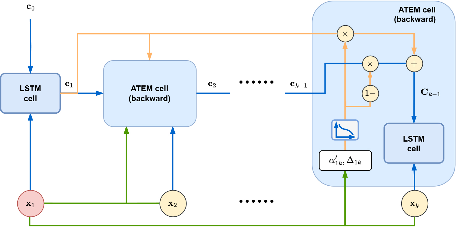$\mathbf{x}_{1}$ is the observation to be detected and $\mathbf{x}_{2},\mathbf{x}_{3},\dots,\mathbf{x}_{k}$ are the historical observations. The update of the hidden states is the same as standard LSTM. The previous cell state $\mathbf{C}_{t-1}^{\prime}$ of the $t$ -th observation is adjusted by weighting and accumulating the first cell state $\mathbf{c}_{1}^{\prime}$ and previous cell state $\mathbf{c}_{t-1}^{\prime}$ . ATEM derives the weights by attention mechanism ( $\alpha^{\prime}$ ) and the time interval ( $\Delta$ ).

Here forward ATEM has an attention mechanism that can collect multiple previous memories. Inspired by ATTAIN [21], in a given sequence $\mathbf{X}_{i}^{k}$ , ATEM have

$\displaystyle e_{tj}=\mathbf{x}_{t}^{\mathsf{T}}\mathbf{W}_{\alpha}\mathbf{x}_% {j},$ (14) $\displaystyle\mathbf{a}_{i}=\mathrm{softmax}(e_{i,i-k+1},e_{i,i-k+2},\dots,e_{% i,i-1}),$ (15) $\displaystyle\mathbf{c}_{i-1}=\Sigma_{j=i-k+1}^{j=i-1}\alpha_{ij}\mathbf{c}_{j% }\cdot g_{c}(\Delta s_{ij}),$ (16)

where $\mathbf{a}_{i}=(\alpha_{i,i-k+1},\alpha_{i,i-k+2},\dots,\alpha_{i,i-1})$ , $\alpha_{ij}$ is attention weight from $j$ -th input to the $i$ -th input, $\mathbf{c}_{j}$ is the cell states output by the standard LSTM, $\Delta s_{ij}=s_{i}-s_{j}$ is the time interval from the $j$ -th observation to the $i$ -th observation. The network is based on the standard LSTM and the $\mathbf{c}_{i-1}$ needed for the last observation in each sequence is calculated by Eq. (16).

Figure 5 illustrates our backward ATEM. In the backward process, the last observation to be detected is input to the standard LSTM first. Its information will be passed as key information in the standard LSTM. The cell state of it will be retained at each time step.

Reversing the sequence $\mathbf{X}$ , ${\mathbf{X}_{i}^{k}}^{\prime}=(\mathbf{x}_{i},\mathbf{x}_{i-1},\dots,\mathbf{x% }_{i-k+1})$ is obtained. For ease of understanding and expression, ${\mathbf{X}_{i}^{k}}^{\prime}$ is renumbered as $(\mathbf{x}_{1},\mathbf{x}_{2},\dots,\mathbf{x}_{k})$ . Note that the timestamp does not change due to renumbering. The backward network is given by

$\displaystyle{\alpha}^{\prime}_{tj}=\sigma(\mathbf{x}_{t}^{\mathsf{T}}\mathbf{% W}^{\prime}_{\alpha}\mathbf{x}_{j}),$ (17) $\displaystyle\mathbf{C}^{\prime}_{t-1}=\alpha^{\prime}_{1t}g_{c}(\Delta s_{tj}% )\mathbf{c}^{\prime}_{1}+(1-\alpha^{\prime}_{1t}g_{c}(\Delta s_{tj}))\mathbf{c% }^{\prime}_{t-1},$ (18)

where $\mathbf{c}^{\prime}_{t-1}$ is the cell state of the backward ATEM output at the time step $t-1$ , $2\leqslant t\leqslant i$ . Then, $\mathbf{c}_{t-1}$ of the standard LSTM in Eq. (4) is replaced with $\mathbf{C}^{\prime}_{t-1}$ for generating new cell state.

Now we discuss how to make use of the results of forward ATEM depicted in Fig. 4 with backward ATEM depicted in Fig. 5. The last hidden states of the forward ATEM and backward ATEM are fed into a Multi-Layer Perception (MLP) to predict the probability that the last observation in the sequence is anomalous data, i.e., ${p}_{i}$ . The binary prediction is then given by

$\displaystyle\hat{y}_{i}=\left\{\begin{array}[]{ll}0,&\textrm{ if }p_{i}<\eta;% \\ 1,&\textrm{ otherwise},\\ \end{array}\right.$ (19)

where $0\leqslant\eta\leqslant 1$ is a threshold. Due to the sparse number of positive classes, the $F_{1}$ -score will be used to evaluate the effectiveness of the model. Instead of setting $\eta=0.5$ directly, ATIN calculates the peak $F_{1}$ -score by setting the optimal $\eta$ value.

The number of samples in the positive and negative classes is unbalanced (positive: negative $\approx 1:5$ ). To prevent a large number of simple negative class from overwhelming the model during training, a specific prediction loss function is employed. The loss function is as follows:

$\displaystyle\mathcal{L}_{p}(y_{i},p_{i})=\mathrm{FL}(y_{i},p_{i},\gamma,\beta),$ (20)

where FL means the function of Focal Loss [44], $\gamma$ is the weight factor and $\beta$ is the focusing parameter. Both $\gamma$ and $\beta$ are hyperparameters.

3.3 Time-aware decay function

The range of time intervals can vary and may be very short minutes, seconds, or longer days. Several works propose different decay functions [45, 19]. In our task, the time interval between each observation is days. According to the guidelines of these works, the decay function for the cell state [19] in Eqs (7), (16) and (17) is

$\displaystyle g_{c}(\Delta)=1/\log(\mathrm{e}+\Delta),$ (21)

and the decay function for the hidden states [20] in Eq. (11) is

$\displaystyle g_{h}(\Delta)=\exp(-\Delta).$ (22)

[b] : ATIN

[1] Original data matrix $\mathbf{X}_{i}^{k}$ , masking matrix $\mathbf{M}_{i}^{k}$ , timestamps matrix $\mathbf{T}_{i}^{k}$ , label $y_{i}$ Probability positive $p_{i}$ $\hat{\mathbf{X}_{i}^{k}},\hat{\mathbf{X}_{i}^{k}}^{\prime},\mathbf{h}_{i}^{k},% {\mathbf{h}_{i}^{k}}^{\prime}=\text{TI-LSTM}(\mathbf{X}_{i}^{k},\mathbf{M}_{i}% ^{k},\mathbf{T}_{i}^{k})$ ; // Imputation and extraction of sequence features. See Section 3.1. $\mathbf{Z}_{i}^{k}={\mathbf{h}_{i}^{k}\circ{\mathbf{h}_{i}^{k}}^{\prime}\circ{% \mathbf{X}}_{i}^{k}}$ ; // Concatenate extracted and original features. $\mathbf{h}_{i},\mathbf{h}_{i-k+1}^{\prime}=\text{ATEM}(\mathbf{Z}_{i}^{k},% \mathbf{T}_{i}^{k})$ ; // Accumulation of historical information. See Section 3.2. $p_{i}=\text{MLP}(\mathbf{h}_{i}\circ\mathbf{h}^{\prime}_{i-k+1})$ ; // Calculate the probability that the instance is positive. $\mathcal{L}={\lambda_{e}}\mathcal{L}_{e}(\mathbf{X}_{i}^{k},\hat{\mathbf{X}_{i% }^{k}},\mathbf{M}_{i}^{k},q)+{\lambda_{c}}\mathcal{L}_{c}(\hat{\mathbf{X}}_{i}% ^{k},{\hat{\mathbf{X}_{i}^{k}}^{\prime},q})+{\lambda_{p}}\mathcal{L}_{p}(y_{i}% ,p_{i})$ ; // Update the model parameters with a weighted sum of losses. See Section 3.1 for $\mathcal{L}_{e}$ and $\mathcal{L}_{c}$ . See Section 3.2 for $\mathcal{L}_{p}$ .

3.4 Anomalous production data detection with ATIN

The overview of ATIN is presented in Fig. 2. Algorithm 3.3 summarizes the forward process of ATIN. TI-LSTM and ATEM form a network structure like stacked RNN. TI-LSTM performs preliminary computation of hidden states $\mathbf{h}_{i}^{k}$ , ${\mathbf{h}_{i}^{k}}^{\prime}$ and estimations $\hat{\mathbf{X}_{i}^{k}}$ , $\hat{\mathbf{X}_{i}^{k}}^{\prime}$ . It learns sequence features based on the observed data and tries to fill in the missing values. The hidden states contain the features of the given sequence at each time stamp. TI-LSTM is not for the downstream task of anomaly detection but for the task of extracting sequence features and imputation (estimation). ATEM is used to address anomaly detection. It takes the concatenation of the extracted feature sequences ( $\mathbf{h}_{i}^{k},{\mathbf{h}_{i}^{k}}^{\prime}$ ) and the original sequences ${\mathbf{X}}_{i}^{k}$ as input and the forward and backward networks derive their final hidden states $\mathbf{h}_{i}$ and $\mathbf{h}_{i-k+1}^{\prime}$ , respectively. Then the probability $p_{i}$ that the last observation is a positive class will be calculated by MLP. The binary prediction is calculated according to Eq. (19). Ultimately, the estimation loss, consistency loss, and prediction loss are assigned weights and summed. Subsequently, backpropagation utilizes this total loss to update the model parameters.

4. Experiments

This section reports experimental results on a real production well dataset. The software and hardware environments are Pytorch and an NVIDIA GeForce RTX 3060 laptop.

4.1 Dataset

Our dataset includes production data from 35 production wells in an oil field in Iraq. Each producing well is characterized by multivariate time series with 26 features. Production data is collected from June 21, 2011, to March 14, 2022. Features are well type, nozzle size, pump frequency, fluid rate, water cut, wellhead pressure, casing pressure, back pressure, and a total of 26 features. The record of each day has a remark. Based on these remarks, only the records that have measured behaviors are extracted to prepare datasets with different sequence lengths. In total, 18,764 sequences of length $k=16$ are included in the collated dataset. The time span of each sequence is at least 16 days, with an average span of 55 days. All sequences are arranged in chronological order and divided into three sets: the first 70% is the training set, and the remaining 30% is used as the test set. The training set contains 17.61% positive class sequences, while the test set contains 22.45% positive class sequences. The percentage of abnormal data varies in different time periods. Table 2 provides detailed information on the datasets used in our study, including the sequence length, the minimum and average time span corresponding to the sequence length, as well as the proportion of positive class in the training and test sets.

Table 2
Datasets

Num of sequences	Sequence length	Time span (days)		Positive rate (%)
		Min	Avg	Training set	Test set
18764	16	16	55	17.61	22.45
17680	32	35	109	17.57	21.65
17344	48	56	163	17.60	21.45

4.2 Experimental setting

Experimental protocol: ATIN is trained by an Adam optimizer with learning rate 0.001 and batch size 32. The training epochs is 50, and the number of hidden units for RNNs is 16. The loss weights were manually established as $\lambda_{e}=1$ , $\lambda_{c}=5$ , and $\lambda_{p}=5$ , ensuring that the individual losses maintain a comparable order of magnitude. We normalize the values for all tasks to zero as the mean and unit variance to achieve stable training.

Evaluation metrics: The performance of the model is assessed by the peak $F_{1}$ [46], AUC, and the balanced F Score of the $F_{1}$ -score and accuracy abbreviated as FA-score. The basis of $F_{1}$ include

$\displaystyle\text{Accuracy}=\frac{\text{TP}+\text{TN}}{\text{TP}+\text{TN}+% \text{FP}+\text{FN}},$ (23) $\displaystyle\text{Precision}=\frac{\text{TP}}{\text{TP}+\text{FP}},$ (24) $\displaystyle\text{Recall}=\frac{\text{TP}}{\text{TP}+\text{FN}},$ (25)

where TP is True Positive, TN is True Negative, FP is False Positive and FN is False Negative. Precision quantifies the proportion of correctly identified positive predictions among all instances classified as positive. Recall, also known as sensitivity, indicates the model’s effectiveness in detecting existing anomalies within the dataset.

$F_{1}$ depicts the overall prediction performance based on the balance between precision and recall. It is given by

$\displaystyle F_{1}\text{-score}=\frac{2*\text{Precision}*\text{Recall}}{\text% {Precision}+\text{Recall}}.$ (26)

FA-score is used to select the final appropriate threshold. It is given by

$\displaystyle\text{FA-score}=\frac{2*F_{1}*\text{Accuracy}}{F_{1}+\text{% Accuracy}}.$ (27)

In Section 4.3, a particular explanation will be provided for utilizing the FA-score. The $F_{1}$ -score and Accuracy corresponding to the FA-score are also evaluation metrics, i.e., $F_{1}$ -score (FA) and Acc (FA).

The receiver operating characteristic (ROC) curve is a graphical representation illustrating the relationship between the true positive rate (y-axis) and the false positive rate (x-axis) across various decision thresholds. AUC, which stands for Area Under the Curve, quantifies the extent of the region beneath the ROC curve. For reference, a naive classifier corresponds to an AUC value of 0.5, indicating random performance. On the other hand, a perfect classifier achieves an AUC value of 1.0.

The computation of peak $F_{1}$ resembles that of ROC curve. $F_{1}$ -scores are computed across different classification thresholds, and the highest $F_{1}$ -score is identified as the peak $F_{1}$ . It is used to evaluate the upper limit of performance for each model.

Models: Each algorithm is randomly initialized with parameters, and each experiment is repeated 18 times. For all models, the hidden state of the last observation is input to the same MLP with two hidden layers for Deriving $p_{i}$ . The loss functions are all Focal Loss, with weight factor $\gamma=0.75$ , focusing parameter $\beta=2$ .

Our baseline methods are the following.

•

LSTM [15]: Stacked standard LSTM with 2 layers. All of our work is built upon the classical time series model.

•

mTAN [27]:1

https://github.com/reml-lab/mTAN.git.

Using Multi-Time Attention Mechanism that takes irregularly sampled time points and the corresponding values as keys and values. It allows flexible imputation of missing values.

•

GRU-D [18]: The missing is filled based on the last observation and global mean. A decay mechanism that is trainable is utilized by it.

•

BRITS [20]:2

https://github.com/caow13/BRITS.git.

Bidirectional RNN network that combines the correlation between individual features and BRIT-I for missing filling. The multi-task learning approach employed in it facilitates better feature learning from the sequences.

•

T-LSTM [19]:3

https://github.com/illidanlab/T-LSTM.git.

The short-term memory component of the cell state decays according to irregular sampling intervals. This method addresses the challenge of handling continuous missing observations.

•

ATTAIN [21]: Using the global attention mechanism, all historical cell states are accumulated as new cell state input for the current observation. It addresses the issue of gradient vanishing commonly encountered in RNNs and employs a time decay function to modulate the flow of information.

Ablation experiments are also performed to show the performance gains achieved by our Time-Aware Mechanism and ATEM:

•

I-ATTAIN: BRIT-I for the first layer to process the sequence of inputs, ATTAIN for the second layer to Detect anomalies.

•

TI-ATTAIN: TI-LSTM for the first layer to process the sequence of the inputs, and ATTAIN as the abnormal detection layer.

•

I-ATEM: BRIT-I for the first layer to process the sequence of the inputs, and ATEM as the abnormal detection layer.

•

FTI-ATTAIN: Forward TI-LSTM without consistency loss works for processing the sequence of the inputs.

To validate the reliability of time perception, a comparative analysis is conducted between I-ATTAIN and TI-ATTAIN, as well as between I-ATEM and ATIN. The objective is to assess the effectiveness and accuracy of these respective models in capturing temporal information. The performance evaluation of I-ATTAIN against I-ATEM and TI-ATTAIN against ATIN provides critical insights into the robustness and viability of ATEM, the anomaly detection framework under investigation. FTI-ATTAIN is employed to validate the efficacy of forward and backward networks.

4.3 Results

Experiments are conducted using datasets with sequence lengths of 16, 32, and 48, respectively. Table 3 shows scores of each baseline model and ATIN. The effectiveness of mTAN improves as the sequence grows. mTAN has good imputation and classification for data with correlation with time stamps. But it does not work well in anomalous production data detection. This shows that Multi-Time Attention Mechanism is inapplicable to production data anomaly detection. The non-time embedded model has better results. ATTAIN has the best performance in the baseline methods. This is due to its Temporal Convolutional Network-like structure and a special attention mechanism. GRU-D implicitly models missing values through a feature-level decay mechanism (decaying hidden state) and is better in terms of performance. T-LSTM does not have the same feature-level decay mechanism as GRU-D, but it captures the information of the observation interval. It is worth noting that BRITS is capable of interpolation, but the classification performance is not outstanding. The performance issue of BRITS is also explained in Section 3.2.

Table 3
Performance ( $\pm$ standard deviation) of baselines and our approach

Sequence length	Method	FA-score	$F_{1}$ -score (FA)	Acc (FA)	AUC	Peak $F_{1}$
16	LSTM	$0.5370_{\pm 0.0143}$	$0.4334_{\pm 0.0139}$	$0.7063_{\pm 0.0266}$	$0.7031_{\pm 0.0135}$	$0.4435_{\pm 0.0110}$
	mTAN	$0.4602_{\pm{0.0128}}$	$0.3761_{\pm{0.0075}}$	$0.5937_{\pm{0.0332}}$	$0.6352_{\pm{0.0027}}$	$0.3934_{\pm{0.0029}}$
	ATTAIN	$0.5711_{\pm{0.0129}}$	$0.4665_{\pm{0.0160}}$	$0.7371_{\pm{0.0202}}$	$0.7374_{\pm{0.0142}}$	$0.4754_{\pm{0.0146}}$
	GRU-D	$0.5666_{\pm{0.0225}}$	$0.4599_{\pm{0.0210}}$	$0.7381_{\pm{0.0261}}$	$0.7233_{\pm{0.0199}}$	$0.4697_{\pm{0.0206}}$
	BRITS	$0.5523_{\pm{0.0278}}$	$0.4453_{\pm{0.0269}}$	$0.7272_{\pm{0.0272}}$	$0.7072_{\pm{0.0271}}$	$0.4525_{\pm{0.0258}}$
	T-LSTM	$0.5393_{\pm{0.0182}}$	$0.4392_{\pm{0.0158}}$	$0.6991_{\pm{0.0316}}$	$0.7043_{\pm{0.0201}}$	$0.4488_{\pm{0.0172}}$
	ATIN	$\textbf{0.5982}_{\pm{0.0163}}$	$\textbf{0.4936}_{\pm{0.0118}}$	$\textbf{0.7786}_{\pm{0.0115}}$	$\textbf{0.7577}_{\pm{0.0107}}$	$\textbf{0.4972}_{\pm{0.0136}}$
32	LSTM	$0.5332_{\pm 0.0193}$	$0.4291_{\pm 0.0158}$	$0.7053_{\pm 0.0382}$	$0.6982_{\pm 0.0184}$	$0.4401_{\pm 0.0125}$
	mTAN	$0.4773_{\pm{0.0153}}$	$0.3874_{\pm{0.0074}}$	$0.6240_{\pm{0.0510}}$	$0.6353_{\pm{0.0043}}$	$0.4005_{\pm{0.0031}}$
	ATTAIN	$0.5820_{\pm{0.0193}}$	$0.4792_{\pm{0.0191}}$	$0.7439_{\pm{0.0270}}$	$0.7418_{\pm{0.0176}}$	$0.4836_{\pm{0.0177}}$
	GRU-D	$0.5654_{\pm{0.0207}}$	$0.4622_{\pm{0.0207}}$	$0.7285_{\pm{0.0213}}$	$0.7196_{\pm{0.0235}}$	$0.4690_{\pm{0.0185}}$
	BRITS	$0.5376_{\pm{0.0141}}$	$0.4288_{\pm{0.0130}}$	$0.7211_{\pm{0.0232}}$	$0.6856_{\pm{0.0176}}$	$0.4356_{\pm{0.0141}}$
	T-LSTM	$0.5434_{\pm{0.0151}}$	$0.4424_{\pm{0.0150}}$	$0.7049_{\pm{0.0274}}$	$0.6989_{\pm{0.0142}}$	$0.4511_{\pm{0.0128}}$
	ATIN	$\textbf{0.6029}_{\pm{0.0115}}$	$\textbf{0.4996}_{\pm{0.0124}}$	$\textbf{0.7603}_{\pm{0.0176}}$	$\textbf{0.7579}_{\pm{0.0114}}$	$\textbf{0.5033}_{\pm{0.0124}}$
48	LSTM	$0.5395_{\pm 0.0236}$	$0.4382_{\pm 0.0298}$	$0.7022_{\pm 0.0221}$	$0.6937_{\pm 0.0227}$	$0.4478_{\pm 0.0175}$
	mTAN	$0.4915_{\pm{0.0056}}$	$0.3948_{\pm{0.0092}}$	$0.6518_{\pm{0.0212}}$	$0.6288_{\pm{0.0037}}$	$0.4059_{\pm{0.0054}}$
	ATTAIN	$0.5853_{\pm{0.0184}}$	$0.4779_{\pm{0.0188}}$	$0.7556_{\pm{0.0243}}$	$0.7411_{\pm{0.0183}}$	$0.4863_{\pm{0.0183}}$
	GRU-D	$0.5694_{\pm{0.0273}}$	$0.4682_{\pm{0.0259}}$	$0.7271_{\pm{0.0335}}$	$0.7191_{\pm{0.0289}}$	$0.4763_{\pm{0.0239}}$
	BRITS	$0.5406_{\pm{0.0197}}$	$0.4321_{\pm{0.0201}}$	$0.7226_{\pm{0.0248}}$	$0.6824_{\pm{0.0213}}$	$0.4406_{\pm{0.0179}}$
	T-LSTM	$0.5463_{\pm{0.0190}}$	$0.4489_{\pm{0.0224}}$	$0.6987_{\pm{0.0171}}$	$0.6990_{\pm{0.0181}}$	$0.4571_{\pm{0.0184}}$
	ATIN	$\textbf{0.5983}_{\pm{0.0120}}$	$\textbf{0.4921}_{\pm{0.0159}}$	$\textbf{0.7636}_{\pm{0.0140}}$	$\textbf{0.7500}_{\pm{0.0101}}$	$\textbf{0.4979}_{\pm{0.0132}}$

Table 4

Ablation study

Sequence length	Method	FA-score	$F_{1}$ -score (FA)	Acc (FA)	AUC	Peak $F_{1}$
16	I-ATTAIN	$0.5926_{\pm{0.0125}}$	$0.4859_{\pm{0.0145}}$	$0.7596_{\pm{0.0151}}$	$0.7514_{\pm{0.0112}}$	$0.4928_{\pm{0.0146}}$
	TI-ATTAIN	$0.5962_{\pm{0.0117}}$	$0.4895_{\pm{0.0130}}$	$0.7627_{\pm{0.0181}}$	$0.7548_{\pm{0.0107}}$	$0.4951_{\pm{0.0124}}$
	I-ATEM	$0.5958_{\pm{0.0156}}$	$0.4871_{\pm{0.0145}}$	$0.7672_{\pm{0.0159}}$	$0.7530_{\pm{0.0137}}$	$0.4917_{\pm{0.0146}}$
	FTI-ATTAIN	${0.5899_{\pm{0.0120}}}$	${0.4834_{\pm{0.0153}}}$	${0.7601_{\pm{0.0142}}}$	${0.7494_{\pm{0.0144}}}$	${0.4874_{\pm{0.0132}}}$
	ATIN	$\textbf{0.5982}_{\pm{0.0163}}$	$\textbf{0.4936}_{\pm{0.0118}}$	$\textbf{0.7786}_{\pm{0.0115}}$	$\textbf{0.7577}_{\pm{0.0107}}$	$\textbf{0.4972}_{\pm{0.0136}}$
32	I-ATTAIN	$0.5960_{\pm{0.0137}}$	$0.4908_{\pm{0.0161}}$	$0.7591_{\pm{0.0154}}$	$0.7501_{\pm{0.0100}}$	$0.4950_{\pm{0.0134}}$
	TI-ATTAIN	$0.6000_{\pm{0.0136}}$	$0.4933_{\pm{0.0167}}$	$\textbf{0.7661}_{\pm{0.0106}}$	$0.7511_{\pm{0.0110}}$	$0.4983_{\pm{0.0150}}$
	I-ATEM	$0.5985_{\pm{0.0103}}$	$0.4944_{\pm{0.0138}}$	$0.7580_{\pm{0.0187}}$	$0.7506_{\pm{0.0139}}$	$0.4970_{\pm{0.0183}}$
	FTI-ATTAIN	${0.5953_{\pm{0.0133}}}$	${0.4887_{\pm{0.0150}}}$	${0.7584_{\pm{0.0171}}}$	${0.7496_{\pm{0.0159}}}$	${0.4901_{\pm{0.0128}}}$
	ATIN	$\textbf{0.6029}_{\pm{0.0115}}$	$\textbf{0.4996}_{\pm{0.0124}}$	$0.7603_{\pm{0.0176}}$	$\textbf{0.7579}_{\pm{0.0114}}$	$\textbf{0.5033}_{\pm{0.0124}}$
48	I-ATTAIN	$0.5974_{\pm{0.0118}}$	$0.4920_{\pm{0.0151}}$	$0.7608_{\pm{0.0119}}$	$0.7469_{\pm{0.0118}}$	$0.4960_{\pm{0.0143}}$
	TI-ATTAIN	$0.5936_{\pm{0.0123}}$	$0.4892_{\pm{0.0141}}$	$0.7549_{\pm{0.0149}}$	$0.7459_{\pm{0.0101}}$	$0.4942_{\pm{0.0124}}$
	I-ATEM	$0.5982_{\pm{0.0116}}$	$\textbf{0.4925}_{\pm{0.0135}}$	$0.7622_{\pm{0.0157}}$	$0.7492_{\pm{0.0130}}$	$\textbf{0.4983}_{\pm{0.0123}}$
	FTI-ATTAIN	${0.5888_{\pm{0.0125}}}$	${0.4865_{\pm{0.0149}}}$	${0.7563_{\pm{0.0159}}}$	${0.7413_{\pm{0.0155}}}$	${0.4903_{\pm{0.0124}}}$
	ATIN	$\textbf{0.5983}_{\pm{0.0120}}$	$0.4921_{\pm{0.0159}}$	$\textbf{0.7636}_{\pm{0.0140}}$	$\textbf{0.7500}_{\pm{0.0101}}$	$0.4979_{\pm{0.0132}}$

Figure 6.

Score curves. Subplots display the score curves of each baseline method and the proposed ATIN. The green curve is the ROC curve. $F_{1}$ -score and accuracy corresponding to each threshold are also shown. The $F_{1}$ -score is depicted in red, and the blue curve represents accuracy.

In Table 4, the ablation experiments verify that the Time-Aware Mechanism and ATEM are effective. TI-ATTAIN outperforms I-ATTAIN for sequence lengths of 16 and 32, which shows that the time-aware mechanism has a gain effect. The same is true for I-ATEM and ATIN. However, the advantage of Time-Aware is not obvious when the sequence length is 48. From the perspectives of TI-ATTAIN and ATIN (as well as I-ATTAIN and I-ATEM), it becomes evident that ATEM exhibits improvements across metrics of FA-score, AUC, and peak $F_{1}$ compared to ATTAIN. FTI-ATTAIN exclusively focuses on forward networks, resulting in a slightly diminished level of effectiveness compared to approaches that consider both forward and backward information.

Figure 6 shows the score curves of each baseline method in the test set. If the binary classification threshold corresponding to peak $F_{1}$ is used, it may sometimes lead to a significant decrease in accuracy. This situation occurs for every method. So FA-score is additionally used to search the appropriate threshold.

Since there may be continuous inconsistencies between the measured data and the expert judgment, the expert tends to trust the measured data at this time. Therefore, the model can be enhanced by using historical labels as input. The effect after adding historical labels as input for each model is shown in Appendix A.

Diverse irregular time series tasks may require the utilization of distinct decay functions. Additionally, cell states and hidden states could also demand diverse decay functions. The experimental exploration of several decay functions is detailed in Appendix B.

5. Conclusions and further works

In this paper, ATIN is proposed for oil production data anomaly detection. This hypothesis-free network not only supports time-aware and imputation but also has a network structure specialized for anomaly data detection. To the best of our knowledge, the proposed ATIN is the first deep learning method for modeling irregular multivariate production time series in oil fields. TI-LSTM models irregular sampling as well as incomplete measurements simultaneously to take advantage of the information that is missing. ATEM has a backward network whose information accumulation improves anomaly detection for new measurements. Experiment results show that ATIN demonstrates more accurate results for anomalous production data detection than state-of-the-art methods.

To further improve the detection, there are still some topics that deserve further investigation.

Transfer learning. This work only trains the model for a general overview of producing wells in an oil field, but each well may have very different production conditions. Transfer learning can be performed on each well individually using the pre-trained ATIN.

Graph neural networks. In a field, producing wells may be drilled into the same reservoir and they may be communicating. In such cases, graph neural networks can be employed to establish the relationship between these wells. TI-LSTM can be used as an encoder for the IMTS of each producing well.

Sequence-Level attention mechanism. In ATEM, an attention mechanism is used for different observations in a given sequence. Further, external information can be used to aid in the detection process [47]. In the first stage, during the training of ATIN, important sequence samples are encoded and stored in the memory module. In the second stage, the attention mechanism is used to query the stored important sequences and evaluate the sequences to be classified.

Combining injection wells. Oil wells are distinguished into producing wells and injection wells, and the production data of producing wells may be greatly influenced by injection wells in the water cut stage. However, they are not taken into account in this work.

In addition to anomaly detection, how the model interprets production data anomalies can offer valuable insights for manual diagnosis. The attention weights utilized in ATEM aid in identifying timestamps linked to anomalous production data, thereby enhancing the interpretability of the detection results. Recently, analyzing production data in petroleum reservoirs to estimate future production has become popular. TI-LSTM can be applied not only for the complementation of irregular multivariate production data but also for the prediction of future production. In the forecasting phase, its ability to infer all characteristics is limited to inferring only yield characteristics.

Footnotes

Acknowledgments

This work is supported by the Central Government Funds of Guiding Local Scientific and Technological Development (No. 2021ZYD0003) and the National Social Science Foundation of China under Grant (No. 22FZXB092).

Appendix

Detection with historical labels

Figure 7.

Score curves with historical labels. Subplots display the score curves of each baseline method and our proposed ATIN. The green curve is the ROC curve. 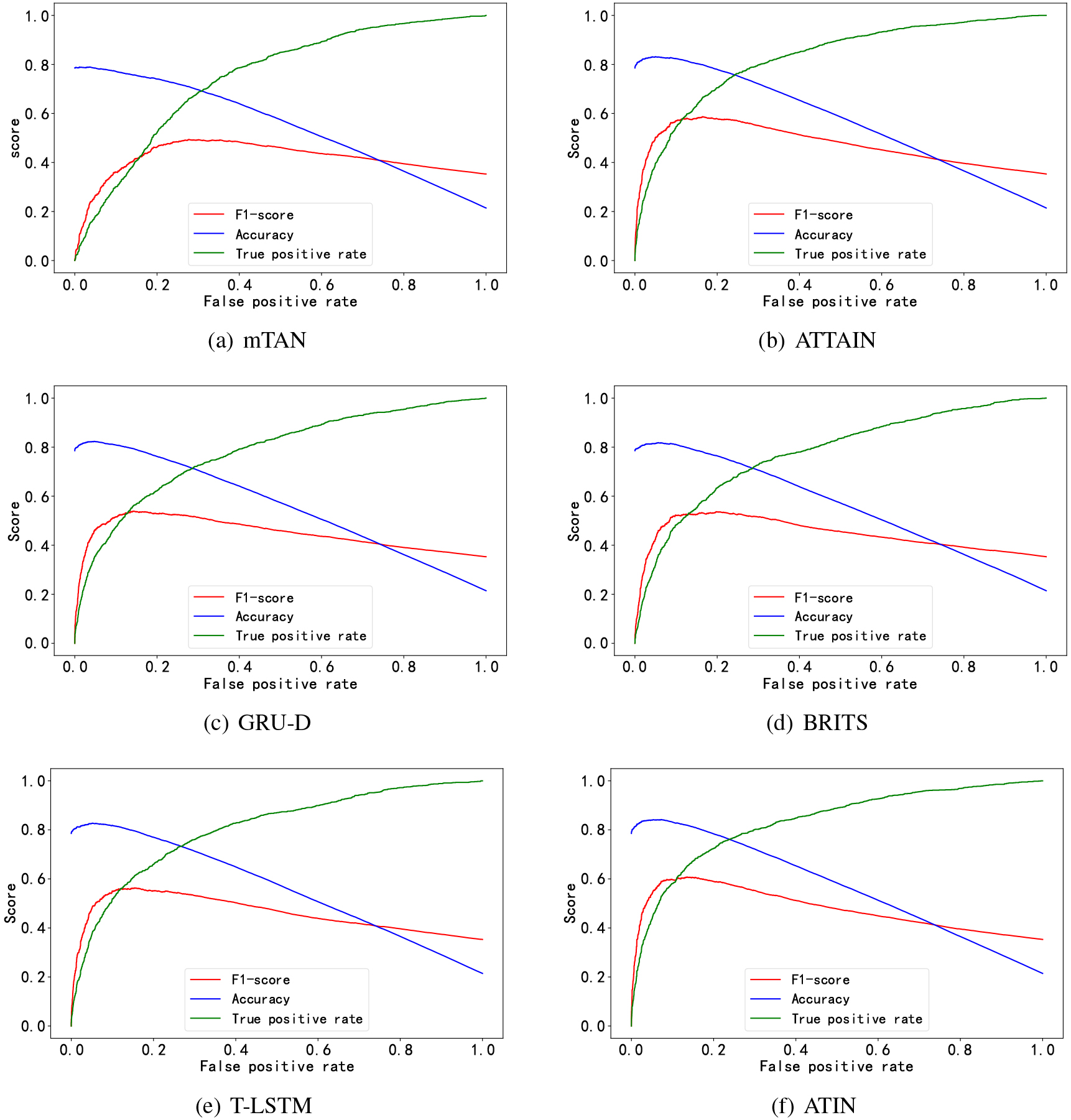$F_{1}$ -score and accuracy corresponding to each threshold are also shown. The $F_{1}$ -score is depicted in red, and the blue curve represents accuracy.

Table 5

Performance with historical labels

Method	FA-score	$F_{1}$ -score (FA)	Acc (FA)	AUC	Peak $F_{1}$
LSTM	$0.6716_{\pm 0.0131}$	$0.5713_{\pm 0.0160}$	$0.8150_{\pm 0.0092}$	$0.8062_{\pm 0.0145}$	$0.5737_{\pm 0.0156}$
mTAN	$0.5800_{\pm 0.0086}$	$0.4864_{\pm 0.0105}$	$0.7183_{\pm 0.0081}$	$0.7399_{\pm 0.0094}$	$0.4894_{\pm 0.0094}$
ATTAIN	$0.6872_{\pm 0.0073}$	$0.5925_{\pm 0.0090}$	$0.8179_{\pm 0.0092}$	$0.8257_{\pm 0.0054}$	$0.5949_{\pm 0.0080}$
GRU-D	$0.6439_{\pm 0.0215}$	$0.5397_{\pm 0.0245}$	$0.7984_{\pm 0.0139}$	$0.7796_{\pm 0.0238}$	$0.5422_{\pm 0.0251}$
BRITS	$0.6288_{\pm 0.0219}$	$0.5248_{\pm 0.0263}$	$0.7850_{\pm 0.0160}$	$0.7777_{\pm 0.0177}$	$0.5300_{\pm 0.0243}$
T-LSTM	$0.6670_{\pm 0.0144}$	$0.5666_{\pm 0.0165}$	$0.8108_{\pm 0.0101}$	$0.8075_{\pm 0.0145}$	$0.5692_{\pm 0.0167}$
ATIN	$\textbf{0.6944}_{\pm 0.0061}$	$\textbf{0.6005}_{\pm 0.0083}$	$\textbf{0.8232}_{\pm 0.0065}$	$\textbf{0.8291}_{\pm 0.0049}$	$\textbf{0.6029}_{\pm 0.0070}$

Table 6

Ablation with decay functions

Method	FA-score	$F_{1}$ -score (FA)	Acc (FA)	AUC	Peak $F_{1}$
I-ATTAIN	$0.6905_{\pm 0.0065}$	$0.5926_{\pm 0.0084}$	$\textbf{0.8273}_{\pm 0.0055}$	$0.8255_{\pm 0.0047}$	$0.5963_{\pm 0.0083}$
TI-ATTAIN	$0.6905_{\pm 0.0066}$	$0.5958_{\pm 0.0084}$	$0.8212_{\pm 0.0071}$	$0.8263_{\pm 0.0055}$	$0.5979_{\pm 0.0076}$
I-ATEM	$0.6922_{\pm 0.0067}$	$0.5976_{\pm 0.0082}$	$0.8223_{\pm 0.0061}$	$0.8285_{\pm 0.0045}$	$0.5974_{\pm 0.0076}$
FTI-ATTAIN	${0.6901_{\pm{0.0069}}}$	${0.5935_{\pm{0.0082}}}$	${0.8223_{\pm{0.0068}}}$	${0.8243_{\pm{0.0044}}}$	${0.5953_{\pm{0.0072}}}$
ATIN	$\textbf{0.6944}_{\pm 0.0061}$	$\textbf{0.6005}_{\pm 0.0083}$	$0.8232_{\pm 0.0065}$	$\textbf{0.8291}_{\pm 0.0049}$	$\textbf{0.6029}_{\pm 0.0070}$

Based on expert experience, experts will believe the current measurement if there are recent consecutive historical measurements that are judged to be anomalous. In brief, the historical labels will influence the current anomaly detection. Therefore, we incorporate historical labels into the inputs of the model. Equation (10) is adjusted as

(28) $\displaystyle\mathbf{x}_{t}^{c}=((\mathbf{m}_{t}\odot\mathbf{x}_{t})+(1-% \mathbf{m}_{t})\odot\hat{\mathbf{x}}_{t})\circ\mathbf{y}_{t}.$

To maintain the format of the input data, at the last point, we let $\mathbf{y}_{i}=0$ .

Table 5 shows the effect with the addition of historical labels when the sequence length is 16. The results of all models are significantly improved. The proposed ATIN still achieves outstanding performance. Meanwhile, ATTAIN and the proposed model with an attention mechanism (I-ATTAIN, TI-ATTAIN, I-ATEM, ATIN) performed more consistently in all evaluation metrics. Interestingly, LSTM outperforms other baseline models as it is aided by historical labels to make a better classification. In contrast, models such as mTAN, BRITS, T-LSTM, and GRU-D, which are specifically designed for IMTS, fail to make optimal use of historical labels. Table 6 shows the results of the ablation experiments. Time-Aware and ATEM continue to have gaining effects. Figure 7 shows the score curves of each respective model after adding the historical labels.

Detection with different decay functions

For different tasks, their best-dapted decay functions may be varied. Here are a few of the most commonly used decay functions:

(29) $\displaystyle g_{\exp}(\Delta)=\exp(-\Delta),$ (30) $\displaystyle g_{\log}(\Delta)=1/\log(\mathrm{e}+\Delta),$ (31) $\displaystyle g_{\textit{rcp}}(\Delta)=1/(\Delta+1).$

Using ATIN as the base model, the functions $g_{h}$ and $g_{c}$ are modified separately. The set of sequences with a length of 16 is selected for validation. The row directions in Tables 7–9 are the decay functions for $g_{h}$ and the columns are the decay functions for $g_{c}$ . These tables show the results of different decay functions on the three metrics FA-score, AUC, and peak $F_{1}$ , respectively.

The outcomes demonstrate that employing $g_{\exp}$ for both $g_{c}$ and $g_{h}$ yields superior results in terms of FA-score and peak $F_{1}$ metrics. Regarding the AUC metrics, adopting $g_{\textit{rcp}}$ as the decay function for cell states and $g_{\exp}$ as the decay function for the hidden states improved outcomes.

Table 7

Results (FA-score) with decay functions

$g_{c}$ $g_{h}$	$g_{\exp}$	$g_{\log}$	$g_{\textit{rcp}}$
$g_{\exp}$	$\textbf{0.6002}_{\pm 0.0131}$	$0.5947_{\pm 0.0127}$	$0.5990_{\pm 0.0137}$
$g_{\log}$	$0.5982_{\pm 0.0163}$	$0.5976_{\pm 0.0128}$	$0.5976_{\pm 0.0133}$
$g_{\textit{rcp}}$	$0.5984_{\pm 0.0111}$	$0.5958_{\pm 0.0135}$	$0.5985_{\pm 0.0129}$

Table 8

Results (AUC) with decay functions

$g_{c}$ $g_{h}$	$g_{\exp}$	$g_{\log}$	$g_{\textit{rcp}}$
$g_{\exp}$	$0.7587_{\pm 0.0113}$	$0.7548_{\pm 0.0131}$	$0.7563_{\pm 0.0116}$
$g_{\log}$	$0.7577_{\pm 0.0107}$	$0.7572_{\pm 0.0094}$	$0.7577_{\pm 0.0126}$
$g_{\textit{rcp}}$	$\textbf{0.7593}_{\pm 0.0098}$	$0.7575_{\pm 0.0112}$	$0.7579_{\pm 0.0096}$

Table 9

Results (Peak $F_{1}$ ) with decay functions

$g_{c}$ $g_{h}$	$g_{\exp}$	$g_{\log}$	$g_{\textit{rcp}}$
$g_{\exp}$	$\textbf{0.5007}_{\pm 0.0118}$	$0.4933_{\pm 0.0109}$	$0.4970_{\pm 0.0135}$
$g_{\log}$	$0.4972_{\pm 0.0136}$	$0.4965_{\pm 0.0118}$	$0.4961_{\pm 0.0137}$
$g_{\textit{rcp}}$	$0.4977_{\pm 0.0123}$	$0.4944_{\pm 0.0135}$	$0.4982_{\pm 0.0135}$

In addition, the decay function can be selected based on the validation set. The percentage of training set, validation set, and test machine can be set as desired. For example, in this task, all sequences are arranged chronologically and divided into three groups: the first 70% is the training set, the middle 15% is the validation set, and the remaining 15% is the test set. After training using different decay funtions, the model that performs best on the validation set is selected for the final evaluation. Assuming the validation set and test set share the same data distribution, the experimental outcomes observed on the validation set are expected to closely approximate the experimental outcomes on the test set during the final evaluation.

References

Otchere

D.A.

Ganat

T.O.A.

Gholami

Ridha

, Application of supervised machine learning paradigms in the prediction of petroleum reservoir properties: Comparative analysis of ANN and SVM models, Journal of Petroleum Science and Engineering 200 (2021), 108–182.

Alkinani

H.H.

Al-Hameedi

A.T.

Dunn-Norman

Flori

R.E.

Alsaba

M.T.

Amer

A.S.

, Applications of Artificial Neural Networks in the Petroleum Industry: A Review, in: SPE, 2019, pp. 1–12.

Khan

Louis

, An Artificial Intelligence Neural Networks Driven Approach to Frecast Production in Unconventional Reservoirs – Comparative Analysis with Decline Curve, in: IPTC, 2021, pp. 1–10.

Peng

Rao

Zhao

Zhong

Zhan

Huang

, A proxy model to predict reservoir dynamic pressure profile of fracture network based on deep convolutional generative adversarial networks (DCGAN), Journal of Petroleum Science and Engineering 208 (2022), 109577.

Zeng

Dong

Huang

Liu

Ostadhassan

Bao

, Lithology identification using graph neural network in continental shale oil reservoirs: A case study in Mahu Sag, Junggar Basin, Western China, Marine and Petroleum Geology 150 (2023), 106168.

Min

Wang

Pan

Song

, Fast convex set projection with deep prior for seismic interpolation, Expert Systems with Applications 213 (2023), 119256.

Machado de Almeida Duque

M.C.

Souza Chaves

de Oliveira Monteiro

Velasco Medani

Ferreira Filho

José

, Machine Learning Models To Automatically Validate Petroleum ProductionTests, in: SPE Latin American and Caribbean Petroleum Engineering Conference, 2020, pp. 1–15.

Chaudhary

N.L.

Lee

W.J.

, Detecting and Removing Outliers in Production Data to Enhance Production Forecasting, in: SPE/IAEE Hydrocarbon Economics and Evaluation Symposium, 2016, pp. 1–21.

Tan

Yang

Liu

A.J.

Yip

T.C.-F.

Wong

G.L.-H.

Yuen

, DATA-GRU: Dual-Attention Time-Aware Gated Recurrent Unit for Irregular Multivariate Time Series, in: AAAI, Vol. 34, 2020, pp. 930–937.

10.

Elmabrouk

Shirif

Mayorga

, Artificial neural network modeling for the prediction of oil production, Petroleum Science and Technology 32(9) (2014), 1123–1130.

11.

Muradkhanli

, Neural networks for prediction of oil production, IFAC-PapersOnLine 51(30) (2018), 415–417.

12.

Mamo

B.N.

Dennis

A.Y.

, Artificial neural network based production forecasting for a hydrocarbon reservoir under water injection, Petroleum Exploration and Development 47(2) (2020), 383–392.

13.

Wang

Shi

DOU

, Production prediction at ultra-high water cut stage via Recurrent Neural Network, Petroleum Exploration and Development 47(5) (2020), 1084–1090.

14.

Bao

Gildin

Huang

Coutinho

E.J.R.

, Data-Driven End-To-End Production Prediction of Oil Reservoirs by EnKF-Enhanced Recurrent Neural Networks, in: SPE, 2020, pp. 1–21.

15.

Hochreiter

Schmidhuber

, Long short-term memory, Neural Computation 9(8) (1997), 1735–1780.

16.

Xiao

Wang

Zhang

, Time-series production forecasting method based on the integration of Bidirectional Gated Recurrent Unit (Bi-GRU) network and Sparrow Search Algorithm (SSA), Journal of Petroleum Science and Engineering 208 (2022), 109309.

17.

Xiao

Wang

Zhang

, Multistep ahead multiphase production prediction of fractured wells using bidirectional gated recurrent unit and multitask learning, SPE 28(01) (2023), 381–400.

18.

Che

Purushotham

Cho

Sontag

Liu

, Recurrent neural networks for multivariate time series with missing values, Scientific Reports 8(1) (2018), 1–12.

19.

Baytas

I.M.

Xiao

Zhang

Wang

Jain

A.K.

Zhou

, Patient Subtyping via Time-Aware LSTM Networks, in: SIGKDD, 2017, pp. 65–74.

20.

Cao

Wang

Zhou

, Brits: Bidirectional Recurrent Imputation for Time Series, in: NeurIPS, Vol. 31, 2018, pp. 1–11.

21.

Zhang

Yang

Ivy

Chi

, ATTAIN: Attention-based Time-Aware LSTM Networks for Disease Progression Modeling, in: IJCAI, 2019, pp. 4369–4375.

22.

Zhang

Thadajarassiri

Sen

Rundensteiner

, Time-Aware Transformer-based Network for Clinical Notes Series Prediction, in: Machine Learning for Healthcare Conference, PMLR, 2020, pp. 566–588.

23.

Ruan

Korpeoglu

Kumar

Achan

, Self-attention with Functional Time Representation Learning, in: NeurIPS, Vol. 1–11, 2019, p. 119619.

24.

Song

Rajan

Thiagarajan

Spanias

, Attend and Diagnose: Clinical Time Series Analysis Using Attention Models, in: AAAI, Vol. 32, 2018, pp. 4091–4098.

25.

Kazemi

S.M.

Goel

Eghbali

Ramanan

Sahota

Thakur

Smyth

Poupart

Brubaker

, Time2vec: Learning a Vector Representation of Time, arXiv preprint arXiv:1907.05321, 2019, 1–16.

26.

Vaswani

Shazeer

Parmar

Uszkoreit

Jones

Gomez

A.N.

Kaiser

Ł.

Polosukhin

, Attention Is All You Need, in: NeurIPS, Vol. 30, 2017, pp. 1–11.

27.

Shukla

S.N.

Marlin

, Multi-Time Attention Networks for Irregularly Sampled Time Series, in: ICLR, 2021, pp. 1–15.

28.

Shukla

S.N.

Marlin

, Heteroscedastic Temporal Variational Autoencoder For Irregularly Sampled Time Series, in: ICLR, 2022, pp. 1–20.

29.

Cai

Gao

Ngiam

K.Y.

Ooi

B.C.

Zhang

Yuan

, Medical Concept Embedding with Time-Aware Attention, in: IJCAI, 2018, pp. 3984–3990.

30.

Chen

R.T.

Rubanova

Bettencourt

Duvenaud

D.K.

, Neural Ordinary Differential Equations, in: NeurIPS, Vol. 31, 2018, pp. 1–13.

31.

De Brouwer

Simm

Arany

Moreau

, GRU-ODE-Bayes: Continuous modeling of sporadically-observed time series, in: NeurIPS, Vol. 32, 2019, pp. 1–12.

32.

Rubanova

Chen

R.T.

Duvenaud

D.K.

, Latent Ordinary Differential Equations for Irregularly-Sampled Time Series, in: NeurIPS, Vol. 32, 2019, pp. 1–11.

33.

Herrera

Krach

Teichmann

, Neural Jump Ordinary Differential Equations: Consistent Continuous-Time Prediction and Filtering, in: ICLR, 2020, pp. 1–10.

34.

Kidger

Morrill

Foster

Lyons

, Neural Controlled Differential Equations for Irregular Time Series, in: NeurIPS, Vol. 33, 2020, pp. 6696–6707.

35.

Morrill

Salvi

Kidger

Foster

, Neural Rough Differential Equations for Long Time Series, in: ICML, PMLR, 2021, pp. 7829–7838.

36.

Hasani

Lechner

Amini

Liebenwein

Ray

Tschaikowski

Teschl

Rus

, Closed-form continuous-time neural networks, Nature Machine Intelligence 4(11) (2022), 992–1003.

37.

Luo

Cai

Zhang

Yuan

, Multivariate Time Series Imputation with Generative Adversarial Networks, in: NeurIPS, Vol. 31, 2018, pp. 1–12.

38.

Miao

Wang

Gao

Mao

Yin

, Generative Semi-supervised Learning for Multivariate Time Series Imputation, in: AAAI, Vol. 35, 2021, pp. 8983–8991.

39.

Kim

Khyalia

, STING: Self-attention based Time-series Imputation Networks using GAN, in: ICDM, 2021, pp. 1264–1269.

40.

Luo

Zhang

Cai

Yuan

, E2GAN: End-to-End Generative Adversarial Networkfor Multivariate Time Series Imputation, in: IJCAI, 2019, pp. 3094–3100.

41.

Zhang

Zhou

Cai

Guo

Ding

Yuan

, Missing value imputation in multivariate time series with end-to-end generative adversarial networks, Information Sciences 551 (2021), 67–82.

42.

Zhang

Ilyas

Rekatsinas

, Attention-Based Learning for Missing Data Imputation in HoloClean, in: MLSys, Vol. 2, 2020, pp. 307–325.

43.

Schirmer

Eltayeb

Lessmann

Rudolph

, Modeling Irregular Time Series with Continuous Recurrent Units, in: ICML, 2022, pp. 19388–19405.

44.

Lin

T.-Y.

Goyal

Girshick

Dollár

, Focal Loss for Dense Object Detection, in: ICCV, 2017, pp. 2980–2988.

45.

Pham

Tran

Phung

Venkatesh

, DeepCare: A Deep Dynamic Memory Model for Predictive Medicine, in: Pacific-Asia Conference on Knowledge Discovery and Data Mining, 2016, pp. 30–41.

46.

Min

Qian

Zhang

Song

Min

, Multi-label active learning through serial–parallel neural networks, Knowledge-Based Systems 251 (2022), 109226.

47.

Tang

Yao

Sun

Aggarwal

Mitra

Wang

, Joint Modeling of Local and Global Temporal Dynamicsfor Multivariate Time Series Forecasting with Missing Values, in: AAAI, Vol. 34, 2020, pp. 5956–5963.

ATIN: Attention-embedded time-aware imputation networks for production data anomaly detection

Abstract

Keywords

1. Introduction

Table 1 Notations

4. Experiments

4.1 Dataset

Table 2 Datasets

Table 3 Performance ( ± standard deviation) of baselines and our approach

Footnotes

Acknowledgments

Appendix

Detection with historical labels

Detection with different decay functions

References

Table 1
Notations

Table 2
Datasets

Table 3
Performance ( $\pm$ standard deviation) of baselines and our approach