Floating-point histograms for exploratory analysis of large scale real-world data sets

Abstract

Histograms are among the most popular methods used in exploratory analysis to summarize univariate distributions. In particular, irregular histograms are good non-parametric density estimators that require very few parameters: the number of bins with their lengths and frequencies. Although many approaches have been proposed in the literature to infer these parameters, most existing histogram methods are difficult to exploit for exploratory analysis in the case of real-world data sets, with scalability issues, truncated data, outliers or heavy-tailed distributions. In this paper, we focus on the G-Enum histogram method, which exploits the Minimum Description Length (MDL) principle to build histograms without any user parameter. We then propose to extend this method by exploiting a new modeling space based on floating-point representation, with the objective of building histograms resistant to outliers or heavy-tailed distributions. We also suggest several heuristics and a methodology suitable for the exploratory analysis of large scale real-world data sets, whose underlying patterns are difficult to recover for digitization reasons. Extensive experiments show the benefits of the approach, evaluated with a dual objective: the accuracy of density estimation in the case of outliers or heavy-tailed distributions, and the effectiveness of the approach for exploratory data analysis.

Keywords

Density estimation histograms model selection minimum description length exploratory analysis

1. Introduction

Histograms are among the most popular methods used in exploratory analysis to summarize univariate distributions. Regular histograms are the simplest savor of histograms to represent a distribution: all bins are of the same width and the only parameter to select is the number of bins. While they are suited to roughly uniform distributions [1], they fail to capture the density of more complex distributions. Irregular histograms are non-parametric piecewise constant density estimators that require very few parameters: the number of bins with their widths and frequencies. Several irregular histogram methods have been proposed in the literature, but they often require user-defined parameters, such as the number of bins or the accuracy $\epsilon$ at which the data is to be approximated. For example, the minimum description length (MDL) histogram methods [1, 2] automatically choose the number of bins and their widths, but these widths need to be a multiples of a user parameter $\epsilon$ . In the context of exploratory analysis, the choice of this parameter is not an easy task, and fully automatic histogram methods are preferable. Several automatic irregular histogram methods have been proposed in the literature, such as the taut string methods based on penalized likelihood [3, 4], the Bayesian blocks histograms based Bayesian regularization [5] or the G-Enum method [6] based on the MDL approach. In a comparison between several regular and irregular histograms methods, the G-Enum method achieves state-of-the-art accuracy for estimated density while being much more scalable than its closest competitors [6]. It is also among the most parsimonious methods, with far fewer intervals than the most accurate alternative methods, which is an essential feature for exploratory analysis when interpretability is an issue. These properties being in line with our main objective in this paper, we focus on this method.

The G-Enum method [6] extends the MDL method [2] with an automatic choice of $\epsilon$ , a fast to compute closed-form evaluation criterion and scalable efficient optimization heuristics. Its modeling space is described on the basis of $\epsilon$ -length elementary bins, where each histogram bin consists of a subset of adjacent $\epsilon$ -length bins. A granularity parameter is exploited to automatically select the $\epsilon$ parameter. Together with efficient linearithmic optimization heuristic, this granulated MDL criterion provides a resilient, efficient and fully automated approach to histogram density estimation. Nevertheless, this method reaches its limits in the case of outliers or heavy-tailed distributions and in the case of real world data sets.

This paper presents an extension of the G-Enum method that exploits the floating-point representation of real number on computers, and a methodology for univariate exploratory analysis of large scale real-world data sets. The first key contributions are related to

histograms for density estimation:

introduction of a space of floating-point bins, as an alternative to equal-width bins,

extension of the G-Enum method with new criterion and algorithm,

extensive experiments in the case of outliers or heavy-tailed distributions.

However, while the method works very well on challenging artificial data sets with known distributions, preliminary experiments show the limitations of the approach when applied to real-world data sets, where the aim is to provide a better understanding of the data through exploratory analysis. The second key contributions are related to

histograms for exploratory analysis:

characterization of some issues that come with real-world data,

proposal of a methodology for effective exploratory analysis using histograms,

illustration with several use cases related to challenging real-world data sets.

The rest of the paper is organized as follows. We briefly recall the G-Enum method in Section 2. We illustrate the limit of histogram methods in the case of outliers and discuss possible solutions to push these limits in Section 3. We introduce the notion of floating-point bins in Section 4, and exploit them to suggest an approach named G-Enum-fp in Section 5. We perform extensive experiments with artificial data sets in Section 6. We then propose a methodology for the exploratory analysis of real-world data sets in Section 7, which we evaluate in Section 8. Finally, we give a summary and suggest future work in Section 9.

2. G-Enum method: Summary

This section is a brief reminder of the G-Enum method [6].

2.1 Problem formulation

We consider a sample of $n$ observations $x^{n}=(x_{1},\ldots,x_{n})$ on the interval $[x_{\min},x_{\max}]$ . Let $\epsilon$ be the approximation accuracy, so that each $x_{j}\in x^{n}$ can be approximated by $\widetilde{x}_{j}\in\mathcal{X}=\{x_{\min}+t\epsilon;t=0,\ldots,E\}$ where $E=L/\epsilon$ and $L=x_{\max}-x_{\min}$ is the ‘domain length’ of the data. We expect to have $E\in\mathbb{N}$ .

Let $\mathcal{C}$ be the set of possible endpoints for sub-intervals as

$\displaystyle\mathcal{C}=\left\{c_{t}=x_{\min}-\frac{\epsilon}{2}+t\epsilon;t=% 0,\ldots,E\right\}.$

These endpoints define $E$ elementary bins of length $\epsilon$ , which are called $\epsilon$ -bins. They are the building blocks of histogram intervals: each combination of $\epsilon$ -bins into $K$ intervals, with $K$ ranging from 1 to $E$ , defines a histogram model. In this range of possibilities, the goal is to select a set of $K-1$ endpoints $C=(c_{1},\ldots,c_{K-1}),c_{k}\in\mathcal{C}$ such that $[c_{0},c_{K}]=[x_{\min}-\epsilon/2,x_{\max}+\epsilon/2]$ is partitioned into $K$ intervals $\{[c_{0},c_{1}],[c_{1},c_{2}],\ldots,[c_{K-1},c_{K}]\}$ that are well-suited to the actual data distribution. Each interval $k$ has a data count of $h_{k}$ entries and a length $L_{k}=c_{k}-c_{k-1}$ , which is a multiple of $\epsilon$ :

$\displaystyle\forall k,\exists E_{k}\in\mathbb{N}\text{ such that }L_{k}=E_{k}\cdot\epsilon$

A histogram model is entirely defined by the choice of the number of intervals, the set of endpoints that define them and their data counts. We thus note a histogram model $\mathcal{M}=(K,C,\{h_{k}\}_{1\leqslant k\leqslant K})$ . The relevance of each model can be measured through different types of MDL criteria, for example using an enumerative criterion.

2.2 Granularity and choice of $\epsilon$

The role of approximation accuracy $\epsilon$ has been studied in [6] for the Enum method, both theoretically and empirically. When $\epsilon$ tends towards 0, or equivalently $E$ tends towards $+\infty$ , the MDL criterion is dominated by the prior terms and the number of intervals decreases asymptotically down to a single interval.

To get rid of this user parameter $\epsilon$ , a new model parameter is introduced, that will automatically be inferred. Let $G$ be the granularity parameter. For a given $E$ , the numerical domain is split into $G$ bins ( $1\leqslant G\leqslant E$ ) of equal width. In practice, the constant $E=10^{9}$ is used, which is both close to the limits of the representation of machine integers and allows to obtain very accurate histograms, with an accuracy of up to one billionth of the value domain. Each of these new elementary bins, that are called $g$ -bins, is composed of $g=E/G$ $\epsilon$ -bins. Each of the intervals of any histogram constructed has then a length that is a multiple of these $g$ -bins. In other words, each interval is no longer composed of a multiple of $\epsilon$ -bins but rather composed of $G_{k}$ $g$ -bins.

This new criterion, which is called G-Enum is still very similar to the MDL-based enumerative criterion Enum for histograms, as shown in Table 1. The resulting method is parameter-free, as it does not depend on any user parameter.1

2.3 Enum and G-Enum criteria for histogram models

Table 1
Term comparison of the Enum and G-Enum criteria

Criterion	Indexing terms	Multinomial terms	Bin index terms
Enum	$\log^{*}K+\log\binom{E+K-1}{K-1}$	$\log\binom{n+K-1}{K-1}+\log\frac{n!}{h_{1}!\ldots h_{K}!}$	$\sum^{K}_{k=1}h_{k}\log E_{k}$
G-Enum	$\log^{}K+\log^{}G+\log{{G+K-1}\choose{K-1}}$	$\log\binom{n+K-1}{K-1}+\log\frac{n!}{h_{1}!\ldots h_{K}!}$	$\sum^{K}_{k=1}h_{k}\log G_{k}+n\log\frac{E}{G}$

Table 1 recalls the Enum criterion for histogram models and its granulated extension G-Enum. The $\log^{*}K$ and $\log^{*}G$ prior terms encode the choice of the number of intervals and of the granularity parameter. They exploit Rissanen’s universal prior for integers [7], that favors small integers, i.e. simpler histograms. The $\log\binom{G+K-1}{K-1}$ term encodes the boundaries of the intervals at the granularity precision. The multinomial terms are used to encode the multinomial distribution of the $n$ instances on the $K$ intervals. They rely on an enumerative criterion with appealing optimality properties [8].The $\sum^{K}_{k=1}h_{k}\log G_{k}+n\log\frac{E}{G}$ term encodes the position of the $h_{k}$ instances of each interval on the $E_{k}=G_{k}\frac{E}{G}$ elementary $\epsilon$ -bins of the interval.

2.4 Optimization algorithms

For additive criteria such as Enum, a dynamic programming algorithm can be applied to obtain the optimal solution. However, its computational complexity is cubic w.r.t. the number endpoints $E$ , making it impractical in the case of large data sets. To achieve a practicable computational complexity, the Enum method exploits a greedy bottom-up optimization heuristic that starts with the most refined histogram based on $\epsilon$ -bins, then merges adjacent intervals until the criterion can no longer be improved. The quality of the model is then improved using post-optimization heuristics, which mainly consist of adding, removing, or moving endpoints around the local optimal solution. Moreover, in the case of the Enum criterion, the optimal endpoints are necessarily close to data points, as demonstrated in [6], which reduces the number of candidate endpoints from $E$ to $O(n)$ , resulting in an overall computational complexity is $O(n\log n$ ) instead of $O(E^{3})$ . Experiments show that the accuracy of histograms optimized using these heuristics is indistinguishable from those using the optimal algorithm, while being much faster to compute. As for the G-Enum method, only the powers of two granularities are considered and the Enum algorithm is called $O(\log E)$ times, the computational complexity remaining $O(n\log n)$ since $E$ is a constant.

2.5 Experimental results

We summarize below the results of the comparative experiments performed to evaluate the G-Enum method [6]. The comparison includes the following irregular and regular histogram methods:

G-Enum, the method summarized in this section,

Enum, the base method, with user parameter $\epsilon=0.01$ ,

NML histograms [2], with user parameter $\epsilon=0.01$ ,

Taut string histograms [3, 9],

RMG histograms [4],

Bayesian blocks[5],

Sturges rule histograms,

Freedman-Diaconis rule histograms [10].

It is worth noting that the Enum and NML methods are similar in that they both require a $\epsilon$ user parameter, share the same modeling space and exploit a MDL approach. They differ in terms of optimized MDL code and computational complexity: Normalized Maximum Likelihood code and $O(E^{3})$ for NML, versus enumerative code and $O(n\log n)$ for Enum. All the other methods are parameter-free.

The histogram methods are evaluated on artificial data sets with known distributions: Normal, Cauchy, Uniform, Triangle, Triangle mixture and Gaussian mixture. The methods are compared on three criteria: accuracy evaluated with the Hellinger distance, parsimony using the number of intervals and computation time. The analysis of the experimental results shows that the G-Enum method achieves state of the art accuracy while being much more parsimonious and faster than its closest competitors.

“Although rarely the best for each distribution type, G-Enum histograms are consistently among the best estimators, and this without the high variability of the other methods. Focusing on irregular histograms, G-Enum is certainly among the most parsimonious in number of intervals. For exploratory analysis, this is an important quality because it makes the interpretation of the results easier and more reliable. G-Enum is also by far the fastest of irregular methods, making it suitable to large data sets.” [6]

In particular, in the case of the heavy-tailed Cauchy distribution with the largest evaluated data set size ( $n=10^{5}$ ) and widest value domain, G-Enum histograms are the most accurate density estimators while being between 10 and 1000 times faster than their accurate competitors.

3. Limits of histogram methods w.r.t. outliers

We first give an illustrative example of the limits of the G-Enum method in the case of outliers, and then discuss possible solutions to push these limits.

3.1 Illustative exemple

Let us consider a data set containing $n=10,000$ data entries distributed according to a Gaussian distribution $G(\mu=0,\sigma=1)$ . The range of the numerical domain is $L=(x_{\max}-x_{\min})$ . As $\sigma=1$ , we have $L\leqslant 10$ with high probability. The range of the numerical domain at $\epsilon$ accuracy is $E=L/\epsilon$ . Let us recall that we have chosen $E=10^{9}$ to be compliant with the computer representation of integers using four bytes. As a matter of fact, computer integers are in the value domain $[-\text{INT\_MAX}$ ; $\text{INT\_MAX}]$ , with $\text{INT\_MAX}=2^{31}\approx 2.10^{9}$ . Using the $E=10^{9}$ precision parameter, the bounds of the histogram intervals are very precise, and the underlying distribution can be very well approximated as the number of data entries $n$ increases.

Let us now assume that we have an outlier data entry in our data set, with value $x_{\textit{out}}=10^{12}$ . The range of the value domain becomes $L\approx 10^{12}$ and using the same precision parameter $E=10^{9}$ amounts to setting $\epsilon\approx 1000$ . With this $\epsilon$ parameter, the optimal histogram reduces to a histogram with two intervals, consisting of a first interval of width $E_{1}=1$ that contains all the $n$ initial Gaussian data entries in a bin of width 1000, and a second interval of width $E_{2}=E-1$ containing the outlier data entry. The quality of the histogram becomes very poor as the whole data set except one outlier is summarized using one single interval.

Let us note that, to the best of our knowledge, this problem is likely to occur with most alternative histogram methods. In the following we investigate on solutions to push these limits.

3.2 Possible solutions to push these limits

We suggest possible solutions to push the limits of the G-Enum method and summarize their potential benefits and drawbacks.

3.2.1 Use of long integers

The use of computer integers beyond $10^{9}$ could be considered for the number $E$ of $\epsilon$ -bins. For example, arbitrary large integers such as python integers could be used. However, this solution is unlikely to work reasonably well for the following reasons.

this greatly increases computation time, as large integers are not processed at processor level.

this poses numerical problems in calculating the optimization criterion for integers beyond $10^{15}$ , since mathematical functions such as logarithm are limited to a mantissa precision of 15 digits,

this cannot work well when small $g$ -bins are needed to recover the main patterns of a data set, at the expense of very large granularity $G$ to keep the outliers in the numerical domain; indeed, when $G$ tends towards $+\infty$ , the number of intervals decreases asymptotically down to a single interval (see Section 2.2).

3.2.2 Removing outliers

Removing outliers before calculating the histogram could be considered. Outlier detection has been widely studied [11] and many methods have been proposed in the literature. There is no generic or universally applicable outlier detection method, and most existing methods require user thresholds, which are difficult to adjust. In the case of exploratory data analysis with no prior knowledge of the data, outlier removal prior to histogram calculation is questionable. For example, in the case of a heavy-tailed distribution with no mean or variance, such as a Cauchy or Lévy distribution, many extreme values could be removed regardless of the user threshold, and the remaining extreme values could still be considered outliers.

The primary purpose of histograms is to provide an initial overview of the data for exploratory analysis without any prior knowledge, and ideally no data should be excluded. The resulting histograms can then be used as building blocks for anomaly and outlier detection methods [12, 13].

3.2.3 Extension to hierarchical histogram models

One solution to cope with outliers consists in extending the G-Enum method to a hierarchical model. A histogram consists in a set of adjacent intervals, whereas a hierarchical histogram consists in a tree of intervals, where:

each leaf node is an interval,

each intermediate node can be seen both as an interval, union of its children intervals, and as a histogram, set of its children intervals,

the root node represents the whole value domain.

Such a hierarchical histogram could potentially cope with outliers. For example, using the data set described in Section 3.1, we could have one root node with three children nodes; the first one for all the Gaussian data entries, the second one with an empty interval and the last one with the outlier. Then the first node could be divided again to produce a standard histogram focused on the Gaussian data entries, without any outlier issue.

This possible solution looks appealing, but its implementation may encounter several problems:

devising an effective prior for hierarchical models is not an easy task,

optimizing hierarchical models is known to be difficult, with little hope of achieving optimality efficiently,

the optimization algorithm may face numerical problems, since many models to be compared may have almost the same cost.

3.2.4 Bi-level heuristic for histograms

A heuristic variant of hierarchical histogram models have been investigated in [14]. The resulting bi-level heuristic exploits a logarithmic transformation of the data to split the data set into a list of data subsets with a controlled range of values. The second level builds a sub-histogram for each data subset and aggregates them to obtain a complete histogram. Extensive experiments have demonstrated the applicability of the method to a wide range of data sets, including the case of outliers or heavy-tailed distributions. However, this method is hampered by some heuristic trade-offs:

it relies on several hard to tune heuristic thresholds, mainly to split or not the initial data set into a list of data subsets and to deal with tiny value ranges that reach the limit of the precision of the mantissa of real values,

it relies on a sub-optimal heuristic to split the initial data set into a list of data subsets,

it requires hard to tune heuristic methods to aggregate the independent sub-histograms, with potentially different granularity parameters, obtained per data subset,

the overall optimization heuristic is tricky to implement, with a significant computation time overhead,

an overall evaluation criterion is missing for the bi-level method, which prevents from providing a quality indicator and from post-optimizing the overall histogram or simplifying it wisely.

4. Floating-point bins for histograms

Histogram methods are univariate non-parametric density estimators which provide a summary of the underlying distribution using piece-wide constant densities per interval. These methods are devised with the assumption of data values belonging to $\mathbb{R}$ . In practice, the only values that can be observed have to be represented on computers and rely on floating-point representation, with radically different properties compared to values of $\mathbb{R}$ . We suggest to exploit this floating-point representation, with the objective of building histograms for data distributions that can be represented on a computer rather that arbitrary distributions on $\mathbb{R}$ . In this section, we first recall the format of floating-point representation and analyze some of its properties. We then introduce the definition of floating-point bins, an alternative to equal-width bins as building blocks for histogram intervals.

4.1 Floating-point representation

Let us first summarize how real values are encoded on computers using the floating-point representation [15]. Computer real values with double-precision floating-point format are stored on 8 bytes and thus encoded using 64 bits:

sign: $r_{s}=1$ bit,

exponent: $r_{e}=11$ bits,

mantissa: $r_{m}=52$ bits.

The sign bit encodes the sign of the number, $-1$ or $+1$ . The exponent bits encode exponents between $\mbox{\@setsize{\scriptsize}{9.5pt}{\viiipt}{\@viiipt}{DBL\textunderscore MIN}% }=2^{-1022}$ and $\mbox{\@setsize{\scriptsize}{9.5pt}{\viiipt}{\@viiipt}{DBL\textunderscore MAX}% }=2^{+1023}$ , that is between around $10^{-308}$ and $10^{308}$ . Exponents $2^{-1023}$ and $2^{-1024}$ are reserved for special values. The mantissa bits $\{b_{i}\}_{1\leqslant i\leqslant r_{m}}$ exploit an additional implicit bit of value 1 for the integer part and encode numbers of the form $1+\sum_{i=1}^{r_{m}}{b_{i}2^{-i}}$ , between 1 and $2-2^{-r_{m}}$ . The zero value, which is a singular value in the floating-point representation, is encoded differently as a special value.

Whereas mathematical real values that belong to $\mathbb{R}$ are continuous and unbounded, computer floating-point values are discrete in essence and bounded. They belong to a finite set $\mathbb{R}^{(cr)}$ (where $(cr)$ stands for computer representation). The set $\mathbb{R}^{(cr)}$ contains $2^{64}\approx 1.8\;10^{19}$ distinct values that belong to the finite numerical domain $[-10^{308},-10^{-308}]\cup\{0\}\cup[10^{-308},10^{308}]$ , with half the values within $[-1,1]$ . Notice that all computer real values have an approximately constant relative precision w.r.t the exponent, but an absolute precision that exponentially increases around the value 0. More precisely, each power of two range $[2^{i},2^{i+1}]$ contains $2^{r_{m}}$ distinct equidistant values, and the distance between successive values doubles each time the exponent is incremented. This translates into a piecewise constant density within each power of two range, and an approximately constant relative density w.r.t the exponent. There are more than 600 orders of magnitude of difference of absolute precision between the largest and the smallest computer real values. To summarize, mathematical real values have translation-invariant density properties all over $\mathbb{R}$ . Conversely, the density of floating-point representation values in $\mathbb{R}^{(cr)}$ is heavily peaked around the value 0: it increases exponentially for $x\rightarrow 0$ until reaching the underflow and decrease exponentially for $x\rightarrow\infty$ until reaching the overflow.

Impact on histograms

While histograms are invariant to translation in $\mathbb{R}$ , this is not the case in $\mathbb{R}^{(cr)}$ . This is a limitation of the data representation, not of the histogram models. To illustrate this non intuitive behavior, let us take $D$ as a data set in $\mathbb{R}^{(cr)}$ and $t_{a}(D)$ the data set obtained by translating $D$ by the value $a$ . As the mantissa is limited to around 15 digits, we have for example:

$\forall D\in[0,1],t_{10^{15}}(D)=\{a\}$ ,

$\forall D\in[10^{15},10^{16}],t_{1}(D)=D$ .

And all intermediate behaviors can be observed between these two extremes.

4.2 Floating-point bins

The direct exploitation of floating-point representation to design a histogram modeling space is of great interest, as all the data that can be observed and processed are stored on computers.

Histograms where the length of intervals are multiple of $\epsilon$ -bins rely on a constant absolute precision and they cannot cope well with outliers. The G-Enum method builds intervals on the basis of at most $G_{\max}=E$ elementary $\epsilon$ -bins, with $E=2^{30}\approx 10^{9}$ . We suggest to extend the method by changing the definition of elementary bins used to build the intervals, replacing the equal-width bins of length $\epsilon=(x_{\max}-x_{\min})/E$ by floating-point bins of varying length.

Let us first introduce floating-point bins, that can be divided into:

main bins

exponent bins of length $2^{i}$ , $B_{E-,i}=[-2^{i+1},-2^{i}]$ or $B_{E+,i}=[2^{i},2^{i+1}]$ ;

central bins of length $2^{i}$ around 0, $B_{C-,i}=[-2^{i},0]$ or $B_{C+,i}=[0,2^{i}]$

mantissa bins of equal-width $2^{i}\times 2^{-m},m\geqslant 0$ within each main bins of length $2^{i}$ .

Figure 1.

Examples of floating-point bins.

Figure 1 shows an example of main bins and mantissa bins that form a partition of the $[-16,16]$ numerical domain. There are 8 main bins, including two central bins of length $2^{1}=2$ , and 32 mantissa bins corresponding to $2^{2}=4$ equal-width bins within each main bin.

Standard histograms rely on a set of equal-width elementary bins, which seems well suited to the inference of piecewise constant density estimators. Our objective is to exploit the floating-point representation while keeping close to equal-width bins across the entire value domain. We need to take care of the value 0, which is a singular value in the floating-point representation. For parsimony reasons, we try to avoid unnecessary exponent bins around zero, and for smoothness reasons, we look for a set of floating-point bins that are as close possible as possible to equal-width bins.

We suggest to cover the numerical domain $[x_{\min},x_{\max}]$ of the data set to analyze with the most precise possible floating-point bins, in the limit of at most $E=2^{30}$ elementary bins. To do this, we first cover the data set with as few adjacent mains bins as possible. Let $i_{*}$ be the exponent of the largest possible central bins that does not contain any non-zero value of the data set. $i_{*}$ is also the smallest exponent among the exponent bins that contain at least one value of the data set. We then cover the numerical domain with exponent bins, the exponents of which are derived from $x_{\min}$ and $x_{\max}$ , plus potentially one or two central bins around the zero value.

We formalize this below, assuming that $x_{\min}<x_{\max}$ .

if $0\leqslant x_{\min}$ ,

use exponent bins: $\{B_{E+,i}\}_{i_{*}\leqslant i\leqslant i_{\max}}$ with $i_{\max}=\lceil\log_{2}(x_{\max})\rceil$ ,

if $x_{\min}=0$ ,

plus two central bins: $B_{C-,i_{*}}$ and $B_{C+,i_{*}}$ ,

if $x_{\max}\leqslant 0$ :

use exponent bins: $\{B_{E-,i}\}_{i_{\min}\leqslant i\leqslant i_{*}}$ with $i_{\min}=\lfloor\log_{2}(-x_{\min})\rfloor$

if $x_{\max}=0$ ,

plus one central bin: $B_{C-,i_{*}}$ ,

if $x_{\min}<0<x_{\max}$ ,

use exponent bins for negative values: $\{B_{E-,i}\}_{i_{\min}\leqslant i\leqslant i_{*}}$ with $i_{\min}=\lfloor\log_{2}(-x_{\min})\rfloor$ ,

use exponent bins for positive values: $\{B_{E+,i}\}_{i_{*}\leqslant i\leqslant i_{\max}}$ with $i_{\max}=\lceil\log_{2}(x_{\max})\rceil$ ,

plus two central bins: $B_{C-,i_{*}}$ and $B_{C+,i_{*}}$ .

We get a set of $n_{B}$ mains bins. If $n_{B}=1$ , all the data set is contained in one single exponent bin. In this case, we look for the smallest mantissa bin that contains all the data set. This mantissa bin can be split into mantissa bins of increased precision, until either the total number of elementary bins that cover to data set is greater than $2^{30}$ or reaching the maximum precision of mantissa ( $r_{m}=52$ ). In the end, all the data set is covered with a set of elementary floating-point bins of equal width.

If $n_{B}>1$ , the data set requires several main bins to be covered. As the maximum number of main bins available using the floating-point representation is given by $(2^{rc}-2)\times 2+2<2^{12}$ (cf. Section 4.1), each main bin can be split into at least ${2^{30}}/{2^{12}}=2^{18}$ mantissa bins, that is a relative precision of about four millionths. This gives us the set of elementary floating-point bins that will be used in our modeling space at the maximum precision. We get a set of elementary floating-point bins that are of equal width within each main bin.

All the interval boundaries $c_{k}$ will be chosen among the boundaries of these elementary bins, with $c_{\min}=c_{0}$ equal to the lower bound of the first elementary bin and $c_{\max}=c_{k}$ equal to the upper bound of the last one. Although the elementary bins have lengths spanning over a range of values exponentially large, they are locally close to equal-width bins, as each elementary bin has a length that is either the same, half or twice that of its adjacent bins.

Finally, like in the G-Enum method, we propose to define the granulated bins by building a hierarchy of bins based on these elementary bins. At the maximal depth, we keep all our elementary bins. Then each time we decrease the depth $d$ , we merge adjacent mantissa bins to obtain super-mantissa bins with one bit less in precision. When the precision $m=0$ of mantissa bins is attained, that is when we reach the level of main bins, we continue agglomerating the adjacent mains bin using a binary tree, until we obtain one single root bin ( $d=0$ ).

Let us notice that at any depth of the hierarchy, all the granulated bins are exact floating-point bins, except for the two extrema bins that contain $x_{\min}$ and $x_{\max}$ , which may be truncated to keep the covered values within $[c_{\min},c_{\max}]$ . Let us finally define $G_{d}$ as the number of granulated bins obtained at each level of the hierarchy. We have $2^{d-1}<G^{d}\leqslant 2^{d}$ , since the number of main bins is not necessarily a power of two and the extrema bins are likely to be truncated at some depths of the hierarchy.

Example with one single main bin

Figure 2.

Granulated bins in case of one single main bin.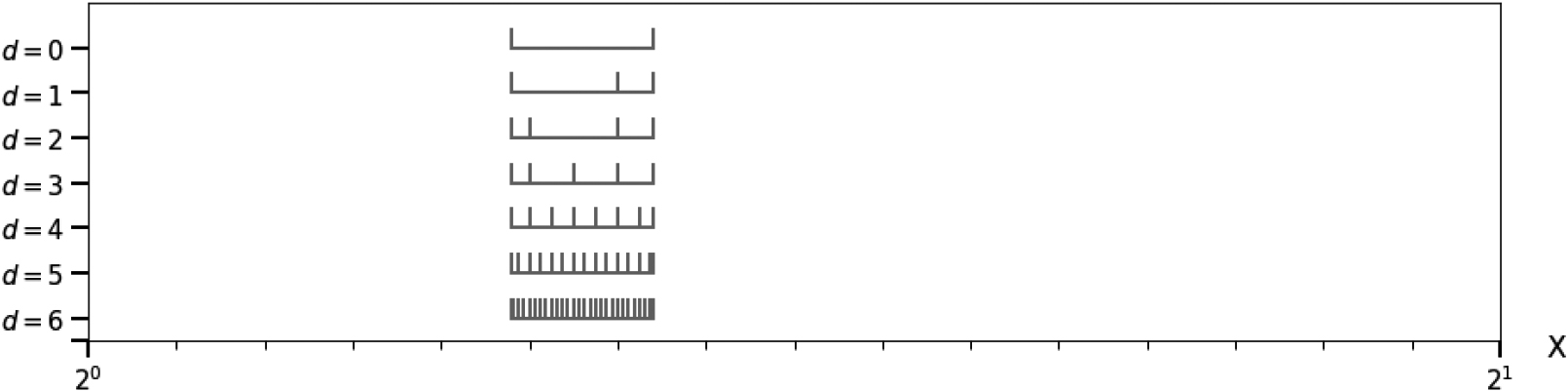

Let us consider a data set with values in $[1.3,1.4]$ . Only one exponent bin $B_{E+,0}=[2^{0},2^{1}]$ is enough to cover the data set. Within this exponent bin, the smallest mantissa bin that covers the whole data set is $[1.25,1.5]$ , with a mantissa precision $m=2$ . This allows to choose a set a mantissa bins at precision 32 ( $d_{\max}+m=30+2$ ) to cover our data set in a range $[c_{\min},c_{\max}]$ , with $|c_{\min}-1.3|<2^{-32}$ and $|c_{\max}-1.4|<2^{-32}$ . For $d=30$ , all the bins have the same length $2^{-32}$ and the total number of bins is $G_{30}=(c_{\max}-c_{\min})/2^{-32}<2^{30}$ . As the whole data set is contained in one single main bin, all the granulated bins have the same length $2^{-2-d}$ at any depth $d$ , except for the two extrema bins that need to be intersected with $[c_{\min},c_{\max}]$ . This is illustrated in Fig. 2, which shows the partition of the value domain in granulated bins for depths ranging from 0 to 6. For $d=0$ , there one single root bin $[c_{\min},c_{\max}]$ . For $d=1$ , two mantissa bins of length $2^{-3}$ , $[1.25,1.375]$ and $[1.375,1.5]$ are used, resulting in two granulated bins $[c_{\min},1.375]$ and $[1.375,c_{\max}]$ .

Example with multiple main bins

Let us consider a data set with values in $[-3,5]$ , and where the smallest non-zero absolute value is 0.15. We have $x_{\min}=-3,x_{\max}=5,i_{\min}=1,i_{\max}=2$ and $i_{*}=-3$ (as $2^{-3}<0.15\leqslant 2^{-2}$ ). The value domain is covered using five negative exponent bins $[-2^{2},-2^{1}]$ , $[-2^{1},-2^{0}]$ , $[-2^{0},-2^{-1}]$ , $[-2^{-1},-2^{-2}]$ , $[-2^{-2},-2^{-3}]$ , six positive exponent bins $[2^{-3},2^{-2}]$ , $[2^{-2},2^{-1}]$ , $[2^{-1},2^{0}]$ , $[2^{0},2^{1}]$ , $[2^{1},2^{2}]$ , $[2^{2},2^{3}]$ , plus two central bins $[-2^{-3},0]$ , $[0,2^{-3}]$ . Altogether, $n_{B}=13$ main bins are used, and for $d=4$ , the granulated bins consist of these $G_{4}=13$ bins. For $4<d\leqslant 0$ , the mains bins are grouped by 2, 4, 8, 16, leading to $G_{3}=7,G_{2}=4,G_{1}=2,G_{0}=1$ granulated bins. Conversely, for $d\geqslant 5$ , the main bins are split into mantissa bins exploiting $d-4$ digits for the precision of the mantissa. This is illustrated in Fig. 3, which shows the partition of the value domain in granulated bins for depths ranging from 0 to 6. For $d=2^{30}$ , each exponent or central bin is divided into $2^{26}$ equal-width mantissa bins, ranging from the smallest absolute length $2^{-29}$ in $[-0.25,0.25]=[-2^{-2},-2^{-3}]\cup[-2^{-3},0]\cup[0,2^{-3}]\cup[-2^{-3},-2^{-2}]$ to the largest absolute length $2^{-24}$ in $[4,5]$ .

Figure 3.

Granulated bins in case of multiple main bins.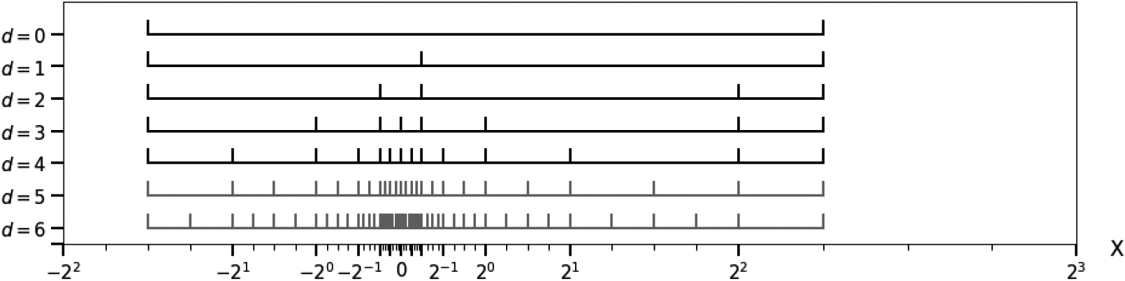

Figure 4.

Granulated bins in case of multiple main bins, using a logarithmic scale.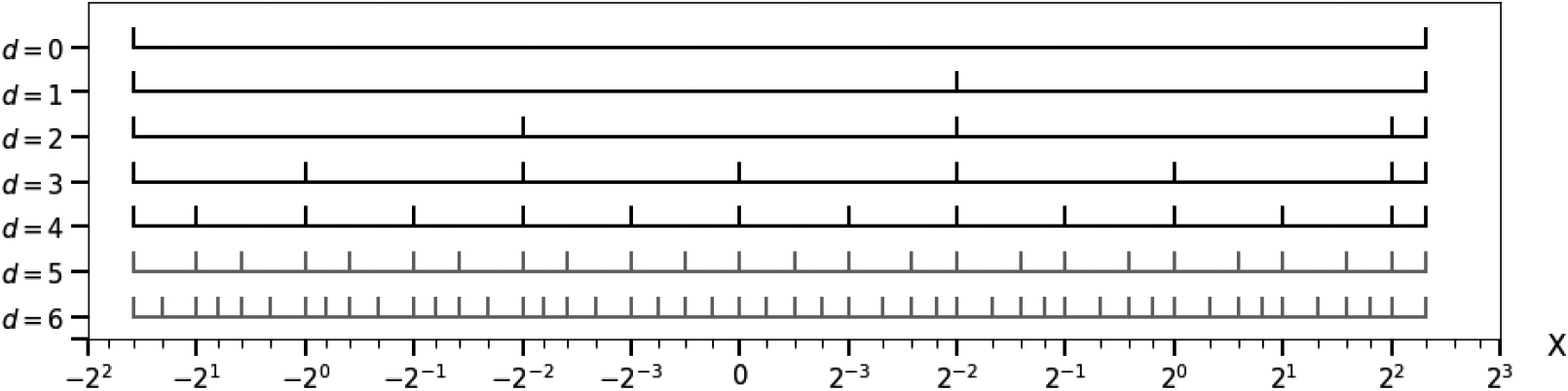

Figure 4 presents an alternative view of Fig. 3, keeping the linear scale within the central bins and exploiting a logarithmic scale for the negative and positive exponent bins. This shows that the lengths of the granulated bins are quite balanced when the relative precision of the interval boundaries is considered rather than their absolute precision. This also suggests an appealing visualization for histograms related to data sets with a dynamic range of values both in the negative and positive domains.

5. G-Enum-fp histogram method

In the previous section, we have exploited the floating-point representation of real values to introduce an alternative definition of the elementary bins used as building blocks for a new histogram method called G-Enum-fp. We first summarize the principles of this new method, then summarize its specific components.

5.1 Principle

The G-Enum method exploits a representation space based on elementary equal-width bins, using a granularity parameter $G$ to explore simplified versions of this representation space. It exploits these elementary bins as building blocks that provide a set of predefined bounds, from which the bounds of the histogram intervals are chosen.

The main novelty of the G-Enum-fp method is to replace the elementary equal-width bins of G-Enum with the floating-point bins and their granulated hierarchy introduced in Section 4. This makes a radical difference regarding the impact of the granularity parameter $G,1\leqslant G\leqslant E$ :

with the G-Enum method, $E=10^{9}$ is considered huge, but it sets a limit of one billionth of the value domain for the smallest interval, which is harmful in event of outliers (see Section 3.1),

with the G-Enum-fp method and the same $E$ , this limit is extended by more than six hundred orders of magnitude (see Section B.2).

In addition to this major change, the G-Enum-fp method extends the modeling space and the optimization algorithms of the G-Enum method to take full account of the particularities of floating-point bins. To begin with, the bounds of the entire numerical domain are explicitly specified as hyper-parameters. The other difference related to the floating-point representation is the management of the singularity around 0, which relies on the choice of a central bin, treated as an additional model parameter. These extensions are summarized in the following subsections and detailed in Appendix A. Some properties of the G-Enum-fp method are also discussed in Appendix B.

5.2 Specification of domain bounds

With the G-Enum method, the domain bounds are implicitly derived from the data using $[x_{\min}-\epsilon/2,x_{\max}+\epsilon/2]$ . With the G-Enum-fp method, the domain lower and upper bounds are explicitly defined using hyper-parameters that belong to the modeling space:

main bin containing the domain lower bound,

main bin containing the domain upper bound,

central bin exponent of the domain if necessary,

digit precision used for mantissa bins,

mantissa bins containing the domain bounds.

These domain lower and upper bounds are inferred once for all, before optimizing the histogram. An evaluation criterion is obtained using a MDL-based approach. Its optimization consist of two steps:

recover the extreme values $x_{\min}$ and $x_{\max}$ using a loop over the data set in $O(n)$ ,

encode a lower bound of $x_{\min}$ and an upper bound of $x_{\max}$ using the floating-point representation and optimize the number of digits used for the mantissa, in $O(r_{m})$ where $r_{m}=52$ is the maximum number of bits in the mantissa.

The details regarding the specification and optimization of these hyper-parameters are given in Appendix A.2.

5.3 Choice of the central bin

With the G-Enum-fp method, we introduce a new parameter $i_{\textit{cen}}$ to choose the exponent of the central bin used to obtain a representation space based on floating-point bins. In fact, we can choose any value of $i_{\textit{cen}}$ that conforms with the domain bounds, between $i_{\textit{cen}_{\min}}$ corresponding to the central bin exponent of the domain, and $i_{\textit{cen}_{\max}}$ which allows us to contain the domain lower and upper bounds. With $i_{\textit{cen}}=i_{\textit{cen}_{\min}}$ , we obtain a maximally floating-point representation, as the related exponent bins extends over a wide range of values. With $i_{\textit{cen}}=i_{\textit{cen}_{\max}}$ , we obtain a maximally equal-width representation, as the bins considered are of equal-width.

Optimizing the exponent of the central bin is mainly a matter of calling the G-Enum optimization algorithm twice, keeping its overall computational complexity:

optimize a first histogram $M(i_{\textit{cen}_{\min}})$ for $i_{\textit{cen}}=i_{\textit{cen}_{\min}}$ , corresponding to the maximally floating-point representation,

search for the largest value $i_{\textit{cen}_{\textit{opt}}}$ of $i_{\textit{cen}}$ in $[i_{\textit{cen}_{\min}},i_{\textit{cen}_{\max}}]$ which maintains the same partition of the data set into intervals as in $M(i_{\textit{cen}_{\min}})$ , with interval endpoints recoded on the basis of $i_{\textit{cen}_{\textit{opt}}}$ ,

optimize a second histogram $M(i_{\textit{cen}_{\textit{opt}}})$ for $i_{\textit{cen}}=i_{\textit{cen}_{\textit{opt}}}$ and keep this histogram if its evaluation criterion is better than that of the first histogram.

The introduction of this new parameter $i_{\textit{cen}}$ and its optimization are detailed in Section A.3.

5.4 G-Enum-fp criterion

Table 2
G-Enum-fp criterion

Criterion	Indexing terms	Multinomial terms	Bin index terms
G-Enum-fp	$\log^{}(1+i_{\textit{cen}_{\max}}-i_{\textit{cen}})+\log^{}K+\log^{*}(1+d)$	$\log\left(\begin{array}[]{c}{n+K-1}\\ {K-1}\end{array}\right)$	$\sum^{K}_{k=1}{h_{k}\log E_{k}}$
	${}+\log\left(\begin{array}[]{c}{G_{d}+K-1}\\ {K-1}\end{array}\right)$	${}+\log\frac{n!}{h_{1}!\ldots h_{K}!}$

Table 2 shows the G-Enum-fp criterion for the parameters of histogram models. Compared with the G-Enum criterion recalled in Table 1, the only differences concern the indexing terms:

the term $\log^{*}(1+i_{\textit{cen}_{\max}}-i_{\textit{cen}})$ is used to encode the new parameter $i_{\textit{cen}}$ ,

the exponent $d$ of the granularity ( $G=2^{d}$ ) is encoded instead of the granularity $G$ itself,

the exact number of considered floating-point bins $G_{d},2^{d-1}<G_{d}\leqslant 2^{d}$ at a given granularity is used instead of $G=2^{d}$ in the case of equal-width bins.

In addition, new hyper-parameters have been introduced for the domain bounds (see Table 4 for the corresponding criterion). Note that the G-Enum-fp method is parameter-free, as all its parameters and hyper-parameters belong to the modeling space.

6. Experiments with artificial data sets

In this section, we evaluate the G-Enum-fp method using artificial data sets with known underlying data distribution. We focus on resistance to outliers and heavy-tailed distribution, beyond the limits of state-of-the art methods. A binary standalone implementation of the method is available here: http://marc-boulle.fr/khisto/.

6.1 Evaluation protocol

Metrics

The accuracy of histograms for density estimation is evaluated using the Hellinger distance to the original model density, which is known in the case of artificial data sets. The Hellinger Distance (HD) $H(p,q)$ for $p, q$ being probability density functions, is defined as

$\displaystyle H(p,q)=\frac{1}{\sqrt{2}}\sqrt{\int(\sqrt{p(x)}-\sqrt{q(x)})^{2}% }dx$

A HD close to 0 indicates a strong similarity between probability distributions. The HD measures reported are obtained via numerical integration to estimate the probability distributions of the model density and of the histogram that models it.

The number of intervals per histogram is also collected.

Histogram methods

Histogram methods are limited in the case of outliers or heavy-tailed distribution, as indicated in Section 3. We evaluate the G-Enum-fp method in these challenging cases. We also report the results obtained by the G-Enum method, chosen as a strong baseline, especially in the case of heavy-tailed distributions and large data sets (cf Section 2.5). Since our aim is to push the limits of histograms with data set sizes and value domain widths several orders of magnitude larger than those evaluated in [6], the G-Enum method is in fact the most appropriate method that can be used for comparison purposes.

Data sets

As a sanity check, we first evaluate the behavior of the methods in the case of common distributions, using the uniform, normal and a mixture of normal distributions. The results of these experiments are presented in Appendix C. We then analyze the case of data sets with outliers and heavy-tailed distributions using the Lévy distribution and a pathological mixture of lognormal distributions. The results of these experiments are presented in the following subsections.

6.2 Normal distribution with an outlier

The objective of this experiment is to evaluate the impact of an outlier on the quality of the built histograms. We exploit a data set of size $n=10,000$ generated from a normal distribution $\mathcal{N}(1,0.1)$ . We add one outlier with value $v_{\textit{out}}=2^{i},0\leqslant i\leqslant 34$ from $v_{\textit{out}}=1$ to $v_{\textit{out}}=2^{34}\approx 1.7\;10^{10}$ . The experience is repeated 100 times, which represents 3,500 data sets. We collect the Hellinger distance and number of intervals. The Hellinger distance is computed using the underlying $\mathcal{N}(1,0.1)$ distribution, assuming that the impact of one outlier among $n=10,000$ instance should be negligible.

Figure 5.

Hellinger distance and number of intervals for 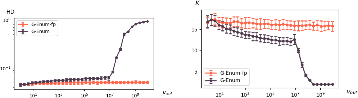$\mathcal{N}(1,0.1)$ with an outlier.

The overall results are reported in Fig. 5. They show that the G-Enum is rather resilient to the outlier on a large scale of values, up to about $10^{7}$ , that is more than one million times the range of values of the underlying distribution. The built histograms have a slowly decreasing quality, from around 17 intervals without outlier, down to 12 intervals for $v_{\textit{out}}\approx 10^{7}$ . For more distant outliers, the $10^{9}$ equal-width elementary bins are no longer sufficient to accurately estimate the underlying distribution. In the end, the histogram consists of two intervals, the first one exploiting one single elementary $\epsilon$ -length bin and containing all the normal values, the second one containing only the outlier.

The G-Enum-fp method benefits from its floating-point representation to be highly resilient to the outlier. Beyond $v_{\textit{out}}>2$ , the G-Enum-fp method always exploits the maximally floating-point representation corresponding to a minimum central bin exponent. As the outlier becomes more distant, the G-Enum-fp method exploits an increasing number of exponent bins, up to around 35 for the largest outlier value $v_{\textit{out}}=2^{34}$ . The first exponent bins can then be split accurately into mantissa bins, allowing an accurate approximation of the underlying density whatever be the distance of the outlier, which is contained alone in one large interval. We conducted additional experiments with a googol outlier ( $v_{\textit{out}}=10^{100}$ ). The number of exponent bins necessary to cover the value domain increases up to 334, resulting in largest cost for the prior terms of the G-Enum-fp. The method is still very accurate, using 14 intervals to approximate the normal distribution plus the outlier, instead of 15 for $v_{\textit{out}}=10^{10}$ .

6.3 Lévy distribution

The objective of this experiment is to compare the behavior of the methods in the case of a heavy-tailed distribution. We exploit the Lévy distribution that is pathological, having neither mean nor variance. We also evaluate the scalability of the methods, by generating samples of size $n=10^{i},1\leqslant i\leqslant 9$ . Note that the range of data set values increases very quickly with the sample size, with maximum values greater than $10^{18}$ for one billion data points. The experiment is repeated 10 times and we collect the Hellinger distance and number of intervals per sample size.

Figure 6.

Hellinger distance and number of intervals for a Lévy distribution.

The overall results are reported in Fig. 6. The G-Enum method is not able to produce an accurate approximation of the underlying density for $n$ above $10^{3}$ . Beyond this threshold, even $10^{9}$ equal-width elementary bins are not sufficient to approximate accurately the Lévy distribution. Indeed, the bins necessary to cover the tails of the distribution become too large for a correct approximation around the median value, which contains most of the probability mass.

The G-Enum-fp method exploits up to 66 exponent bins to cover the huge range of values for $n=10^{9}$ , and it keeps an approximately constant relative precision with its mantissa bins, whatever be the position of the interval boundaries. It is able to continuously improve the approximation of the underlying density as $n$ increases, building more and more intervals.

Figure 7 shows an example of the histograms obtained by each method for $n=10^{9}$ . The histograms are displayed using a $\log\times\log$ scale for the interval boundaries on the $X$ axis and their densities of the $Y$ axis. The G-Enum-fp histogram that accurately approximates the Lévy distribution consists of 1,253 intervals with lengths ranging from $6.1\times 10^{-4}$ to $2.3\times 10^{18}$ , frequencies from 8 to $16.03\times 10^{6}$ and densities $3.4\times 10^{-27}$ to 0.46.

Figure 7.

Density and histograms for a Lévy distribution, with 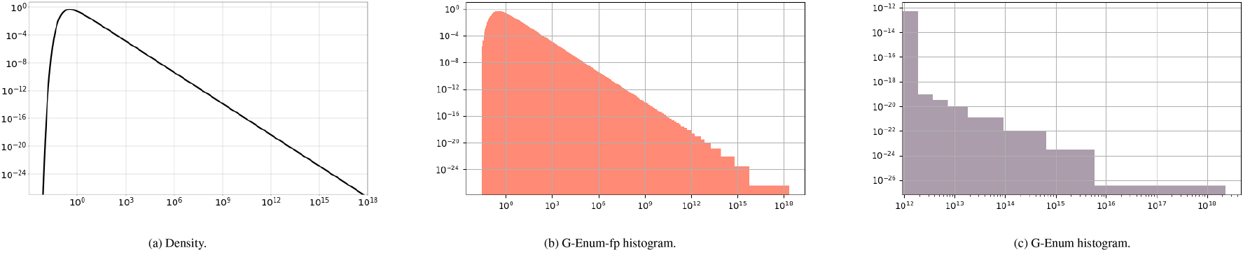$n=10^{9}$ .

6.4 Lognormal mixture distribution

The objective of this last experiment is to push the G-Enum-fp to its limits, using a pathological mixture of heavy-tailed distributions. We generate data sets of size $n=10^{i},1\leqslant i\leqslant 9$ using a mixture of ten lognormal distributions.

$\displaystyle\sum_{i=1}^{10}{\frac{1}{10}\log\mathcal{N}(10^{i},\sqrt[10]{10^{% i}})}$ (1)

Figure 8.

Number of intervals for a mixture of lognormal distributions.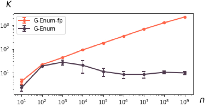

The experiment is repeated 10 times and Table 9 reports the mean and standard deviation of the number of intervals per sample size. With this pathological distribution, the range of values is enormous, from $10^{1}$ to $10^{24}$ for data sets with one billion data points, and we were unable to calculate the Hellinger distance due to numerical problems. Due to this huge range of values, the G-Enum method fails to correctly approximate the underlying distribution and ends with histograms containing about ten intervals. On the opposite, as with the Lévy distribution, the G-Enum-fp method continuously improves the approximation of the underlying density as $n$ increases, building more and more intervals.

Figure 9.

Density and histograms for a mixture of lognormal distributions, with $n=10^{9}$ .

Figure 9 displays an example of the histograms obtained by each method for $n=10^{9}$ . The G-Enum-fp histogram that accurately approximates the underlying distribution consists of 2,295 intervals with lengths ranging from $4.8\times 10^{-4}$ to $2.6\times 10^{24}$ , frequencies from 8 to 90.5 million and densities $3.0\times 10^{-33}$ to 0.13.

7. Histograms for exploratory analysis

In this section, we apply the G-Enum-fp method to real-world data sets. However, histograms may not be directly useful for the exploratory analysis of real data, as shown in a first example. We then propose heuristics to better process real data and suggest a methodology for using histograms in the context of exploratory analysis. This methodology is illustrated using some standard data sets.

7.1 Applying histograms to real-world data sets

We apply the G-Enum-fp method to the petal length variable of the iris data set [16]. The obtained histogram is presented in Fig. 10

Figure 10.

Iris petal length histogram, with the density on a linear scale (left) and a logarithmic scale (right).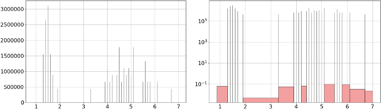

The resulting combed histogram consists of 51 intervals, 25 of them containing one single value and of width $3\times 10^{-8}$ . In fact, the G-Enum-fp method is a density estimator, and it reveals that the iris data set consists mostly of discrete data, leading to a list of density peaks. This is actually a good density estimate, as the petal length variable is recorded with a decimal precision of 0.1, with the 150 instances containing only 43 distinct values.

However, this combed histogram is not very useful for exploratory analysis. Usually, this problem of truncated data is solved by practitioners by setting an adequate minimum bin width, the truncation gap, for the histogram intervals. This can be a tricky task for new data for which there is no prior knowledge to guess this truncation gap, and tedious trial and error testing may be required.

7.2 Heuristic to deal with truncated data

We propose an adaptation of the G-Enum-fp method to process integer data, then a heuristic to automatically process truncated data.

7.2.1 Dealing with integer data

First, note that all integers $n$ that can be represented on a computer belong to floating-point bins $[n-1,n]$ : either the central bins $[-2^{0},0]$ and $[0,2^{0}]$ , the exponent bins $[-2^{1},-2^{0}]$ and $[2^{0},2^{1}]$ , or mantissa bins of width at least $2^{0}$ for the exponent bins with larger exponents. To adapt the G-Enum-fp method to integer data, we suggest to exploit the subset of floating-point bins that are compatible with integers, that is all floating-point bins larger than 1. There are few impacts on the G-Enum-fp method:

the domain bounds represented by the hyper-parameters need to be integers,

the exponent of the central bin is at least 0,

the granulated bins are constrained to be of width at least 1.

In the main algorithm (cf. Section A.4), at each depth $d$ of the hierarchy of granulated bins, the main bins of width $2^{e},e\geqslant 0$ are split into $\max(2^{d},2^{e})$ granulated bin. This results in a lower value of $G_{d}$ , the number of granulated bins $G_{d}$ that cover the data set, in the indexing terms of the G-Enum-fp criterion. Apart from these changes concerning the granulated bins to consider and the value of $G_{d}$ , the method is the same.

This extension of G-Enum-fp to integer data allows to process truncated data with a truncation gap of 1, which translates into floating-point bins with a minimum width of $2^{0}$ . Note this can be applied in the same way to any floating bins of width at least $2^{i}$ , to process any truncated data which truncation gap is a power of two.

7.2.2 Dealing with truncated data

Our objective is to automatically process truncated data to facilitate the task of exploratory analysis. We then suggest a three-steps truncation management heuristic (TMH):

detection of truncated data,

calculation of the truncation gap,

construction of a histogram adapted to truncated data.

Detection of truncated data

Let us define a peak as a histogram interval which density is greater than that of its previous and next intervals, a spike as a peak containing one single value and a singularity as a spike which previous and next intervals are empty. For example, the combed histogram in Fig. 10 contains 25 spikes, 14 of which being singularities. We assume that spikes are a signature of truncated data and choose to trigger the next steps in the presence of at least one spike. We expect this very simple criterion to correctly identify most of the relevant cases while avoiding unnecessary additional computation time in the other cases.

Calculation of the truncation gap

After sorting the $n$ data entries $x_{1},\ldots,x_{n}$ by increasing values, we collect the $(n-1)$ variations of values $\delta x_{i}=x_{i+1}-x_{i},1\leqslant i\leqslant n-1,$ and compute a histogram from these variations of values.

Figure 11.

Histogram of variations of values for petal length.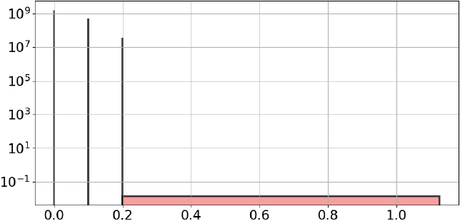

As an example, the resulting variation histogram is shown in Fig. 11 in the case the petal length variable of the iris data set. We propose to detect the following truncation pattern within the variation histogram to confirm whether the data is truncated:

the first interval contain only the value 0,

the second interval is empty,

the third interval has a strictly smaller length than the second interval.

This pattern is present in Fig. 11, which contains two spikes related to the variation of values 0.1 and 0.2. Note than we do not impose that the third interval of the variation histogram be a spike, in order to be resilient to potential rounding errors. We finally exploit the truncation pattern to calculate the truncation gap, as the mean value contained in the third interval, that is the averaged minimum distance between two consecutive distinct values.

Construction of a histogram adapted to truncated data

If a non-zero truncation gap $\gamma_{t}$ is available, we exploit the adaptation of the the G-Enum-fp method to integer data described in Section 7.2.1. We first choose a binary truncation gap $\gamma_{bt}$ as close as possible to the truncation gap, according to $\gamma_{bt}=2^{i_{bt}}$ with $i_{bt}=\lceil\log_{2}(\gamma_{t})\rceil$ . We then transform the initial data so that they conform to the binary truncation gap, then we compute the histogram using the method described in Section 7.2.1 with a minimum floating bin of width $\gamma_{bt}$ , and finally reverse transform the obtained interval bounds to conform with the initial value domain.

To transform the initial data and get values that are all multiples of the binary truncation gap, we project the data on the upper bounds of the floating-point bins of width $\gamma_{bt}$ that contain each data entry:

$\displaystyle y_{i}=\lceil x_{i}/\gamma_{t}-1/2\rceil\gamma_{bt}.$ (2)

Symmetrically, the reverse transformation of the interval bounds is calculated using

$\displaystyle x_{i}=(y_{i}/\gamma_{bt}+1/2)\gamma_{t}.$ (3)

Figure 12.

Iris petal length histogram, taking into account truncated data.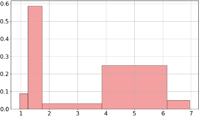

For example, the obtained histogram related to the petal length variable of the iris data set is presented in Fig. 12. It consists in five intervals, which looks reasonable given that the data set contains only 150 data entries. Its shape seems consistent with the knowledge available concerning the iris data set. It is mixture a three classes of iris flowers, setosa, versicolor and virginica, of small, medium and large sizes, with the petal lengths in $[1.0,1.9]$ for setosa, in $[3.0,5.1]$ for versicolor and in $[4.5,6.9]$ for virginica.

7.3 Methodology for exploratory analysis

Our first objective in this paper was to devise a histogram method that could be applied automatically for the exploratory analysis of any real-world data set. While this goal seems attained in the case of artificial data set where the data generation process is controlled (see Section 6), it may not be achievable with real-world data sets. During the digitization process, the data may exhibit a wide range of tricky patterns beyond rounding or truncation issues, meaning that

“the digitized structure of the data is a much more robust feature than the statistical structure of the original data. In such cases, an uninvertible transformation has been applied to the data, and information has been irrevocably lost.” [17]

The method based on an optimal histogram algorithm [17] allows to identify digitization problems, which is useful as “it may be desirable for researchers to know that information has been discarded”. Beyond this useful feature, our relaxed goal is to help the data analyst filter the digitized structure of the data and discover its statistical structure. We suggest first computing a series a histograms of varying granularities, the finest grain allowing to discover local patterns and the coarsest grain allowing to focus on global patterns. We then provide a list a indicators per histogram to facilitate the task of exploratory analysis.

It is worth noting that this methodology may also be used with other histogram methods. However, its deep integration with the G-Enum-fp method brings several interesting advantages: resistance to outliers and heavy-tailed distributions (cf. Section 6), fine-tuning of the criterion and algorithms in the case of truncated data (cf. Section 7.2.1), and reuse of the intermediate histograms obtained at each depth of granularity as a by-product of the main G-Enum-fp optimization algorithm (cf. Section 7.3.1).

7.3.1 Series of histograms

We optimize a first histogram using the G-Enum-fp method and keep it even in the case of singularities, as it may bring some information regarding digitization problems (as in [17]). We then apply the TMH heuristic to build an adequate histogram if the data are detected as truncated. The current histogram, obtained for an optimal depth of granularity $d_{\textit{opt}}$ , can be seen at coarser grains for all the intermediate depths $d$ , $0\leqslant d\leqslant d_{\textit{opt}}$ : we collect all these intermediate histograms evaluated along the optimization trajectory. In order to focus on interpretability and to automatize the exploratory analysis as much as possible, we apply a singularity removal heuristic (SRH) by discarding the finest grained histograms having singularities (spikes with two surrounding empty intervals). We could relax the removal criterion by considering spikes or even empty intervals, but this might destroy some potentially useful information.

To summarize, we get a list of interpretable histograms by decreasing depth of granularity, $d_{\textit{opt}_{\textit{inter}}}\geqslant d\geqslant 0$ , plus potentially a raw histogram if the first optimized histogram was not interpretable.

7.3.2 Indicators per histogram

To facilitate the exploration of the list of interpretable histograms, we provide the following indicators based on elementary patterns: number of intervals, peaks, spikes and empty intervals. We also introduce a last indicator based on the level-fp criterion (see Section B.4) that is the percentage of information kept in an interpretable histogram compared to the finest grained interpretable histogram:

$\displaystyle\text{\%information}(M)=\frac{\text{level-fp}(M)}{\text{level-fp}% (M_{d_{\textit{opt}_{\textit{inter}}}})}.$ (4)

7.4 Illustration

We illustrate the exploratory analysis methodology introduced in this section using some simple data sets. Extensive evaluation is performed in Section 8.

7.4.1 Old faithful geyser

This data set contains 272 data entries related to eruptions of the Old Faithful geyser [18], with duration and waiting time between eruptions. The duration is used in [9] to illustrate the difficulties of correctly identifying density peaks applying automatic histogram methods on heavily rounded real data. Whereas histograms with two peaks are usually expected, nine automatic histogram methods evaluated in [9] largely disagree on the shape of the histogram, building 5, 11, 19, 23, 37, 42, 111, 143 or 149 intervals.

Similarly, the G-Enum-fp method fails to identify the underlying statistical pattern and reveals the digitization structure with a histogram having 71 intervals, including 35 spikes. The TMH method identifies a truncation gap of 0.001 and outputs the interpretable histogram shown in Fig. 13a. Its contains two density peaks as expected, and its shape seems to correspond with the underlying statistical density, as suggested by a visual inspection of the scatterplot in Fig. 13b.

Figure 13.

Old faithful geyser.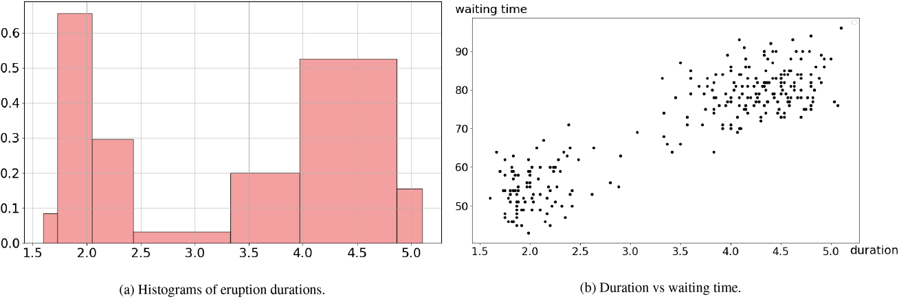

Note that the truncation pattern seems rather surprising for this data set, as only two pairs of successive values are separated by 0.001, while 31 are separated by 0.016 and 57 by 0.017. As $1/60\approx=0.0166$ and after inspecting the data in their plain text format, we assume that the data were recorded with a precision of one second, then transformed to decimal minutes according to $x=m+s/60$ and finally truncated using 3 decimal digits. The digitization process thus includes three steps: recording of observations with limited precision, transformation then truncation of the data. This leads to fine-grained digitization patterns that dominate the underlying statistical patterns. Using the methodology suggested in Section 7.3 provides useful information and allows to recover the statistical structure of the data beyond their digitization structure.

7.4.2 Adult

The adult data set [16] contains 48,842 data entries extracted from a census database. We apply our method to the age variable, which is an integer variable as ages are commonly recorded with one year precision. The G-Enum-fp method builds a raw histogram with 143 intervals, 70 of which being spikes, including 67 singularities. The TMH method correctly identifies a truncation gap of 1 and outputs the interpretable histogram shown in Fig. 14.

Figure 14.

Age in adult data set.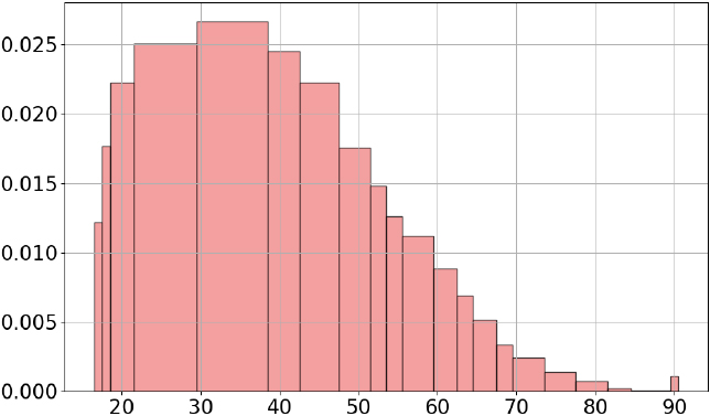

Note that there is a surprising increase of density at age 90. This pattern is confirmed by a close examination of the three last intervals of the histogram, with 39 people between 82 and 84 years of age, 17 between 85 and 89 years of age, and 55 for 90 years of age, the maximum age in the data set. This may indicate that people over the age of 90 were all recorded with the age of 90.

Discussion

For illustration purposes, the raw histogram obtained before applying the TMH heuristic is shown in Fig. 15a. This raw histogram is a very accurate density estimator for this data set containing 48,842 data entries for only 74 distinct values. All ages except two are distributed in bins of very small width separated by empty bins almost a year wide. The two exceptions contains too few data entries to be isolated: one data entry for age 86 and two for age 89. Although this histogram is very accurate, it is of little interest for exploratory data analysis.

A regular histogram with a suitably chosen equal-width (value 1 year) is also presented in Fig. 15b. It gives the overall shape of the data, but is very noisy, compared to the interpretable histogram obtained using the TMH heuristic (see Fig. 14) which recovers a smooth version of the distribution.

Let us note that histograms for mixed discrete-continuous data have been proposed [19], with a user-defined threshold (e.g. 5) for detecting discrete values and a histogram method for the rest of the data. In the case of the adult data set, this approach would result in a histogram similar to that shown in Fig. 15a, as most values would be detected as discrete. It is not suitable in the case of truncated data, where the discrete nature of the data is an artifact of the digitization process, masking the underlying statistical patterns of interest.

Figure 15.

Raw histogram (log scale) and regular histogram (equal-width 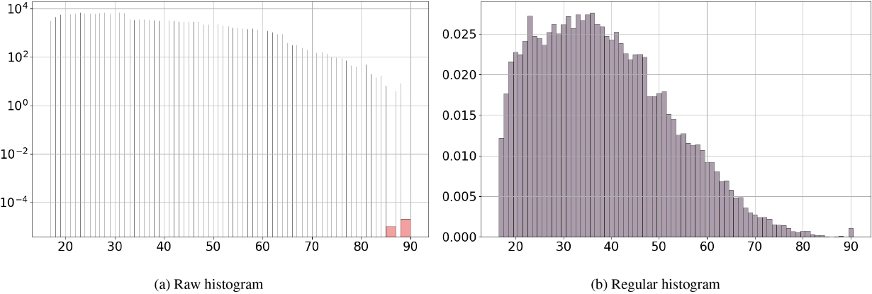$=$ 1) of age in adult data set.

7.4.3 Forest cover type

The forest cover type data set [16] contains 581,012 observations ( $30\times 30$ meter cells) from a geological survey. We analyze the variable horizontal distance to nearest roadway. The raw histogram contains 10,992 intervals, revealing serious digitization issues. The TMH method correctly identifies a truncation gap of 1 related to a one meter precision, but it outputs a histogram that is still not interpretable, with 251 singularities. Once the SRH algorithm is applied to get the 1^st interpretable histogram, the result has a globally understandable, albeit comb-like shape, as shown in the Fig. 17a. In fact, these data suffer from at least two effects of digitization. The data are recorded with a precision of one meter, which is rather accurate but results in the accumulation of data entries around integer values. And the nature of the observations, based on a mesh of square cells of $30\times 30$ meters, is likely to introduce local correlations.

Figure 16.

Forest cover type: Indicators per depth of granularity.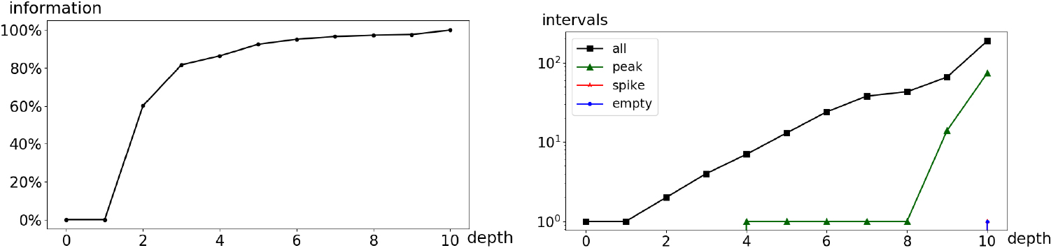

Applying the methodology introduced in Section 7.3, a series of histograms is collected for all the coarse-grained depths of granularities, starting from the 1^st interpretable. The indicators collected per histogram are displayed in Fig. 16. They suggest to exploit a two times coarsened histogram to eliminate the comb-like pattern while preserving most of the information. The resulting unimodal histogram shown in Fig. 17b is rather smooth and suitable for an easy interpretation, while keeping 98.9% of the information.

Figure 17.

Horizontal distance to nearest roadway in forest cover type data set.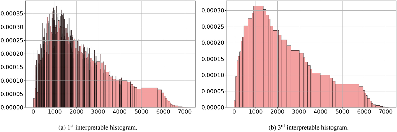

8. Evaluation with large scale real-world data sets

In this section, we evaluate the floating-point histograms as well as the methodology introduced in this paper for exploratory data analysis, using several large scale real-world data sets.

8.1 Evaluation protocol

Histograms are widely used in exploratory data analysis (EDA) [20] as visualization tools in the data discovery process. However, in the case of challenging real-world data sets, they are difficult to use in practice. Even state-of-the-art histograms are hardly usable in the following cases:

they reach their limit in the case of outliers or heavy-tailed distributions (cf. Section 3),

they produce accurate but useless comb-shaped histograms in the case of truncated data (cf. Section 7.4.2),

they cannot scale with very large data sets or very large value domains (cf. Section 2.5).

The purpose of this section is to assess whether the proposed exploratory methodology, based on the G-Enum-fp method, is capable of pushing the limits of the effective use of histograms for EDA. The approach is evaluated using several real world data set that combine multiple challenges: heavy-tailed distribution, integer data, large scale, complex patterns. As there is no ground truth in EDA, the evaluation cannot be measured objectively. Instead, the patterns recovered using the proposed approach are compared to the prior knowledge available for each data set.

Figure 18.

Moon crater Salamuniccar: indicators per depth of granularity.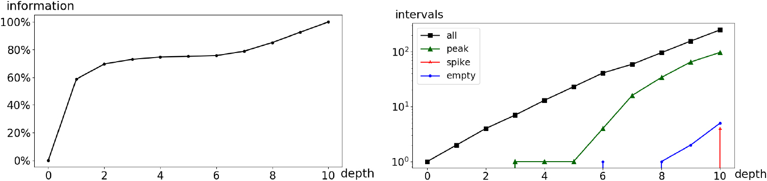

Figure 19.

Moon crater Salamuniccar database.

8.2 Moon crater Salamuniccar database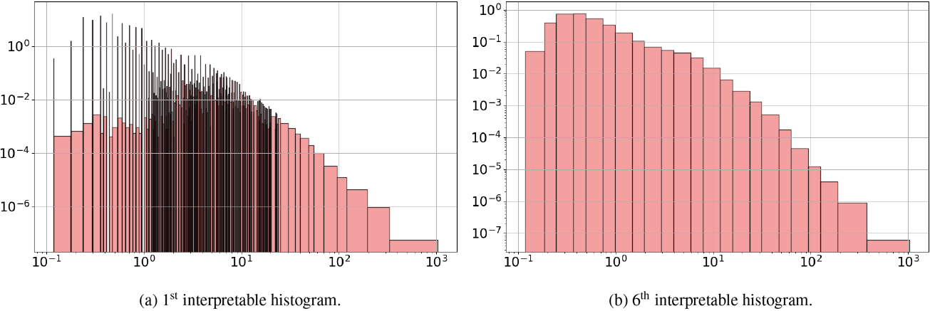

The moon crater Salamuniccar database [21]2 is a catalog of 78,287 lunar crater impacts. We exploit this database to analyze the distribution of the radius of the craters. The raw histogram output by the G-Enum-fp method contains 2,497 intervals, including 1,204 spikes and 325 singularities. The TMH method identifies a truncation gap of $3\times 10^{-5}$ , which looks dubious, and the SRH method discards the 140 remaining singularities to obtain the 1^st “interpretable” histogram. This highly combed-shape histogram still contains 249 intervals, including 97 peaks, which is hardly useful for exploratory analysis. These numerous peaks could be explained by the data collection process described in [21], which states that the catalog is globally complete only for crater diameters greater than 8 km, and that the data were recorded using several instruments, some with an accuracy of about one meter and others with a resolution of about 100 meters/pixel. These characteristics are consistent with the data in their plain text format, which consist of less than 3,200 distinct values recorded to a decimal precision of 6 digits.

Applying the methodology introduced in Section 7.3, the indicators related to coarser-grained histograms are displayed in Fig. 18. They suggest using the 6^th histogram, obtained at depth 5, which is reduced to a unimodal distribution summarized with 23 intervals (see Fig. 19b). Even with this small number of intervals, the floating-point representation allows to recover a global shape in power law. Still, the information curve in Fig. 18 suggests a loss of information of more than 20% during this coarsening process, especially for crater diameters smaller than 10 km, as shown in Fig. 20. This is consistent with the data collection process and may caution the data analyst to avoid drawing too precise conclusions from this data set.

Figure 20.

Moon crater Salamuniccar database: intermediate histograms.

8.3 Moon crater Robbins database

The moon crater Robbins database [22]3 contains approximately 1.3 million lunar impact craters. This recent database is estimated to be a complete census of all craters larger than approximately 1 to 2 km. The G-Enum-fp method directly builds an accurate and smooth histogram with 87 intervals that looks easy to interpret, as shown in Fig. 21. It captures a power law decrease of the densities for craters between 1 km and 2,500 km, in line with astrophysics literature: power or multiple power laws are often used to fit the crater size distribution [23].

Figure 21.

Moon crater Robbins database.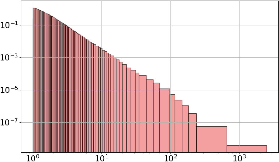

8.4 HYG stellar database

The HYG stellar database [22]4 contains 119,614 star records from three catalogs: Hipparcos, Yale Bright Star and Gliese. We exploit this database to analyze the distribution of stars’ luminosity, as multiples of the Solar luminosity. The raw histogram output by the G-Enum-fp method contains 17,032 intervals, including 8,513 spikes and 7,348 singularities (see Fig. 22a). Although the luminosity is recorded with an accuracy of 10 decimal digits, there are only 13,451 distinct values for 119,614 records, which explains the raw histogram with a very comb-like shape.

Figure 22.

HYG stellar database.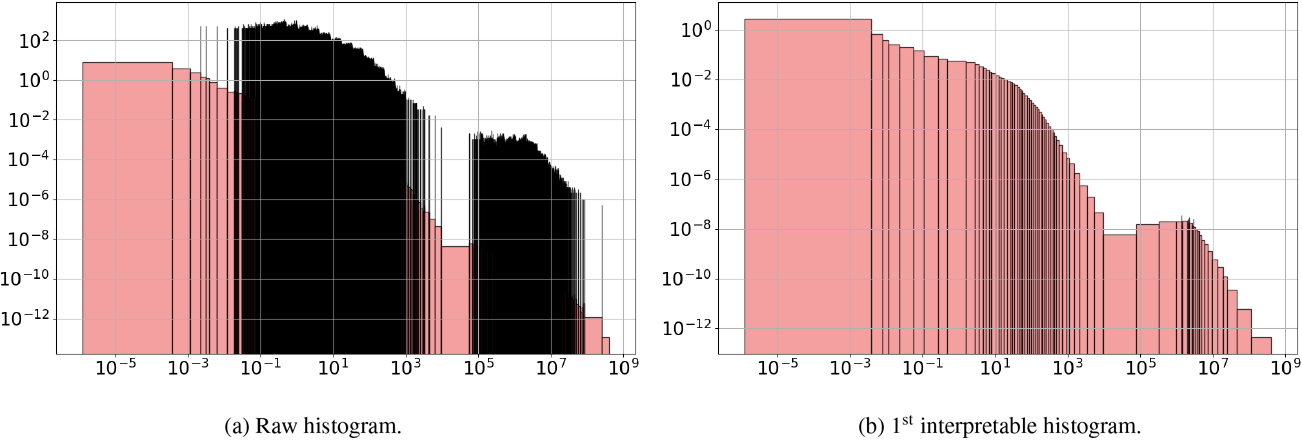

No truncation gap is identified, and the $1^{\text{st}}$ “interpretable” histogram obtained by the SRH method contains 81 intervals (see Fig. 22b). This histogram, which spans over 14 orders of magnitude, benefits from the floating-point representation of the G-Enum-fp method. It highlights an interesting smooth and precise distribution of the luminosity of the stars, with an approximate mixture of decreasing power laws. This overall irregular shape of the histogram probably comes from the data set, which is a mixture of three rather different catalogs. For example, the Yale Bright Star catalog contains essentially all stars visible with the naked eye, which may explain the “bump” at the end of the histogram. And conversely, the Gliese catalog is the most comprehensive catalog of nearby stars, that contains many fainter stars not found in Hipparcos.

8.5 Orange call detail records

The data set studied here is composed of nearly 25 million entries of cumulated call durations for incoming calls collected during one day, for a large sample of phone numbers of the Orange telecommunication company.5 The TMH method correctly identifies a truncation gap of 1 related to a one second precision and directly outputs the histogram displayed in Fig. 23, that consists of 222 intervals, with no singularity.

Figure 23.

Orange CDR.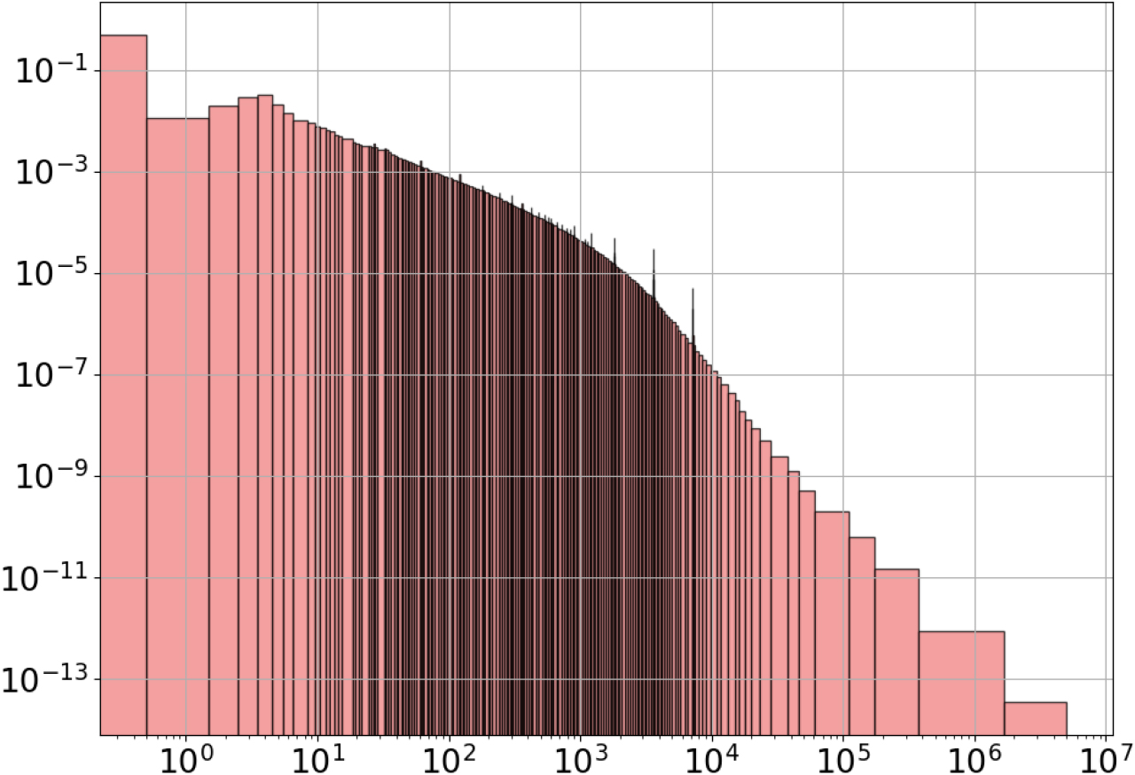

The fairly compact representation provided by this histogram summarizes a lot of information, beyond the overall shape of the distribution previously known as being heavy-tailed. For example, the first dense interval corresponds to phone numbers without any calls during the day, resulting in a cumulated call duration of 0 seconds. It spans over just one second but represents about half of the data set. Strikingly, the last interval covers about 3 million seconds and only accounts for 3 data entries, related to incoming calls collected one day that lasted more than one month. Another finding is that the heavy-tailed form exhibits two distinct power-law regimes, with a transition for durations of around one hour.

While the histogram looks globally smooth, there still are several dense peaks in-between. One could apply the methodology introduced in Section 7.3 to treat these peaks as digitization patterns and discard them, but they seem to be robust patterns that can only be eliminated after coarsening the histogram almost ten times. The three most notable peaks in the right (in the range $[10^{3};10^{4}]$ of Fig. 23) correspond to call durations of exactly 1800, 3600 and 7200 seconds, that is 1/2, 1 and 2 hours. The smaller peaks at the beginning, which are less contrasted with the overall distribution, correspond to cumulated call durations of exactly $1,2,3,\ldots,15$ minutes, plus 18, 19, 20 minutes. A possible explanation for these denser peaks at round times might be relative to telecommunication services with a fixed contractual time, such as teleconferences.

Overall, this histogram provides an insightful summary with both global and local patterns that were previously unknown to domain experts.

8.6 Web graph

The eu-2015 data set6 is a large snapshot of the Web graph for European countries in 2015, collected by the Laboratory for Web Algorithmics [24, 25]. It consists of about 1 billion nodes and 92 billion edges. We focus on the in-degrees per node, that is the number of edges that point to a given node. These values range from 1 to more than 20 million, with 86 on average. There are only about 71,000 distinct values for in-degrees, which is a surprisingly very small number given the billion data entries. The visualization plot proposed on the website for the data set is shown in Fig. 25a. It shows a frequency plot of the in-degrees, as well a smooth approximation of the distribution using Fibonacci binning.

Figure 24.

LabWeb: Indicators per depth of granularity.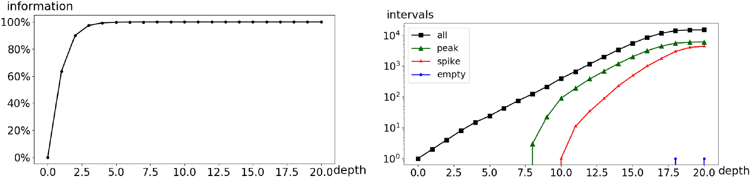

Figure 25.

LabWeb.

The values of the in-degrees are integers, which is correctly retrieved by the TMH method, with a truncation gap of 1. The 1^st obtained interpretable histogram, presented in Fig. 25b, contains 15,034 intervals. The histogram shows a clear decreasing power law behavior, with most of the nodes having a very small in-degree, and very few nodes having huge in-degrees. The first interval contains about 230 million nodes with a in-degree of 1. The last interval contains only 7 nodes (among 1 billion), for in-degrees spanning from 2 million to 20 million.

Although the general shape of the histogram is quite straightforward, it looks noisy for in-degrees between 1,000 and 1,000,000. A close inspection at some of these dense peaks shows that they are not pure noise: they actually reveal some surprising patterns. For example, there is one interval that contains 59 nodes with 297,690 or 297,691 in-degrees. It is surrounded by two intervals that are about one thousand times less dense: one with 14 nodes spanning over 2000 in-degrees values and another with 152 nodes spanning over 15,000 in-degrees values. Having such a concentration of node with almost exactly the same huge in-degree might be the signature of a Web farm.

Applying the methodology introduced in Section 7.3 allows to get a simplified summary of the in-degrees distribution and to capture its global shape. The indicators displayed in Fig. 24 suggest to coarsen the histogram from its initial granularity depth 20 down to 7, which is a considerable coarsening albeit with minimal loss of information. The simplified histogram, shown in Fig. 25c, consists of 75 intervals chosen among only 93 floating-point bins. It has a smooth decreasing power-law shape on seven orders of magnitude for the in-degrees and 15 orders of magnitude for the densities. The density estimation is accurate enough to distinguish two regimes for the power law, before and after around 10,000 in-degrees. It should be noted that these results are visually consistent with the frequency plot and Fibonacci binning provided with the data set (cf. Fig. 25a), both for the noisy patterns for in-degrees above 1,000 and for the overall shape of the distribution.

8.7 New York Times Annotated Corpus

The New York Times Annotated Corpus (NYTAC)7 contains over 1.8 million articles written and published by the New York Times between January 1, 1987 and June 19, 2007. Texts can be decomposed into sets of tokens, where tokens can be words, letters or even bytes, or their sequences named n-grams: n-grams of words, letters or bytes. In this section, we study the decomposition of the articles of the NYTAC into n-grams of bytes. There are about 166,000 distinct 3-grams in the corpus and their total number of occurrences is about 6.2 billion. Let us call the popularity of a 3-gram its number of occurrences in the corpus. A popular 3-gram has a large number of occurrences, while a noteless one has a small number of occurrences.8 We apply the G-Enum-fp method to summarize the density of this popularity variable for the 3-grams in the NYTAC. The popularity is an integer variable, which is recovered by the TMH method using a truncation gap of 1. The resulting histogram has 73 intervals and is directly interpretable, with a very smooth shape, as shown in Fig. 26a.

Figure 26.

New York Times Annotated Corpus: Popularity of n-grams.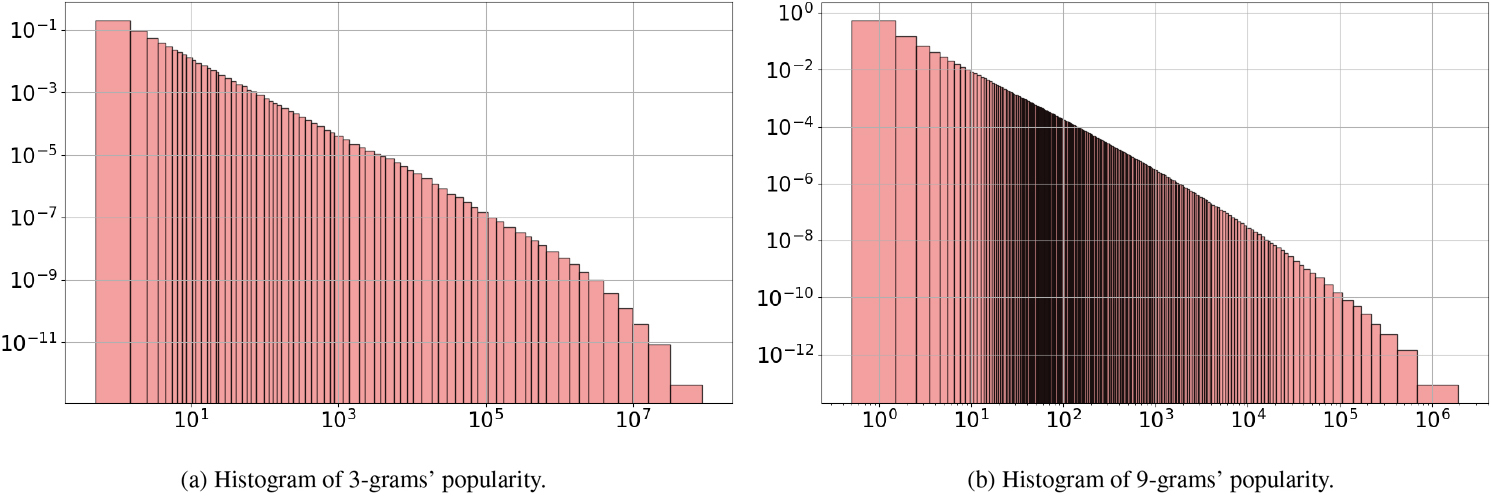

We evaluated the popularity of all n-grams of bytes, from 1-grams to 9-grams. We report the results for the 9-grams, which are the most numerous, with about 254 million distinct 9-grams in the corpus. The noteless 9-grams are very frequent, with over 134 million 9-grams having a popularity of 1. And the popular 9-grams are rare, the most popular “for the” having a popularity of around 1.9 million. The resulting histogram displayed in Fig. 26b is very accurate, with 230 intervals and a density spanning over 12 orders of magnitude. The length of the 65 first intervals is 1 while that of the last interval is greater than 1.2 million. This last interval contains the 27 most popular 9-grams, that behave as outliers in this histogram.

The histograms build for each kind the n-grams provide a smooth and accurate estimation of the underlying probability density function of the popularity of the n-grams. Although the data set combines several challenges, with integer data in addition to heavy-tailed distribution and large size, the retrieved histograms do not suffer from com-shaped or noisy patterns such as those displayed in Fig. 15. They are remarkably smooth and parsimonious, which make them easy to analyze and interpret. The shape of the density function given by the histograms is very similar for each kind of n-grams. It is almost a straight line, especially for the noteless n-grams, but is still concave, especially for the popular n-grams.

Figure 27.

New York Times Annotated Corpus: Zipf curves of 3-grams.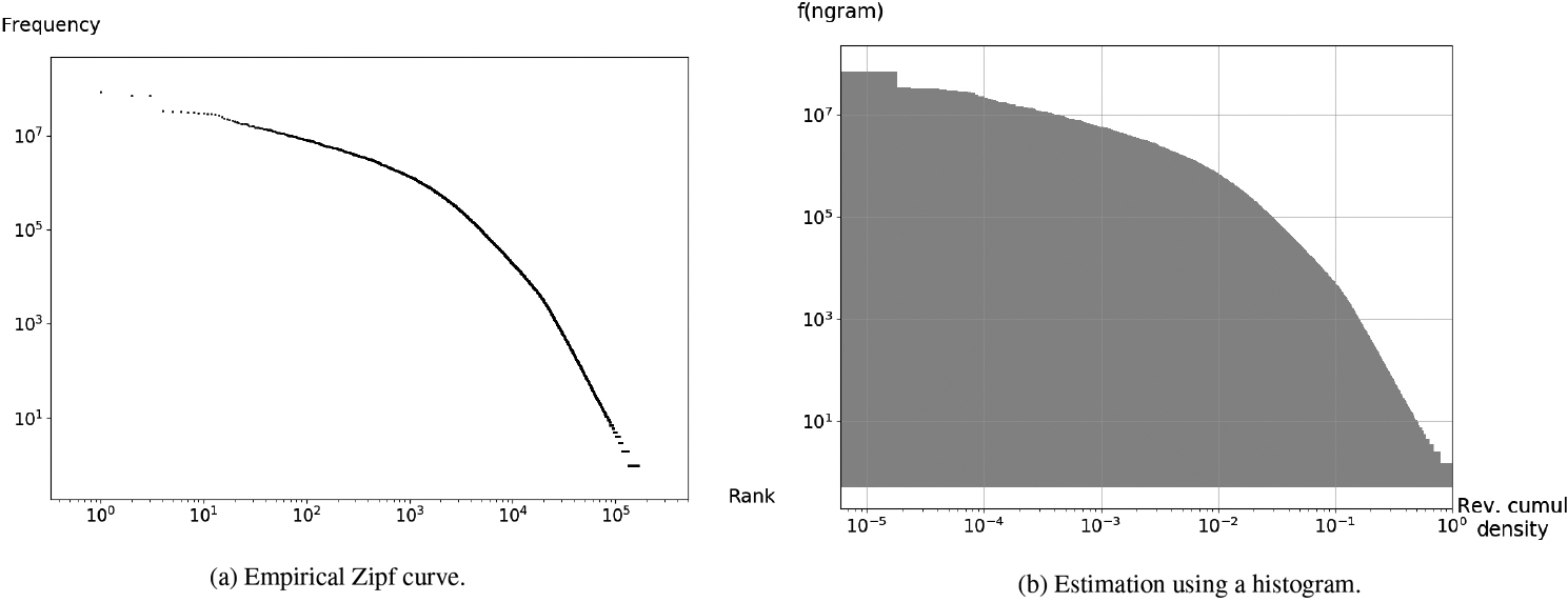

The frequency of tokens in text corpora has been widely studies in the literature. The Zipf’s law [26] for word tokens in a corpus states that if $f$ is the frequency of a word in the corpus and $r$ is the rank of a word by decreasing frequency, then $f=k/r$ where $k$ is a constant for the corpus. When $f$ is drawn in relation to $r$ using a $\log\times\log$ graph, which is called a Zipf curve, a straight line is obtained with a slope of $-1$ . To take into account deviations from this behavior, several modifications of the law have been proposed, in particular the one derived theoretically in [27], $f=\frac{k}{(r+\alpha)^{\beta}}$ where $\alpha$ and $\beta$ are constants for the analyzed corpus.

The Zipf curve for 3-grams in the NYTAC is drawn in Fig. 27a. Except for the least frequent 3-gram on the right side of the curve, the shape of the curve is clearly concave, far from a straight line. We now focus on the relationship between the Zipf curve for 3-grams in Fig. 27a and the probability density function of the popularity of 3-grams in Fig. 26a. Let $w_{i},1\leqslant i\leqslant n$ be a 3-grams, $f(w_{i})$ its frequency in the corpus, and $r(w_{i})$ its rank by decreasing frequency. The Zipf curve plots $r(w_{i})$ versus $f(w_{i})$ using a $\log\times\log$ scale. Let us now focus on the complementary cumulative distribution function (ccdf) of the popularity of 3-grams, that is

$\displaystyle\bar{F}_{X}(x)=P(X>x)$ (5)

where $X$ is the popularity variable, which is estimated using the frequency of the 3-grams. The empirical ccdf is computed from the data entries in the sample according to

$\displaystyle\hat{F}_{X}(x)=\frac{\text{number of 3-grams in the corpus with % popularity above x}}{n},$ (6) $\displaystyle=\frac{1}{n}\sum_{i=1}^{n}{{1}_{(f(w_{i})>x)}},$ (7)

where ${1}_{(f(w_{i})>x)}$ is 1 if $f(w_{i})>x$ and 0 otherwise. When 3-grams are sorted by decreasing frequencies, we have

$\displaystyle\hat{F}_{X}(f(w_{i}))=\frac{1}{n}r(w_{i}).$ (8)

This demonstrates that the Zipf curve is none other than the empirical ccdf of the popularity drawn using a $\log\times\log$ scale with the two axes inverted [28]. As the histogram displayed in Fig. 26a represents an estimate of the popularity distribution function of the 3-grams, we exploit it to get an estimate of the ccdf and obtain the graph displayed in Fig. 27b, based on 73 intervals instead of 166,000 points in the Zipf curve of Fig. 27a. This shows that the histograms obtained using the G-Enum-fp method provide a very accurate summary of the Zipf curve, much easier to study given their parsimony. It opens new research avenues for the study of the word frequency distribution, either directly using the probability distribution or its cumulative variants.9

9. Conclusion

In line with our goal of exploratory analysis of large scale real-world data sets, we chose the G-Enum histogram method [6] as our starting point because it is automatic, scalable, parsimonious and achieves state-of-the art accuracy in density estimation. The G-Enum method builds irregular histograms with intervals of variable lengths, based on a modeling space consisting of equal-width elementary bins. This makes sense for a piecewise-constant density estimator for distributions with real values in $\mathbb{R}$ . Although it works well in many cases, this method cannot cope with distant outliers or heavy-tailed distributions. When the number of equal-width elementary bins required to cover the entire value domain increases to its limits, the elementary bins become over-lengthy to properly approximate the dense density regions of the underlying distributions.

In this paper, we have suggested to extend the G-Enum method, by replacing its equal-width elementary bins by floating-point elementary bins that exploit the floating-point representation of real numbers on computers. This alternative representation space enables to treat any data set that can be represented on a computer, rather than data sets with values in $\mathbb{R}$ . The new method, named G-Enum-fp, keeps most of the features of the G-Enum method: the modeling space (only the definition of the elementary bins has changed), the evaluation criterion and the optimization heuristics. This allows to inherit from the appealing properties of the G-Enum method: parameter-less, robustness, accuracy, parsimony and scalability. Extensive experiments have been conducted to analyze the impact of this new representation space using various artificial distributions. The results show indistinguishable performance in the case of standard regular distributions. On the other hand, in the case of outliers or heavy-tailed distribution, the G-Enum-fp method brings considerable improvements, as it can accurately approximate the underlying distributions regardless of their shape and scale.

However, these very promising results collapsed during the first experiments with real data. The problem is not the limited precision of the computer representation of real numbers. As shown by artificial experiments with known distributions, the precision of the 15-digit decimal mantissa is clearly sufficient, even in the case of very large data sets. The problem is that real-world data sets involve a digitization process, with many potential issues such as for example, inherently integer data, biased data collection, limited recording accuracy, data transformation, rounding or truncation errors. As the size of the data sets increases, the digitized structure of the data may dominate the statistical structure of the original data, and accurate histograms retrieve the dominant structure, which may be of little interest for exploratory analysis. Abandoning the objective of fully automated histograms for exploratory analysis, we have proposed heuristics to process truncated data and eliminate singularities, as well as a methodology to facilitate the task of recovering the statistical structure of the data beyond their digitization structure. Extensive experiments on large scale real-world data sets show the effectiveness of the approach.

The first immediate objective of future work is to apply the methodology proposed in this paper to discover new insights in areas where histograms could not be easily applied previously. Another research direction includes extensions of the G-Enum-fp method to the processing of huge data stores or fast data streams. Finally, it is noteworthy that one of the most striking surprises in this article is the strong interweaving of digitization and statistical structures in large real-world data sets. This implies that accurate methods can sometimes produce results without much interest. As the current trend in supervised classification is to apply methods with numerous parameters on very large data sets, one can cautiously consider the excellent accuracy of the predictions obtained. Analyzing this potential issue appears to be a promising direction for research.

Footnotes

User parameters (e.g. $\epsilon$ ) have to be adjusted by the data analyst, model parameters belong to the modeling space and are inferred automatically by optimizing a criterion, technical parameters are internal constants, used for example as upper-bounds of model parameters (e.g. $E=10^{9}$ , with $1\leqslant G\leqslant E$ ).

https://astrogeology.usgs.gov/search/map/Moon/Research/Craters/GoranSalamuniccar_MoonCraters.

https://astrogeology.usgs.gov/search/map/Moon/Research/Craters/lunar_crater_database_robbins_2018.

https://www.datastro.eu/explore/dataset/hyg-stellar-database/information/.

For privacy reasons, this data set is not publicly available.

Available at http://law.di.unimi.it/webdata/eu-2015/ with some visualization plots.

Available from the Linguistic Data Consortium (LDC) at https://catalog.ldc.upenn.edu/LDC2008T19.

This notion of popularity for 3-grams has been introduced to avoid confusing comments such as “frequent words are rather infrequent” or “rare words are very frequent”.

The normalized word frequency $f(w_{i})/\sum_{j}{f(w_{j})}$ could also be used to obtain less corpus-dependent information.

Appendix

G-Enum-fp histogram method

In the Section 4, we have exploited the floating-point representation of real values to introduce an alternative definition of the elementary bins used as building blocks for a new histogram method called G-Enum-fp. We first summarize the principles of this new method, then detail its specific components.

Properties of G-Enum-fp method

In this section, we further analyze the G-Enum-fp criterion and investigate on some of its properties.

Experiments with common artificial data sets

In this appendix, we evaluate the G-Enum-fp method in the case of common artificial data sets, using the uniform, normal and a mixture of normal distributions. The evaluation protocol is that of Section 6.1.

References

Rissanen

Speed

T.P.

and Yu

, Density estimation by stochastic complexity, IEEE Transactions on Information Theory 38(2) (1992), 315–323.

Kontkanen

and MyllymÃ¤ki

, MDL Histogram Density Estimation, in: Proceedings of the Eleventh International Conference on Artificial Intelligence and Statistics Meila

and Shen

, eds, Proceedings of Machine Learning Research, Vol. 2, PMLR, 2007, pp. 219–226.

Davies

P.L.

and Kovac

, Densities, spectral densities and modality, Ann. Statist. 32(3) (2004), 1093–1136. doi: 10.1214/009053604000000364.

Rozenholc

Mildenberger

and Gather

, Combining regular and irregular histograms by penalized likelihood, Computational Statistics and Data Analysis 54(12) (2010), 3313–3323. doi: 10.1016/j.csda.2010.04.021. http://www.sciencedirect.com/science/article/pii/S0167947310001660.

Scargle

J.D.

Norris

J.P.

Jackson

and Chiang

, Studies in astronomical time series analysis. vi. bayesian block representations, The Astrophysical Journal 764(2) (2013), 167. doi: 10.1088/0004-637x/764/2/167. http://dx.doi.org/10.1088/0004-637X/764/2/167.

Zelaya Mendizábal

Boullé

and Rossi

, Fast and fully-automated histograms for large-scale data sets, Computational Statistics & Data Analysis 180 (2023), 107668. doi: 10.1016/j.csda.2022.107668. https://www-sciencedirect-com-443.web.bisu.edu.cn/science/article/pii/S0167947322002481.

Rissanen

, A universal prior for integers and estimation by minimum description length, Ann. Statist. 11(2) (1983), 416–431. doi: 10.1214/aos/1176346150.

Boullé

Clérot

and Hue

, Revisiting enumerative two-part crude MDL for Bernoulli and multinomial distributions (Extended version), arXiv 1608.05522, 2016.

Davies

Gather

Nordman

and Weinert

, A comparison of automatic histogram constructions, ESAIM: Probability and Statistics 13 (2009), 181–19.

10.

Freedman

and Diaconis

, On the histogram as a density estimator: L2 theory, Zeitschrift für Wahrscheinlichkeitstheorie und Verwandte Gebiete 57(4) (1981), 453–476. doi: 10.1007/BF01025868.

11.

Hodge

and Austin

, A survey of outlier detection methodologies, Artificial Intelligence Review 22 (2004), 85–126.

12.

Zhang

, Advancements of outlier detection: A survey, ICST Transactions on Scalable Information Systems 13(1) (2013), 1–26.

13.

Gebski

and Wong

R.K.

, An efficient histogram method for outlier detection, in: Advances in Databases: Concepts, Systems and Applications: 12th International Conference on Database Systems for Advanced Applications, DASFAA 2007, Bangkok, Thailand, April 9–12, 2007. Proceedings 12, Springer, 2007, pp. 176–187.

14.

Boullé

, Two-level histograms for dealing with outliers and heavy tail distributions, arXiv 2306.05786, 2023.

15.

IEEE, IEEE Standard for Binary Floating-Point Arithmetic, ANSI/IEEE Std 754-1985, 1985, 1–20. doi: 10.1109/IEEESTD.1985.82928.

16.

Dua

and Graff

, UCI Machine Learning Repository, 2017. http://archive.ics.uci.edu/ml.

17.

Knuth

K.H.

Castle

J.P.

and Wheeler

K.R.

, Identifying excessively rounded or truncated data, in: Compstat 2006 – Proceedings in Computational Statistics Rizzi

and Vichi

, eds, Springer, 2006, pp. 313–323.

18.

Azzalini

and Bowman

A.W.

, A look at some data on the old faithful geyser, Journal of the Royal Statistical Society. Series C (Applied Statistics) 39(3) (1990), 357–365.

19.

Marx

Yang

and van Leeuwen

, Estimating Conditional Mutual Information for Discrete-Continuous Mixtures using Multi-Dimensional Adaptive Histograms, in: Proceedings of the 2021 SIAM International Conference on Data Mining, SDM 2021, Virtual Event, April 29–May 1, 2021 Demeniconi

and Davidson

, eds, SIAM, 2021, pp. 387–395.

20.

Tukey

J.W.

, Exploratory Data Analysis, Addison-Wesley, 1977.

21.

Salamunićcar

Lončarić

and Mazarico

, LU60645GT and MA132843GT catalogues of Lunar and Martian impact craters developed using a Crater Shape-based interpolation crater detection algorithm for topography data, Planetary and Space Science 60(1) (2012), 236–247.

22.

Robbins

S.J.

, A New Global Database of Lunar Impact Craters > 1–2 km: 1. Crater Locations and Sizes, Comparisons With Published Databases, and Global Analysis, Journal of Geophysical Research (Planets) 124(4) (2019), 871–892. doi: 10.1029/2018JE005592.

23.

Wang

and Zhou

J.-L.

, Determining proportions of lunar crater populations by fitting crater size distribution, Research in Astronomy and Astrophysics 16(12) (2016), 185.

24.

Boldi

and Vigna

, The WebGraph Framework I: Compression Techniques, in: Proc. of the Thirteenth International World Wide Web Conference (WWW 2004), ACM Press, 2004, pp. 595–601.

25.

Boldi

Rosa

Santini

and Vigna

, Layered Label Propagation: A MultiResolution Coordinate-Free Ordering for Compressing Social Networks, in: Proceedings of the 20th international conference on World Wide Web Srinivasan

Ramamritham

Kumar

Ravindra

M.P.

Bertino

and Kumar

, eds, ACM Press, 2011, pp. 587–596.

26.

Zipf

G.K.

, Human Behaviour and the Principle of Least Effort, Addison-Wesley, 1949.

27.

Mandelbrot

, An Information Theory of the Statistical Structure of Language, in: Communication Theory, Academic Press, 1953, pp. 486–502.

28.

Newman

, Power laws, Pareto distributions and Zipf’s law, Contemporary Physics 46(5) (2005), 323–351. doi: 10.1080/00107510500052444.

29.

Shannon

C.E.

, A mathematical theory of communication, Technical Report, 27, Bell systems technical journal, 1948.

30.

Grünwald

P.D.

, The minimum description length principle, Adaptive computation and machine learning, MIT Press, 2007.

31.

Kontkanen

, Computationally efficient methods for MDL-optimal density estimation and data clustering, Department of Computer Science, series of publications A, report, 2009-11, University of Helsinki, 2009.

32.

Mononen

and Myllymäki

, Computing the multinomial stochastic complexity in sub-linear time, in: Proceedings of the 4th European Workshop on Probabilistic Graphical Models (PGM-08), September 17–19, 2008, Hirtshals, Denmark, 2008, pp. 209–216, Volume: Proceeding volume.

33.

Rissanen

, Fisher information and stochastic complexity, IEEE Transactions on Information Theory 42(1) (1996), 40–47.

34.

Szpankowski

, On asymptotics of certain recurrences arising in universal coding, Problems of Information Transmission 34(2) (1998), 142–146.

35.

Brooks

Lee

E.A.

Liu

Neuendorffer

Zhao

and Zheng

, Heterogeneous Concurrent Modeling and Design in Java, Technical Report, Technical Memorandum UCB/ERL M04/27, University of California, 2004. http://ptolemy.eecs.berkeley.edu/publications/papers/04/ptIIDesignIntro/.

36.

Boullé

, Recherche d’une représentation des données efficace pour la fouille des grandes bases de données, PhD thesis, Ecole Nationale Supérieure des Télécommunications, 2007.

37.

Boullé

, MODL: a Bayes optimal discretization method for continuous attributes, Machine Learning 65(1) (2006), 131–165.

38.

Rissanen

J.J.

, Fisher information and stochastic complexity, IEEE Transactions on Information Theory 42(1) (1996), 40–47. doi: 10.1109/18.481776.

39.

Dua

and Graff

, UCI Machine Learning Repository, 2017. http://archive.ics.uci.edu/ml.

40.

Kontkanen

Buntine

W.L.

Myllymäki

Rissanen

and Tirri

, Efficient Computing of Stochastic Complexity, in: Proceedings of the Ninth International Workshop on Artificial Intelligence and Statistics, AISTATS 2003, Key West, Florida, USA, January 3–6, 2003, 2003. http://research.microsoft.com/en-us/um/cambridge/events/aistats2003/proceedings/172.pdf.

41.

Rissanen

, Modeling by shortest data description, Automatica 14 (1978), 465–471.

42.

Davies

and Kovac

, ftnonpar: Features and Strings for Nonparametric Regression, 2012, R package version 0.1-88. https://CRAN.R-project.org/package=ftnonpar.

43.

Mildenberger

Rozenholc

and Zasada

, histogram: Construction of Regular and Irregular Histograms with Different Options for Automatic Choice of Bins, 2019, R package version 0.0-25. https://CRAN.R-project.org/package=histogram.

44.

Harris

C.R.

Millman

K.J.

van der Walt

S.J.

Gommers

Virtanen

Cournapeau

Wieser

Taylor

Berg

Smith

N.J.

Kern

Picus

Hoyer

van Kerkwijk

M.H.

Brett

Haldane

del Río

J.F.

Wiebe

Peterson

Gérard-Marchant

Sheppard

Reddy

Weckesser

Abbasi

Gohlke

and Oliphant

T.E.

, Array programming with NumPy, Nature 585(7825) (2020), 357–362. doi: 10.1038/s41586-020-2649-2.

45.

Astropy Collaboration Price-Whelan

A.M.

Lim

P.L.

Earl

Starkman

Bradley

Shupe

D.L.

Patil

A.A.

Corrales

Brasseur

C.E.

Nöthe

Donath

Tollerud

Morris

B.M.

Ginsburg

Vaher

Weaver

B.A.

Tocknell

Jamieson

van Kerkwijk

M.H.

Robitaille

T.P.

Merry

Bachetti

G"unther

H.M.

Aldcroft

T.L.

Alvarado-Montes

J.A.

Archibald

A.M.

B’odi

Bapat

Barentsen

Baz’an

Biswas

Boquien

Burke

D.J.

Cara

Conroy

K.E.

Conseil

Craig

M.W.

Cross

R.M.

Cruz

K.L.

D’Eugenio

Dencheva

Devillepoix

H.A.R.

Dietrich

J.P.

Eigenbrot

A.D.

Erben

Ferreira

Foreman-Mackey

Fox

Freij

Garg

Geda

Glattly

Gondhalekar

Gordon

K.D.

Grant

Greenfield

Groener

A.M.

Guest

Gurovich

Handberg

Hart

Hatfield-Dodds

Homeier

Hosseinzadeh

Jenness

Jones

C.K.

Joseph

Kalmbach

J.B.

Karamehmetoglu

Kaluszy’nski

Kelley

M.S.P.

Kern

Kerzendorf

W.E.

Koch

E.W.

Kulumani

Lee

MacBride

Maljaars

J.M.

Muna

Murphy

N.A.

Norman

O’Steen

Oman

K.A.

Pacifici

Pascual

Pascual-Granado

Patil

R.R.

Perren

G.I.

Pickering

T.E.

Rastogi

Roulston

B.R.

Ryan

D.F.

Rykoff

E.S.

Sabater

Sakurikar

Salgado

Sanghi

Saunders

Savchenko

Schwardt

Seifert-Eckert

Shih

A.Y.

Jain

A.S.

Shukla

Sick

Simpson

Singanamalla

Singer

L.P.

Singhal

Sinha

SipHocz

B.M.

Spitler

L.R.

Stansby

Streicher

Sumak

Swinbank

J.D.

Taranu

D.S.

Tewary

Tremblay

G.R.

Val-Borro

M.d.

Van Kooten

S.J.

Vasovi’c

Verma

de Miranda Cardoso

J.V.

Williams

P.K.G.

Wilson

T.J.

Winkel

Wood-Vasey

W.M.

Xue

Yoachim

Zhang

Zonca

and Astropy Project Contributors, The Astropy Project: Sustaining and Growing a Community-oriented Open-source Project and the Latest Major Release (v5.0) of the Core Package, apj 935(2) (2022), 167. doi: 10.3847/1538-4357/ac7c74.

46.

Boullé

, Two-level histograms for dealing with outliers and heavy tail distributions, 2023.

Floating-point histograms for exploratory analysis of large scale real-world data sets

Abstract

Keywords

1. Introduction

2. G-Enum method: Summary

2.1 Problem formulation

2.2 Granularity and choice of ϵ

2.3 Enum and G-Enum criteria for histogram models

Table 1 Term comparison of the Enum and G-Enum criteria

2.5 Experimental results

3. Limits of histogram methods w.r.t. outliers

3.1 Illustative exemple

3.2 Possible solutions to push these limits

3.2.1 Use of long integers

3.2.2 Removing outliers

3.2.3 Extension to hierarchical histogram models

3.2.4 Bi-level heuristic for histograms

4. Floating-point bins for histograms

4.1 Floating-point representation

Impact on histograms

4.2 Floating-point bins

Example with one single main bin

Example with multiple main bins

5.1 Principle

5.2 Specification of domain bounds

5.3 Choice of the central bin

5.4 G-Enum-fp criterion

Table 2 G-Enum-fp criterion

6.1 Evaluation protocol

Metrics

Histogram methods

Data sets

6.2 Normal distribution with an outlier

7.1 Applying histograms to real-world data sets

7.2.1 Dealing with integer data

7.2.2 Dealing with truncated data

Detection of truncated data

Calculation of the truncation gap

Construction of a histogram adapted to truncated data

7.3.1 Series of histograms

7.3.2 Indicators per histogram

7.4.1 Old faithful geyser

Discussion

8.1 Evaluation protocol

Footnotes

Appendix

G-Enum-fp histogram method

Properties of G-Enum-fp method

Experiments with common artificial data sets

References

2.2 Granularity and choice of $\epsilon$

Table 1
Term comparison of the Enum and G-Enum criteria

Table 2
G-Enum-fp criterion