Machine learning based car accident risk prediction for usage-based insurance

Abstract

The Usage-Based Insurance paradigm, which is receiving a lot of attention in recent years, envisages computing the car policy premium based on accident risk probability, evaluated observing the past driving history and habits. However, Usage-Based Insurance strategies are usually based on simple empirical decision rules built on travelled distance. The development of intelligent systems for smart risk prediction using the stored overall driving behaviour, without the need of other insurance or socio-demographic information, is still an open challenge. This work aims at exploring a comprehensive machine learning-based approach solely based on driving-related data of private vehicles. The anonymized dataset employed in this study is provided by the telematics company UnipolTech, and contains space/time densely measured data related to trips of almost 100000 vehicles uniformly spread on the Italian territory, recorded every 2 km by on-board telematics fix devices (black boxes), from February 2018 to February 2020. An innovative feature engineering process is proposed, with the aim of uncovering novel informative quantities able to disclose complex aspects of driving behaviour. Recent and powerful learning techniques are explored to develop advanced predictive models, able to provide a reliable accident probability for each vehicle, automatically managing the critical imbalance intrinsically peculiar this kind of datasets.

Keywords

Mobility data usage-based insurance machine learning driving behavior accident risk prediction

1. Introduction

Usage-Based Insurance (UBI) for road vehicles is a new innovative concept that has quite recently started to be commercialized around the world. The main idea is that instead of a fixed price, drivers pay a premium based on their travel and driving behaviour. For UBI, insurers employ vehicular sensor data in the determination of individual accident risk. Essentially, this enables insurance tariffs that more precisely reflect the actual risk exposure of insured vehicles and are adaptive over time, thereby yielding risk-minimizing incentives for policyholders. In consequence, information asymmetry between insurers and policyholders is reduced but also a significant improvement of traffic safety arises, [1], helping to decrease the approximately 1.3 million fatalities occurring each year as a result of road traffic crashes, [2].

Yet, even if UBI plans are adopted on a large scale globally, they commonly relate the risk of accident to data that are definitely too basic and naive. This might be attributed to data shortage to validate advanced procedures and to methodological deficiencies that persist among researchers and insurance practitioners with respect to the nature and structure of risk models estimated from telematics data, which nevertheless must always take into account the strong privacy concerns consumers hold against sharing data from their cars.

This work aims to address this issue and relies on a huge dataset of vehicles’ trips collected over two years throughout the entire territory in Italy, a pioneering European UBI insurance market, by the second major Italian insurance group, Unipol Group. Based on GPS-derived trajectory segments of almost 100000 anonymized private cars, various metrics of vehicle exposure are introduced and used to estimate supervised Machine Learning models in order to exploit the predictive information contained in the driving data with the most innovative data analytics methods, generating a more accurate forecast of the probability of claims. In this paper we will address and answer the issues related to how to define and extract the best risk-relevant features from the source dataset, how to deal with the complexity of a prediction problem with a strong intrinsic imbalance between the negative (no accident) and positive (one or more accident) class in the training data, how to select the most suited and powerful Machine Learning model in order to uncover the most predictive power of the telematics data and, ultimately, how to validate the model behavior and compare it to literature results. Concerning the first issue of feature engineering, the proposed solutions include static/aggregated or dynamic/time-series based features based on driving pattern primary variables like mileage, average and instantaneous speed, driving time and number of trips. Since risky behaviours are considerably less than safe ones, the data output class label is severely unbalanced and the problem particularly complex, so many techniques are explored and compared in order to best tackle this challenge. With regard to the model issues, an innovative Gradient Boosting approach is adopted, and its predictive power compared through quantitative metrics on unseen data, both using static and dynamic features. For completeness, we wish to recall here that the potential of big data coming from black boxes to extract useful information for insurance strategy planning has also been shown in [3, 4, 5] considering different decision making problems.

As a final note, our primary focus will be on predicting the occurrence of accidents, irrespective of their diverse nature. While acknowledging the existence of various accident types, our emphasis lies in forecasting the probability of accidents within the insurance industry’s current operational context. This predictive capability holds transformative potential, offering benefits to both customers – possibly leading to reduced premiums for cautious driving – and insurance companies, which can promote safer driving practices while efficiently allocating resources for high-risk scenarios. Additionally, it’s important to acknowledge that distinguishing between different accident types would be impractical due to limited data availability for each specific crash category.

The paper is organized as follows. In Section 2, the state of the art of UBI is illustrated and the dataset is described. Section 3 illustrates the rationale to construct the set of input features from the raw trips data. Section 4. Sections 5 and 6 describe how Machine Learning can be applied to predict the future accident probability and illustrates the experimental results. The paper is ended by some concluding remarks.

2. Background and problem setting

The UBI global market is estimated at $$ 33.1$ billion in 2020 and projected to reach $$ 110.2$ billion by 2027. This growth pushes insurance companies to always keep up with the latest UBI technologies and to make the best of the huge amount of the measured driving data. Furthermore, also the research world is actively involved in the UBI field, mainly as subject of academic study in the data analytics and, most recently, machine learning fields.

Data gathering for UBI can be performed through different sources, influencing on one side the structural integration and dependency on the vehicle, and on the other the measurements continuity in space and precision. Through the CAN bus reached through a dongle connected to the exposed On-Board Diagnostic (OBD) interface. This kind of device is not expensive and could potentially be self-fitted by the user himself and hence usually chosen by car manufacturers; however, this solution is highly vehicle-dependent. On the opposite side, through a smartphone: this kind of solution is the most recent one and can be used either as a stand-alone device or can be linked to the information system of the vehicle, but definitely suffers from the difficulty to maintain a stable position in order to provide accurate data, in addition to the issue that smartphones are not always active. Lastly, data can be collected through black boxes, professional devices installed on vehicle battery; they require some effort to be installed, but they are firmly fasten on the vehicle and able to provide a continuous, reliable and robust stream of data. The employment of vehicle sensors enables the introduction of new information related to real driving patterns: each insurer has different perspective on the weight to give to each measured quantity, but generally it has been proven that the most important are driven mileage, driven time and accelerations, [6]. Many researches on UBI based on driving behaviour integrate their models with variables like vehicle type or or customer or vehicle age or residence town, [7], in addition to some complex variables like acceleration, deceleration and braking intensities or sudden turns.

This work is based on the UnipolTech telematics data. UnipolTech is part of Unipol Group, the second largest Italian insurance company and a pioneer of telematics in car insurance market, with 4.5 millions black boxes installed on private vehicles. Driving data originate from GPS sensors embedded in the black boxes of 94268 private vehicles registered all over Italy, gathered during the period from February 2018 to February 2020. These black boxes are attached to the car battery and always powered so that no interruption in the information stream can happen. The vehicles driving history is mapped in the trips dataset, which is composed of about 426Mio entries. A trip is generated aggregating the so called raw events, which are recorded by car GPS sensors at 1 Hz and roughly every 2 km sent and stored in the company’s servers for later processing. An event is represented by a location in space and time, and is later processed into a more compact format, which is that of a trip. Each trip is characterized by its spatial and temporal information (i.e. timestamps and coordinates of the route starting and end points), together with additional information regarding the total distance and duration of the trip, the average driving speed during the trip computed as trip distance divided by trip driving time, the average instant speed i.e. the average driving speed recorded by black boxes every 2 km, and the number of accidents occurred during the trip.

This trips dataset is the starting point for the following feature engineering process and learning algorithms. It is worth mentioning that this work is focused on the building of UBI learning models solely based on GPS driving pattern information, not including neither static information nor additional dynamic information, like acceleration/deceleration events or braking and sudden turns indicators. The inclusion of these kind of features could probably improve the risk probability prediction accuracy, but our aim is to rely just on the cheap, immediate GPS measurements of the black boxes.

3. Static and dynamic features engineering for measuring driving behavior

Trips associated to each vehicle cannot be used as they are to train learning models and their characteristics have to be shrunk properly into suitable and meaningful numerical features. In any case, before outlining the process of creating these compact features linked to the behavior of each car, the data sizes before and after pre-processing (elimination of null or inconsistent samples and outliers) are shown in Table 1.

Table 1
Dataset overview before and after pre-processing.

Geographic region Number of analysed vehicles Number of trips $[\times 10^{6}]$

Italy Original 94268 426

Preprocessed 88120 395

Geographic region		Number of analysed vehicles	Number of trips $[\times 10^{6}]$
Italy	Original	94268	426
	Preprocessed	88120	395

The paper explores two ways of building this features dataset. The first one consists of generating static overall quantities comprehensively translating into space and time information each vehicle’s driving activity. The latter is a classical way of approaching features building in UBI problems, numerically representing the overall behavior of drivers over the geographical and temporal observation horizon.

The second, innovative way of building the features dataset has never bee explored before in this field and is based on the idea of not summing up the sequential trips information but exploiting their inter-day variability building up time-series (for example of driven distances, etc.). These time-series showcase also the dynamic variability of driving data, like for example correlations, and can capture much more complex aspects of driving behavior highlighted by its representation as an evolving time-series.

3.1 Static driving behavior features

Addressing the feature engineering task in accordance with the first, classical approach, some static features can be directly computed from the raw collection of trips for each vehicle and are the following:

First to last [days]: number of days between the first and the last recorded trip

Total mileage [km]

Average number of trips: total number of trips divided by first to last value

Total driving time [min]

Average speed [km/h]: sum of average speeds divided by first to last value

Average instant speed [km/h]: sum of instant speeds divided by first to last value

Active days [days]: number of days with recorded trips

Furthermore, some additional, meaningful metric can be derived, on top of the above listed primary ones, through further manipulations or relying on the intersection of trips’ GPS track with road maps associating each latitude/longitude point with a specific type of road – urban, extraurban, highway – and each instant speed measurement with the actual speed limit. Thereby, the following additional quantities are added:

Activity index: ratio between active days and first to last.

Average positive delta speed: sum of the differences between average speed and speed limit for the specific, prevalent road type, if the difference is greater than 10 km/h, 0 otherwise.

Number of speed limit infractions: Number of times the vehicle exceeds the specific road speed limit, by at least 10 km/h.

Exploiting the information on the start and end time and spatial coordinates of each trip, the aforementioned features can also be valuably disaggregated according to the different time slots during the day: Early morning (0–6 a.m.), A.M. peak time (6–9 a.m.), Morning (9–12 a.m.), Afternoon (0–5 p.m.), P.M peak time: (5–8 p.m.), Night (8–12 p.m.), and to the three different road types: Urban, Extraurban, Highway.

Itemizing all the metrics with respect to various time slots and road types enables the definition of time of day/road more focused features, since most of the literature highlights the existence of periods of the day or type of roads where the accident rate is significantly higher. The result of this “classical” features extraction process is a set of mixed integer and real numbers (one for each vehicle) built taking into consideration the previously mentioned steps of features extraction. The overall, typological framework of the static features collection is:

3 Global Activity features: First to last, Active days, Activity

5 Global Driving Features: Total mileage, Total driving time, Average instant speed, Average speed, Average number of trips

18 “Road type” Specialized features: Mileage, Driving time, Average instant speed, Average speed, Average positive delta speed, Number of speed limit infractions

30 “Time slot” Specialized features: Mileage, Driving time, Average instant speed, Average speed, Average number of trips

108 “Time slot $+$ Road type” Twofold Specialized features: Mileage, Driving time, Average instant speed, Average speed, Average positive delta speed, Number of speed limit infractions

Figure 1.

Static features engineering schematic pipeline.

According to the schematic representation in Fig. 1, the accident risk prediction model will therefore be built on the basis of the dataset of the above mentioned 164 quantities for all the observed vehicles, where the output information is also known, i.e. the number of accidents occurring to the specific vehicle in the period of observation of the data.

3.2 Dynamic driving behavior features exploiting time-series

The classical static variables illustrated in Section 3.1 kind of squeeze the behavior of vehicles through sums and averages, possibly fragmented with respect of “when” and “where” the mileage or the duration of trips has been performed. However single trips from vehicles potentially contain new and more informative behavior patterns, represented by finer features able to uncover even remarkable changes in the driving style through both time and space. Vehicles drive independently from each other, so their number of trips can strongly vary and does not obviously follow a constant frequency.

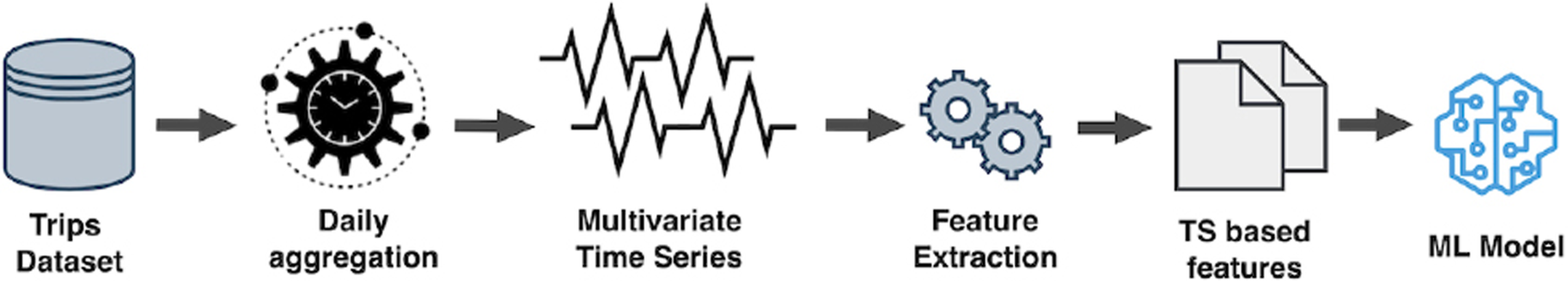
In order to properly model the evolution of driving behaviour through time and extract reliable time-dependent features, trips are first aggregated on a daily basis, since the “day” time unit seems a meaningful one and this time sampling is common to all the vehicles. This results in a time series of daily observations for each vehicle. The operational details on the construction and resolution of a generic time-series are as follows:

Trips belonging to the same day (0 a.m.–12 p.m.) and vehicle are aggregated together, meaning that all their values of mileage, duration, etc. are summed or averaged (for speeds) in order to form a single daily sample.

During the daily aggregation, also road types, time slots and combined variables are extracted for each day: in this way we don’t discard the useful hour and space disaggregations and each daily observation comprises the 164 variables presented in 3.1.

If a vehicle does not have any trip during a particular day, meaning that it didn’t drive, the daily sample is created nonetheless, setting all its features to 0. In this way we are able to fully represent the day-by-day evolution of behaviour and all the extracted sequences of days have the same length (roughly 730 days, that is, two years).

This process extracts, for each vehicle, a multivariate daily time series, which includes 164 univariate time series.

In a Machine Learning framework, there are mainly two approaches to extract features from multivariate time series: domain knowledge can be exploited to manually extract features which are able to represent time series’ fundamental aspects or the multivariate time series can be directly fed to a Deep Learning algorithm as they are, without any intermediate feature engineering process. For example, a neural network is automatically able to extract meaningful features, if properly trained in the right supervised or unsupervised learning framework. Nonetheless, often the generated metrics loose the concrete meaning of the original ones, and the insight into their real meaning might be difficult.

The approach utilized here is pioneering, as it enables the creation of a more interpretable feature set and subsequent predictive model. Initially, numerous primary metrics are extracted individually from each of the 164 time series for every vehicle. Subsequently, during a feature selection process, some metrics are filtered out to prevent excessive burden on the prediction task without sacrificing accuracy. This optimization is possible because many features lack relevance for our objectives. Additionally, it’s important to note that processing raw time series would demand significant computational time and necessitate the introduction of additional approximations, potentially compromising performance further. The first type of features that will be extracted are the most immediate and intuitive ones, which are only dependent on the absolute value of the time series points but not on their specific order in time, but they can still be able to describe relevant variability aspects:

Standard Deviation: gives an idea of the overall variability of the behaviour of a user during the two years;

Maximum Value;

Number of Samples Above the Mean: it is representative of the number of days in which the vehicle drove more than the mean mileage over two years;

Number of Samples Below the Mean.

A second set of features takes value strictly depending on the specific temporal order of time series points:

Complexity Estimate (CE): originally introduced as the basis for a Complexity-Invariant Distance measurement between time series [8], this metric is an estimate for time series complexity, since it captures peaks and valleys in the temporal sequence. A higher value of this metric means, in our context, that the vehicle is driven quite irregularly and he tends to behave quite differently from day to day.

The CE of a time series is computed as

C E (x) = \sqrt{\sum_{t = 0}^{T - 1} (x_{t} - x_{t + 1})^{2}}

(1)

where

x

is the considered time series,

T

is the length of the time series,

x_{t}

and

x_{t + 1}

are two generic consecutive time series points.

Spectral Centroid: The spectral centroid is the center of ‘gravity’ of the spectrum. It is calculated as the weighted mean of the frequencies present in the signal, determined using a Fourier transform, with their magnitudes as the weights. The Spectral Centroid feature has been mainly used as a measure of brightness of the sound [9].

In the present context of daily time series, there is not a real physical association to this feature, which is anyway developed since the FFT transformation could reveal, in the frequency domain, some patterns that in time domain just can’t be brought to light. The formula to compute the Spectral Centroid is

\begin{aligned} S C = \frac{\sum_{n = 0}^{N - 1} f (n) a (n)}{\sum_{n = 0}^{N - 1} a (n)} \end{aligned}

(2)

where

a (n)

represents the weighted frequency magnitude of bin number

n

, and

f (n)

represents the center frequency of that bin.

N

is the total number of FFT bins.

Autocorrelation Estimation with Lag 1: Autocorrelation of the time series at specified lags, using the following formula

\begin{aligned} R_{1} = \frac{1}{(T - 1) σ^{2}} \sum_{t = 1}^{T - 1} (x_{t} - μ) (x_{t + 1} - μ) \end{aligned}

(3)

where 1 is the lag,

T

is the length of the time series,

σ^{2}

is its variance and

μ

its mean. This features is developed since series from class 1 and class 0 might show, on average, different autocorrelation values, giving this feature a potentially important discrimination capability.

Mean Absolute Changes: The physical meaning of this feature is very similar to the Complexity Estimate (the main difference is that this is a mean measure of the irregularity), since it models the complexity of the sequence by computing how much, on average, the behaviour changes from one day to the subsequent:

\begin{aligned} MAC = \frac{1}{T} \sum_{t = 1}^{T - 1} | x_{t + 1} - x_{t} | \end{aligned}

(4)

C3 Statistics with Lag 1: This statistics has been proposed by Schreiber and Schmitz [10] as a feature with good discrimination probability, which measures the non-linearity of time series. The formula is the following

\begin{aligned} C 3_{1} = \frac{1}{T - 2} \sum_{t = 1}^{T - 2} x_{t + 2} \cdot x_{t + 1} \cdot x_{t} \end{aligned}

(5)

Figure 2.

Dynamic, time series based, features engineering schematic pipeline.

The extraction of the listed features for each time series of each vehicle allows the construction of a huge dynamic feature set that will be fed to a Machine Learning model to compute the risk probability, Fig. 2. As in the static dataset, the accident rate is known for every vehicle.

4. Accident probability prediction

In real UBI programs, insurance companies track the chosen set of driving-related variables and employ a custom decision process to evaluate the entity of the premium. The first step to build a UBI plan is to develop a decision process to map the input variables to a score to be assigned the insured vehicles, which represents the basis for the UBI premium integration. The traditional solutions involve using simple rule-based decisions, employing thresholds to distinguish between normal and dangerous driving behaviour [11]. The rules and thresholds are usually developed by experts in autonomous driving, driving simulation, behavioral risk assessment, and similar fields [12]. Other approaches consider instead a set of predefined templates developed by transportation experts, that describe different driving behaviours, ranging from safe to dangerous ones. Pattern matching algorithms are then used to assign the vehicles to the most similar template [13]. In recent years, some researchers have proposed Machine Learning approaches to tackle UBI, either from an Unsupervised Learning point of view, extracting insights from data, or from a supervised one, using Machine Learning models to capture the non-linear, causal relationships between driving behaviour and accident risk. This is still a relatively young field of study and most of the literature works do not properly illustrate and highlight the Machine Learning methodology itself but concentrate on the application and results [6, 14]. Furthermore, most of the times, literature results are based on data collected with simulations or with surveys and even when real data is employed, the information is poor and probably not able to reflect the real variable and accident distribution, [15]. This work focuses on Machine Learning approaches that for their structure, behavior and peculiarities best fit to the characteristics of the telematics dataset at hand, to the type of input features and to the requested performance.

4.1 The Machine Learning methodology

In recent years, some researchers have proposed intelligent and automatic Machine Learning approaches to tackle UBI issues, either in an Unsupervised Learning setting, extracting insights from data, or in a Supervised one, using Machine Learning models to capture the non-linear, causal relationships between driving behaviour and accident risk. In this paper, knowing the vehicles’ accidentality in the observation period, we face the challenge of determining a Supervised Learning solution able, once trained and tested, to map an new vehicle’s data and generate its crash probability with a satisfactory accurancy.

Each vehicle’s driving history data is provided together with the number of occurred crashes over the two years observaton period. We have condensed this target information into a binary label associated to each vehicle, in order to specify the presence or not of accidents during the entire observation period:

Safe vehicles (Class 0): that have no accidents in the observation period

Dangerous vehicles (Class 1): with one or more accidents in the observation period

The problem locates therefore itself within the family of Supervised Binary Classification Machine Learning tasks.

4.1.1 The class imbalance problem

Only 5% of vehicles fall into Class 1. The prevalence of safe behaviors over risky ones is a fundamental characteristic of accident risk prediction. This stems from the fact that only a small fraction of insured users experience accidents within a two-year observation period. This 5% can be regarded as the prior probability of being involved in a car crash. The issue of class imbalance presents two significant challenges. Firstly, a standard classifier would exhibit a strong bias towards the majority class, thereby struggling to assign appropriate significance to minority samples. Additionally, the conventional accuracy metric used to assess prediction performance would lead to the “accuracy paradox”. For instance, a dummy classifier that consistently predicts Class 0 for all samples would achieve 95% accuracy, yet it would fail to generalize effectively.

Many solutions have been proposed to solve the imbalance problem and they can be split into 3 main categories [16]:

Data Level techniques: they reduce the class imbalance acting on the dataset before training the classifier.

Algorithm Level techniques: they reduce the class imbalance by exploiting specific rationale to counteract the imbalance within the Machine Learning algorithm itself.

Cost Level techniques: they reduce the class imbalance by changing the cost function to be optimized within the Machine Learning algorithm itself.

The solution proposed in this paper consists of a Cost Level technique, exploiting a cost-sensitive version of the Gradient Boosting algorithm.

In order to solve the “accuracy paradox” and have a more robust evaluation method, a lot of different metrics have been implemented. The Area Under the Receiver Operating Characteristic (ROC) Curve is a 2-axis graph showing the performance of a binary classification model adopting different thresholds. The area under this curve indicates how good a classifier is at discriminating classes, regardless of the applied threshold. A value of 0.5 characterizes a classifier with no skills, while an AUC of 1 indicates a perfect classifier.

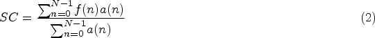
Alongside the ROC curve, another evaluation perspective is given by the Balanced Accuracy. This performance metric is defined as

\frac{1}{2} (\frac{T P}{T P + F N} + \frac{T N}{T N + F P})

where the first term in brackets is the True Positive Rate (TPR) and the second is called True Negative Rate (TNR). The Balanced Accuracy is therefore a balanced combination of these two indexes.

4.1.2 Cost-sensitive Gradient Boosting learning framework

The Gradient Boosting algorithm has proven to be one of the most successful Machine Learning models [17].

It is an implementation of the more general Boosting algorithm, which consists of the sequential training of multiple weak learners (the base employed model, often characterized by a strong bias and low variance). Each weak learner focuses where its predecessor failed, giving larger weights to previously bad predicted samples. In this way, the final model is usually able to perform enormously better than the single weak learners.

In the Gradient Boosting implementation, each base learner tries to correct the residual errors in the prediction made by the previous learners. Moreover, when used to solve a binary classification task, this algorithm can output a probability-like prediction, giving richer information than the hard class assignment: this probability will represent the risk of being involved in an accident.

The cost-sensitive version of the Gradient Boosting algorithm alleviates the class imbalance giving different weights to residual errors related to majority and minority classes during the training phase [18]. In particular, errors in samples from the minority class are automatically given a higher importance (weight: 9.703) than errors concerning data of the majority one (weight: 0.527).

For the Gradient Boosting model functionality, some key hyperparameters have to be defined. Their value is by no means known a priori so that some trial-and-error efforts have to be carried on. In Table 2 the three main hyperparameters are illustrated toghether with a brief description and the value we have assigned to each one.

Table 2
Cost-sensitive Gradient Boosting main hyperparameters.

Hyperparameter Description Value

Max depth The max depth of the internal weak learners. A larger depth allows each decision tree to learn more complex functions, though increasing the risk of overfitting 10

Number of weak learners The number of sequential decision trees. A larger number increases the capabilities of the learner, leading to potentially high overfitting 500

Learning rate A number between 0 and 1 that corresponds to the speed of error correction from one base tree to the following. It has been tuned accordingly to the number of trees to avoid overfitting 0.01

Hyperparameter	Description	Value
Max depth	The max depth of the internal weak learners. A larger depth allows each decision tree to learn more complex functions, though increasing the risk of overfitting	10
Number of weak learners	The number of sequential decision trees. A larger number increases the capabilities of the learner, leading to potentially high overfitting	500
Learning rate	A number between 0 and 1 that corresponds to the speed of error correction from one base tree to the following. It has been tuned accordingly to the number of trees to avoid overfitting	0.01

4.1.3 On the choice of data for training and validation

Data in the training set are those that will be exclusively used during the model training phase. The model compares the result of its prediction with the known outcome and updates its parameters to minimize the error compared to the previous iteration. To avoid overfitting and ensure genuine predictive capability, we then provide our model with validation data. This data must be labeled too and be exactly like the training data. In this context, we simply need to compare the predicted output with the real one to see how well our model approximates it. If the performance is poor, we may need to adjust the hyperparameters of the model and start over with training until the result on the validation satisfies us. Finally, we can test our model on new observations that the model has never seen before, the test set. The latter is sometimes omitted and is primarily used to evaluate the functionality of the model.

We discussed in Section 4.1.1 how, with the given dataset, observations with a positive label (indicating accident) are very few compared to the negative ones. This suggests avoiding defining the test set and focusing on training and validation instead. With the purpose of training and validation we employ the k-fold cross validation, which is indeed a technique that allows to alternately use the data for both training and validation. We divide the initial dataset into k equal portions of data (k-folds) and iteratively use a portion for training and a portion for validation. In our case $k = 10$ , so that 9 segments are used to train the model each iteration and the remaining portion to validate it, and we repeat this process until we have used each portion of data once for validation. This way, we can mitigate the criticality of unbalanced data. The final result of our prediction model will then be an average of the performance, which change from iteration to iteration, of the 10 repetitions.

4.1.4 Probability calibration

The Gradient Boosting’s output is a probability-like prediction which should represent the real probability of a sample to be involved in an accident.

However, the cost-sensitive version of the algorithm indirectly modifies data distribution, leading to non-calibrated probabilities and not taking into account the original prior probability 95%–5% of observing the two classes. Furthermore, Gradient Boosting is not trained in a probabilistic framework, since it relies on decision tree splitting, which emphasizes even more this issue.

In a binary classification task, if the fraction of positive class samples is $h$ , with $h \in [0, 1]$ , a model is well-calibrated if the mean predicted score for those samples is still $h$ .

If this does not happen, the predicted scores have to be coerced in order to match the expected real distribution of data and this turns out to be crucial in particular when solving a task according to which outputs must be considered as actual probabilities and used as they are for example for business purpose.

This problem can be addressed designing a calibration layer, which is indeed part of the prediction task and placed in cascade to the Gradient Boosting Learning algorithm.

Many methods of re-calibrating probabilities have been explored, see for example [19]. One of the most used and successful is the Platt Scaling technique [20].

Platt proposes to pass the outputs of non-calibrated algorithms through a sigmoid:

\begin{aligned} p (y_{i} = 1 | x_{i}) = \frac{1}{1 + \exp (A f (x_{i}) + B)} \end{aligned}

(6)

where

f (x_{i})

is the non-calibrated output obtained by applying the function

f

learned by the Machine Learning algorithm to the sample

x_{i}

y_{i}

is the true label of sample

x_{i}

and

A

and

B

are two parameters learned with maximum likelihood estimation, minimizing the binary cross-entropy loss:

\begin{aligned} \arg max_{A, B} {- \sum_{i} y_{i} \log (p_{i}) + (1 - y_{i}) \log (1 - p_{i})} \end{aligned}

(7)

where

p_{i} = p (y_{i} = 1 | x_{i})

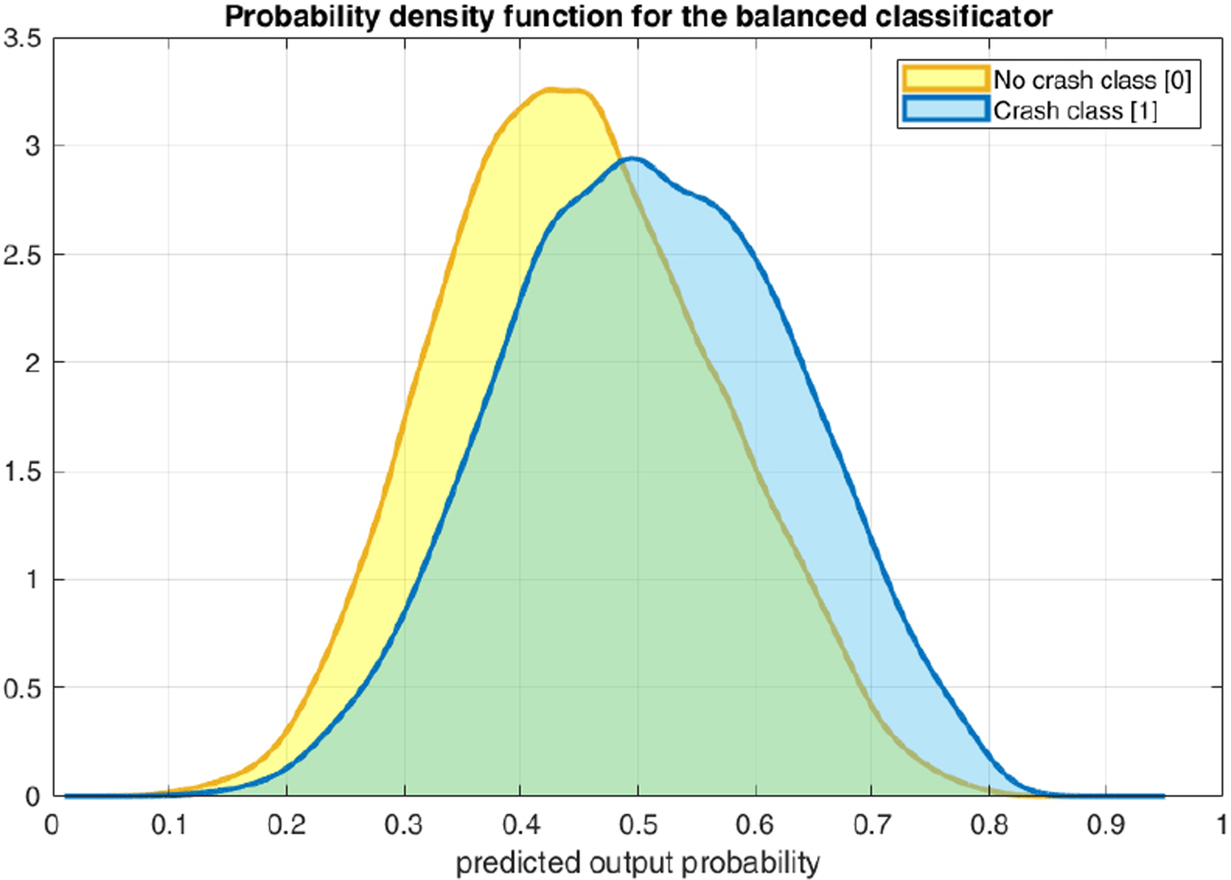
The cost-sensitive version of the Gradient Boosting algorithm is fed with a balanced version of the training data, therefore the out-of-sample predicted probabilities are centered at around 0.5 as depicted in Fig. 3.

The same model enhanced with the Platt scaling method, instead, provides output accident probabilities that are centered around 0.052, which is the real positive class prior probability. Figure 4 allows us to grasp very well, especially if compared with the previous one, the effect of this re-calibration of the probabilities in order to return to the real starting distribution 95%–5%.

The re-calibration through Platt scaling implies a threshold moving step. In a well-balanced binary classification task, when performing class assignment threshold is usually set at 0.5, which is the prior probability of observing the positive class. In the unbalanced context, after Platt scaling transformation of probabilities, this threshold is set at 0.052, which represents the prior probability for a vehicle to have an accident.

Figure 3.

Distribution of predictions before probability re-calibration.

Figure 4.

Distribution of predictions after probability re-calibration.

5. Crash prediction with static variates

5.1 Hardware requirements

The machine learning model runs on a Dell PowerEdge T640 server, featuring an Intel Xeon Silver 4214 Processor 2.20 GHz, which integrates 12 processing cores. The latter are independent central processing units within the CPU. The server has 16 GB RAM and a 2.4 TB HDD. Python was utilized to execute the algorithms and they have been developed to exploit the parallelization on the 12 cores.

The most critical part of defining the prediction model is the validation phase because it involves performing 10 iterations of the Gradient Boosting algorithm repeated 10 times (10-fold cross-validation). This process takes about 20 min and from here, the model’s hyperparameters and final features are fixed. Subsequently, when predicting the probability of an accident for a new vehicle, its probability of crash can be inferred in about 2 min.

5.2 Description of the process of building the prediction model

Before training the Cost-sensitive Gradient Boosting algorithm with static variates, a feature selection process is performed in order to select only the most meaningful features out of the 164 original ones and to guarantee the lowest possible computational load of the application.

The learning algorithm, as it is structured in levels, has the embedded possibility to output the list of input features with their ranking of importance in the data classification operation (while training), that is each feature’s information gain provided during the splitting of decision trees.

Feature importance can be used as the basis for the implementation of the Recursive Feature Elimination (RFE) procedure the following steps detail:

Start considering all 164 available features

Train Cost-sensitive Gradient Boosting with 10-fold cross-validation

Compute average feature importance and record 10-fold average AUC

Prune least important feature

Repeat process until only one feature remains

Select subset of features providing highest AUC

The algorithm employs the 10-fold cross-validation and the performance in terms of AUC and feature importance is obtained as an average of those on each of the 10 non overlapping folds.

Figure 5.

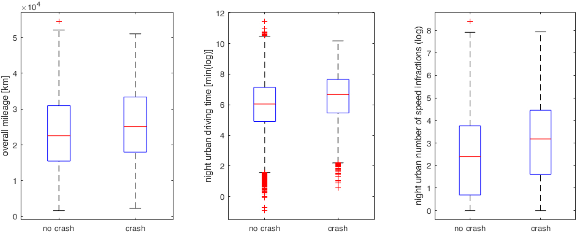
Boxplots of three of the most important static features with respect to the binary crash target class. Most interestingly, apart from the mileage traveled (left boxplot) which certainly increases the risk, it emerges that night driving time (center boxplot) and the number of speed offenses (right boxplot) both on urban roads are particularly capable of distinguishing the accident class from the non-accident class.

The RFE method brings to the selection of the optimal subset, containing 25 static features out of the 164 original ones. Figure 5 shows the univariate boxplot distribution of 3 of these 25 features, as an example. Vehicles which have been involved in accidents (no crash class) tend to drive more in terms of overall mileage, to drive more often during the night especially on urban roads and show a higher number of speed limit infractions than safe cars, in particular again during the night in the city. The Platt scaling version of the Cost-sensitive Gradient Boosting is trained based on the found subset of static 25 features, using a 10-fold cross-validation as well. The AUC is 0.640, while Balanced Accuracy is 0.600. Figures 3 and 4 show the distribution of the Platt scaling Gradient Boosting predictions (evaluated on the validation data) before and after the probability calibration process.

Interestingly, Fig. 6 highlights the significance of static features, which collectively contribute to 80% of the total importance (measured in terms of information gain) during machine learning training. Notably, features pertaining to urban mileage and driving during early morning or night emerge as the most crucial, underscoring the importance of segmenting data by road type and time of day. Comparatively, recent studies addressing Usage-Based Insurance (UBI) as a classification task have also predominantly focused on static features. For instance, [14] primarily utilize features based on distances, durations, and past accident records, achieving an AUC of 0.600 with a random forest model through 10-fold cross-validation. Similarly, [7] concentrate on distance, speed, and acceleration data, employing ensemble methods to achieve a peak AUC of 0.61 under similar validation conditions. [6], on the other hand, incorporate driving data, including accelerations, and accident responsibility information, reaching an AUC of 0.659 using logistic regression with a 10% hold-out validation approach. An outstanding accomplishment of this research lies in achieving state-of-the-art performance solely through cost-effective GPS driving data. Utilizing more advanced inertial sensors for measuring accelerations, for instance, would significantly escalate costs. Moreover, the study abstains from leveraging socio-demographic data about vehicles or drivers.

Figure 6.

Top static features accounting for 80% of total importance in order to predict accident risk. The uppermost metric, “Night Urban Mileage” is the most informative one, then passing to “Early Morning Urban Mileage”, and then to some overall quantities and moving on through “Early Morning Urban Number of Speed Infractions” and the subsequent ones.

Finally, it’s noteworthy that the aforementioned experimental investigation effectively identifies driving behaviors and conditions associated with heightened accident risks. These insights can inform the identification of risky factors and contribute to accident prevention efforts, encompassing variables such as total driving duration, time of day, and weather conditions, among others.

6. Crash prediction with additional dynamic variates

A set of 9 innovative features was identified as relevant information to be extracted from the built time series. However, computing these 9 quantities from each of the 164 time series for each vehicle would be too time and computing resources consuming and would result in an unmanageable input set of information.

The first pruning operation is then performed taking into account only the 25 time series corresponding to the optimal set of features found in the previous static feature selection. In this way, only the potentially most meaningful information is retained, avoiding an unnecessary workload and a too complex feature selection process. The extracted set of features accounts for 225 features (9 for each of the 25 time series) which could be further reduced to keep only really useful ones and improve performance. To accomplish this, a custom two-step feature selection is implemented for each of the 9 separate sets of 25 features:

Join together the considered set with the one of 25 static features, obtaining 50 mixed features.

Train the calibrated Cost-sensitive Gradient Boosting algorithm, evaluating AUC and Balanced Accuracy through 10-fold cross-validation.

If an improvement of performance with the mixed set with respect to the static one is present, then the 50 mixed features can be considered as a candidate set.

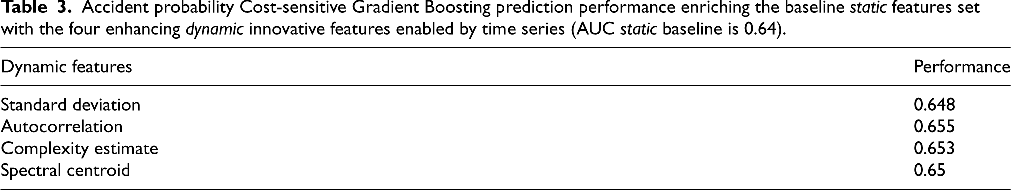
Among the 9 sets of features, only 4 of them bring to a significant improvement in performance as depicted in Table 3. The second step of feature selection consists of smartly combining all the identified best features, in order to build the final dataset and this process follows these stages:

All the identified candidate sets are joined together and with the static features set in a single dataset, resulting in a features space of 125 variables (25 standard deviations, 25 autocorrelations, 25 spectral centroids, 25 complexity estimates, 25 static features).

The resulting feature space is quite large and some variables could be meaningless or strongly correlated to each other. Therefore a RFE step is performed to find the best subset of features.

The returned subset of features represents the optimal final input dataset.

Table 3
Accident probability Cost-sensitive Gradient Boosting prediction performance enriching the baseline static features set with the four enhancing dynamic innovative features enabled by time series (AUC static baseline is 0.64).

Dynamic features Performance

Standard deviation 0.648

Autocorrelation 0.655

Complexity estimate 0.653

Spectral centroid 0.65

Dynamic features	Performance
Standard deviation	0.648
Autocorrelation	0.655
Complexity estimate	0.653
Spectral centroid	0.65

The RFE algorithm returns 68 features, including 15 standard deviations, 15 autocorrelations, 15 static features, 13 complexty estimates, 10 spectral centroids features, Fig. 7. This final dataset is used to train the usual custom Gradient Boosting algorithm, giving AUC $=$ 0.662 and a Balanced Accuracy of 0.620. The performance improvement when using features enabled by the inter-day time series representation of data is quite significant since the accident prediction task is inherently difficult. First, because the discovery of new relevant features is always hard and, second, because both the considerable natural imbalance and the strong overlapping between the two target classes makes even a one or two percentage point increase in the correctness of the output classifications extremely valuable. Table 4 shows a full comparison of the developed Machine Learning algorithm based on static metrics and on static variates enhanced with dynamic ones.

Figure 7.

Top dynamic features accounting for 80% of total importance for the prediction of accident risk. The uppermost metric, “Early Morning Mileage – standard deviation” is the most informative one, then passing to “Daily Vehicle Activity – autocorrelation”, and then to some specific quantities regarding mostly the night/early morning activity in various ways and again the urban environment.

Table 4

Comparative table on input features, classification method and performance of accident prediction based on static variates enhanced with dynamic ones.

Specifications	Static features	Mixed features
Period of observation	Two years	Two years
Feature engineering	Direct extraction from trips	Extraction from trips aggregated in time series
Type of features	Overall features (sum and means over 2 years)	Many time-series based features
Feature selection	Recursive feature elimination	Two-step feature selection
Final number of features	25	68
Training	Calibrated cost-sensitive GB	Calibrated cost-sensitive GB
Validation	10-fold cv	10-fold cv
Results (AUC)	0.64	0.662
Results (Balanced Accuracy)	0.60	0.62

A final consideration refers to Fig. 8 which depicts a pie chart graphically describing the percentage contribution to the target prediction added by each group of features. This allows to highlight the features importance and to capture at a glance that static metrics are crucial and account for a 19% of the information gain but, standard deviation and autocorrelation families of variates, just enabled by the time series representation of data, add about 30% informative content.

Figure 8.

Pie chart with the percentage of informative gain provided by each group of mixed features, static and time series enabled.

7. Concluding remarks

This paper has focused on developing an innovative UBI approach aimed at predicting the accident probability of private vehicles solely based on their driving behaviour, measured continuously in time and space by GPS equipped black boxes permanently installed on almost 100000 insured anonymized vehicles over a two years period.

A big dataset of millions of trips has been the starting point for the development of advanced Machine Learning algorithms, fulfilling the accident probability prediction task in the framework of complex Supervised Learning Binary classification algorithms, able to discriminate safe from risky vehicles, in a probability sense. The primary aim of our work was to employ intelligent Machine Learning techniques to extract all the predictive power from driving data and predict the crash probability even in the critical context of very unbalanced problems, like the one of car accident occurrence.

The Gradient Boosting classifier performance on the “static” features was evaluated on ROC AUC and Balanced Accuracy, guaranteeing a Balanced Accuracy of 0.6 and a AUC of 0.64. This last result represents a significant improvement over the existing literature: relevant studies report in fact similar or lower performance, but exploiting additional socio-demographic or acceleration/cornering information, which is instead supposed to be not available in our case. The first remarkable accomplishment of this work is therefore reaching the state-of-the-art using only primary and cheap driving behaviour telematics data.

As a secondary result, we showed that with a set of static/dynamic features, the same classifier performance improves: the AUC from 0.64 to 0.66 and the Balanced Accuracy from 0.60 to 0.62. This result represented a remarkable improvement, given the complexity of the learning task. We stress that our methodology is highly adaptable to various settings and geographical regions. The only requirement is to install a significant number of black boxes, potentially obtained from an insurance company, to accumulate a statistically significant dataset.

Footnotes

Acknowledgments

The authors thank UnipolTech and Unipol Group for the support and for providing a huge amount of private mobility data that enabled to train, validate and test the proposed Machine Learning Usage Based Insurance algorithms.

References

Tselentis

Yannis

Vlahogianni

E.I.

, Innovative motor insurance schemes: A review of current practices and emerging challenges, Accident Analysis and Prevention 98 (2017), 139–148.

Organization

W.H.

, Global status report on road safety, 2018.

Savaia

Formentin

Strada

Savaresi

, On the real range-need of electric cars: a telematic-box data-driven analysis, IFAC PapersOnLine 53(2) (2020), 14097–14102, 21st IFAC World Congress.

Zinnari

Strada

Tanelli

Formentin

Savaresi

, Electrification potential of fuel-based vehicles and optimal placing of charging infrastructure: A large-scale vehicle-telematics approach, IEEE Transactions on Transportation Electrification 8(1) (2022), 466–479.

Breschi

Ravazzi

Strada

Dabbene

Tanelli

, Fostering the mass adoption of electric vehicles: A network-based approach, IEEE Transactions on Control of Network Systems 9(4) (2022), 1666–1678.

Stankevich

N.P.N.

Korishchenko

Petrova

, Usage-based vehicle insurance: Driving style factors of accident probability and severity, Journal of Transportation Safety & Security 14(10) (2022), 1633–1654.

Huang

Meng

, Automobile insurance classification ratemaking based on telematics driving data, Decision Support Systems 127 (2019), 1–11.

Batista

Keogh

E.J.

Tataw

O.M.

de Souza

, CID: An efficient complexity-invariant distance for time series, Data Mining and Knowledge Discovery 14(10) (2013), 1633–1654.

Peeters

, A large set of audio features for sound description (similarity and classification) in the CUIDADO project, 2004.

10.

Schreiber

Schmitz

, Discrimination power of measures for nonlinearity in a time series, Phys. Rev. E 55 (1997), 5443–5447.

11.

Song

Zhang

, Fuzzy clustering-based adaptive regression for drifting data streams, IEEE Transactions on Fuzzy Systems 28(3) (2020), 544–557.

12.

Guo

H.Y.

Chen

, Understanding and modeling the human driver behavior based on MPC, IFAC Proceedings Volumes 46(21) (2013), 133–138, 7th IFAC Symposium on Advances in Automotive Control.

13.

Wahlstrom

Skog

Handel

, Smartphone-based vehicle telematics: A ten-year anniversary, IEEE Transactions on Intelligent Transportation Systems 18(10) (2017), 2802–2825.

14.

Baecke

Bocca

, The value of vehicle telematics data in insurance risk selection processes, Decision Support Systems 98 (2017), 69–79.

15.

Siami

Naderpour

, A mobile telematics pattern recognition framework for driving behavior extraction, IEEE Transactions on Intelligent Transportation Systems 22(3) (2021), 1459–1472.

16.

Leevy

J.L.

Khoshgoftaar

T.M.

Bauder

R.A.

Seliya

, A survey on addressing high-class imbalance in big data, Journal of Big Data 5(1) (2018).

17.

Mason

Baxter

Bartlett

P.L.

Frean

M.R.

, Boosting Algorithms as Gradient Descent, Neural Information Processing Systems, 1999.

18.

Cui

Jia

Lin

T.-Y.

Song

Belongie

, Class-Balanced Loss Based on Effective Number of Samples, in: 2019 IEEE/CVF Conference on Computer Vision and Pattern Recognition (CVPR), 2019, pp. 9260–9269.

19.

Niculescu-Mizil

Caruana

, Predicting good probabilities with supervised learning, 2005, 625–632.

20.

Platt

, Probabilistic outputs for support vector machines and comparisons to regularized likelihood methods, Adv. Large Margin Classif. 10 (2000).

Machine learning based car accident risk prediction for usage-based insurance

Abstract

Keywords

1. Introduction

2. Background and problem setting

3. Static and dynamic features engineering for measuring driving behavior

Table 1 Dataset overview before and after pre-processing. Geographic region Number of analysed vehicles Number of trips [ × 10 6 ] Italy Original 94268 426 Preprocessed 88120 395

4.1 The Machine Learning methodology

4.1.1 The class imbalance problem

4.1.2 Cost-sensitive Gradient Boosting learning framework

4.1.4 Probability calibration

5.1 Hardware requirements

5.2 Description of the process of building the prediction model

Footnotes

Acknowledgments

References

Table 1
Dataset overview before and after pre-processing.

Geographic region Number of analysed vehicles Number of trips $[\times 10^{6}]$

Italy Original 94268 426

Preprocessed 88120 395