Detection and classification of rice plant diseases

Abstract

Identification of diseases from the images of a plant is one of the interesting research areas in the agriculture field, for which machine learning concepts of computer field can be applied. This article presents a prototype system for detection and classification of rice diseases based on the images of infected rice plants. This prototype system is developed after detailed experimental analysis of various techniques used in image processing operations. We consider three rice plant diseases namely Bacterial leaf blight, Brown spot, and Leaf smut. We capture images of infected rice plants using a digital camera from a rice field. We empirically evaluate four techniques of background removal and three techniques of segmentation. To enable accurate extraction of features, we propose centroid feeding based K-means clustering for segmentation of disease portion from a leaf image. We enhance the output of K-means clustering by removing green pixels in the disease portion. We extract various features under three categories: color, shape, and texture. We use Support Vector Machine (SVM) for multi-class classification. We achieve 93.33% accuracy on training dataset and 73.33% accuracy on the test dataset. We also perform 5 and 10-fold cross-validations, for which we achieve 83.80% and 88.57% accuracy, respectively.

Keywords

Image segmentation machine learning classification disease classification disease detection disease segmentation rice disease

1. Introduction

Plant diseases are one of the causes in the reduction of quality and quantity of agriculture crops [22]. Reduction in both aspects can directly affect the overall production of the crop in a country [1]. The main problem is a lack of continuous monitoring of the plants. Sometimes newbie farmers are not aware of the diseases and its occurrence period. Generally, diseases can occur on any plant at any time. However, a continuous monitoring may prevent disease infection. The detection of a plant disease is one of the important research topics in the agriculture domain.

Figure 1.

Different types of rice diseases.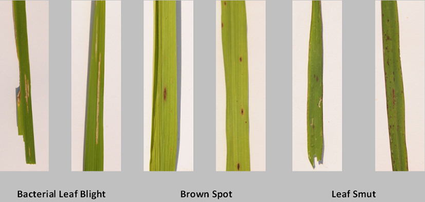

This article attempts to apply concepts of Machine Learning and Image Processing to solve the problem of automatic detection and classification of diseases of the rice plant, which is one of the important foods in India. On any plant, diseases are caused by bacteria, fungi, and virus. For rice plants, most common diseases are Bacterial leaf blight, Brown spot, Leaf smut, Leaf blast, and Sheath blight [18]. Image processing operations can be applied on external appearances of infected plants. However, the symptoms of diseases are different for different plants. Some diseases may have brown color or some may have a yellow color. Each disease has its own unique characteristics. Diseases differ in shape, size, and color of disease symptoms. Some of the diseases might have the same color, but different shapes; while some have different colors but same shapes. Sometimes farmers get confused and are unable to take proper decision for selection of pesticides.

Capturing the images of infected leaves and finding out the information about the disease is one way to get rid of loss of crop due to disease infection. As an automated solution of this problem, cameras can be deployed at certain distances in the farm to capture images periodically. These images can be sent to a central system for analysis of diseases; the system can detect the disease and give information about the disease and pesticide selection. At the core of such system would be to automatically recognize the disease that has occurred. We address this problem in this article. Objective of this work is to show how machine learning field can be useful for other discipline such as agriculture. An important part in applying machine learning field is to decide best features. Disease related features can only be extracted after segmenting disease and non-disease parts. An essential, reusable work of this article is to separate out leaf portion from disease part (majority of plants have leaves of green color), which we believe that is a crucial step in deciding the quality of features. Furthermore, the ideas presented in this work could also be applied to diseases that occur on other plants.

We briefly present our approach to solving the problem of automatic detection and classification of rice plant diseases. We collected the leaves from rice farm and prepared a dataset of images of rice plant leaves having a white background. Our system first removes the background from an image and then using K-means clustering it extracts the disease portions of the leaf image. After applying K-means clustering, some unnecessary green region is removed from disease portion using thresholding technique. We extract 88 chosen features from the diseased portion, and finally, we build Support Vector Machine (SVM) model to classify a disease.

This article is divided into seven sections. Section 2 presents a study on different types of rice plant diseases and discusses overall process of disease classification. Section 3 presents research that has already been done on rice plant disease detection and presents findings of the literature survey. Section 4 presents our proposed work. Section 5 presents detailed methodology we carried out in implementation and evaluation of our proposed work. Section 6 presents the experimental results. Finally, Section 7 summarizes the work in form of conclusion.

2. Background theory

This section provides domain understanding with a focus on (1) characteristics of different types of rice plant diseases and (2) the process of disease classification.

2.1 Different types of rice plant diseases

This section briefly describes the types of rice plant diseases considered in the research. The images of different diseases are shown in Fig. 1. Our work considers following three diseases: Bacterial leaf blight, Brown spot, and Leaf smut. Essential properties of these diseases are shown in Table 1.

Table 1
Different types of rice plant diseases and their essential properties

Sr. no.	Disease	Affected parts	Shape of symptoms	Lesion color
1	Bacterial leaf blight	Leaves	Elongated lesions, several inches long, on the leaf tip	Yellow to white due to the effect of bacteria
2	Brown spot	Leaves	Round to oval shapes	Reddish brown to dark brown
3	Leaf smut	Leaves	Small spots scattered throughout the leaf in non-uniform shape	Reddish brown

2.2 Overall process of classification

The process of detecting the plant disease based on the images is shown in Fig. 2. The process of getting images of infected leaves is referred as image acquisition.

Figure 2.

General approach of plant disease identification from the images.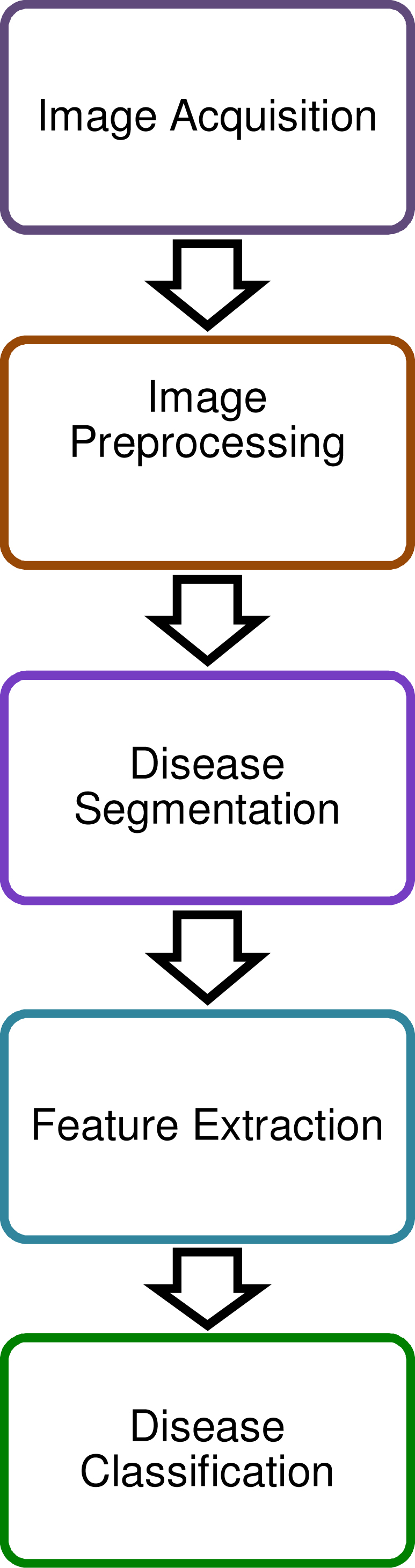

The process of plant disease detection is divided into two parts, image processing, and machine learning. The images are captured from the farm field. These images are further processed using image processing operations and at the end, machine learning model classifies the disease based on the image features. Various steps of image processing include image background removal, noise removal, image resizing, image segmentation, image feature extraction, while machine learning includes feature selection and classification. For different image dataset, techniques at each intermediate step might vary. For example, image resizing is not necessary every time, some image database contains images with low resolution. The evaluation of the system is carried out by the machine learning evaluation metrics such as accuracy, precision, recall, and confusion matrix.

3. Literature review

This section presents a concise survey of different image processing and machine learning operations applied in rice disease identification. A recent survey work in [19] has carried out detailed survey and analysis of various works in the same direction. For a related domain, a recent work in [16] has carried out detailed survey and analysis for cotton leaf diseases.

3.1 Survey and analysis of image processing operations applied for rice disease identification

In [23], three rice diseases: bacterial leaf blight, sheath blight, and rice blast were considered. Their work used 3 $\times$ 3 rectangular filter window to remove or weakened noises. After noise removal, the images were converted into two forms:

$\displaystyle y1=2g-r-b$ $\displaystyle y2=2r-g-b$

To segment disease spots from the rice leaf, their work used Otsu method. The shape and texture features were considered in their work [23] because the outside light highly influences color features. Their work used shape features such as area and perimeter. The texture features were obtained using gray level co-occurrence matrix. They used 4 shape features and 60 texture features.

In [2], disease segmentation was considered as a two class problem in which an image is treated as a matrix of M rows and N columns that can contain disease spot and natural part. Their work extracted color texture features using chromatography concepts of CIE XYZ color space and color features using CIE lab color space. The following shape features were considered in [2]: area, roundness, shape complexity, extending length and concavity, and equivalent rate of longer axis and shorter axis of the ellipse.

Pugoy and Mariano [17] used outlier detection method for detection of leaf scald disease of rice. The algorithm works in two phases. First, healthy and diseased images are prepared using HS histogram extraction and color extraction, respectively. Second, the disease is detected using test images. A research work in [3] used fermi energy based segmentation to extract the diseased parts from the images. Color features such as mean and standard deviation were extracted. The shape of the diseased part was extracted using DRLSE method [8]. The rough set theory was used for the reduction of computation time.

Suman and Dhruvakumar [21] used principal component analysis method to extract the shape features and 8-connected component analysis for the segmentation. Singh et al. [20] used wiener filter for removing blur and adaptive histogram for enhancing the contrast. Their work extracted only two features: entropy and standard deviation.

Figure 3.

Block diagram of the proposed work.

Phadikar et al. [13] used Otsu’s thresholding for the segmentation. Otsu’s thresholding requires gray scale image for which they used following equation to obtain the gray scale image.

$\textit{GreyScaleImage}=2(G-(0.75R-0.25B))$

Where R, G, B are the red, green, and blue planes, respectively. Images are further enhanced using a mean filter. Brown spot disease has different color intensity at the center and the boundary so that the radial distribution of the hue from the center to boundary was considered as a feature. Kahar et al. [6] used canny edge detection method. In their work, the images were first converted into gray scale, and then edges were detected. For image smoothing, they used erosion and dilation operations. For processing of disease part, they used color processing in LAB color space. Orillo et al. [12] carried out the conversion of RGB image to HSV in the preprocessing stage. They converted images into binary images using thresholding technique. They used blob extraction for removing noise. They used features such as a fraction of the diseased part, means of RGB values, and standard deviations of RGB components.

3.2 Survey and analysis of machine learning operations applied for rice disease identification

Yao et al. [23] used the SVM for classification of disease. In their work, total 72 images of each disease were divided into equal parts as training and testing samples. They created three classification models: (1) having 4 shape and 60 texture features, (2) having only 60 texture features, and (3) having only 4 shape features. They used radial basis kernel function in SVM. Anthonys and Wickramarachchi [2] used concepts of the membership function. The membership function is a function which defines the criteria for identification of disease. The membership function used in their research was as follows:

$\displaystyle\textit{MF}(\textit{RGB range, shape, length, width, diameter},$ $\displaystyle\quad\ldots)$

The classes were defined to evaluate the membership function. A test image was assigned to the class that has a higher membership value in evaluation. Charliepaul [3] used if-then classifier, in which if color and shape of a test image are same as that of a trained image, then that disease of trained image was classified for that test image.

Suman and Dhruvakumar [21] used SVM classifier. They used 60 samples for the classification purpose. The diseases considered in their work were bacterial Leaf blight, Brown spot, Narrow brown spot, and Rice blast. Amit Kumar Singh et al. [20] used SVM classifier which classified normal and diseased leaf into two different classes. They used K-means clustering for the segmentation of the image. Their classifier achieved an accuracy of 82%.

Phadikar et al. [13] used two approaches to classifying diseases: (1) the classification of normal and infected leaves and (2) classification between two or more diseased leaves. For classification, they used Bayes and SVM classifiers. They used 500 samples of each class in their work. Out of 500 samples, they used 450 samples for training and 50 samples for testing. In their work [13], 10 different combinations of training and test data resulted in an accuracy of 79.5%. Another classifier, SVM, achieved 68.1% accuracy with 10-fold cross validation. Kahar et al. [6] used back-propagation neural network, in which they used 3 output nodes for detecting three diseases: leaf blight, leaf blast, and sheath blight. Their work [6] used different samples taken in early, middle, and later stages of the diseases. They used a neural network as a classifier with sigmoid function as an activation function. Liu and Zhou [9] used total 400 images samples. They used back-propagation neural network for the classification. Orillo et al. [12] used 30 images for each disease. Their system used the back-propagation neural network for classification.

3.3 Findings from analysis

At each step of plant disease detection, various alternatives are available. Through a detailed study of different literature, we observed that there is no standard or benchmark image dataset available for the research. The authors in [2, 23, 13, 7, 11] specify that they created their own image dataset by capturing images from rice fields. After getting the images, image preprocessing is required for preparing images for further processing. Most of the authors [23, 21, 7] used a median filter to remove or weaken the noise from the images. The median filter is widely used for removing the noise, but in some cases when disease spots are too small, spots get blurred on the application of a median filter. There are also other filters used such as mean filter [13], laplacian filter [11]. Some authors, e.g. in [20], used histogram equalization technique to remove noise.

After preprocessing, extraction of disease portion from a leaf is done, which is referred as segmentation. Different techniques available for segmentation are Thresholding [2, 12], Otsu’s thresholding [23, 7, 13], Fermi energy based segmentation [3, 15], Entropy based bi-level thresholding [14], 8-conncted component labeling [21], and K-means clustering [20]. The next step is feature extraction from disease portion. The widely used features are (1) mean and standard deviation of R, G and B components of diseased portion [3, 20, 15], (2) area of diseased portion [2, 23], (3) texture features such as contrast, uniformity, and linear correlation [23].

The most widely used classifiers in literature are SVM [23, 13, 20, 10], neural network [9, 11, 6, 12], nearest neighbor [2], ensemble learning [10], quadratic discriminant analysis [10], IF-Then classifier [3], Bayes Classifier [13], and Rule Generation [15].

4. Proposed work

This section presents the proposed work for the rice disease identification. In our proposed system, we intend to detect three rice diseases namely Brown spot, Bacterial leaf blight, and Leaf smut. The block diagram of the proposed work is shown in Fig. 3. We discuss the processing steps of our proposed work in following subsections. We discuss higher-level steps of our proposed work in this section. Before arriving at a particular technique for performing a particular operation, e.g. disease segmentation, we have explored various alternative techniques. A detailed discussion of various techniques explored is presented in the next section.

4.1 Image acquisition

The images of rice plant leaves are captured from the farm field, which is needed when a dataset is not available. As rice crop requires a lot of water, majority farmers in India grow rice crop during rainy season, from July/August to October/November. In this season, there are high chances of bacteria, fungi, or virus affecting the crop. Therefore, we consider worst-case scenario for collected samples. We have collected leaves having varying degree of disease spread, which is essential for a dataset. We collected image samples from a village called Shertha near Gandhinagar, Gujarat, India. We captured images using NIKON D90 digital SLR camera with 12.3 megapixels in November 2015. The Dimensions of all images are 2848 $\times$ 4288 pixels. We had also taken some of the images from the related websites during preliminary study. We captured the images with a white background, in direct sunlight. We have prepared an image database of total 120 images, including 40 images of each disease. The format of all images is jpeg.

4.2 Image pre-processing

During processing in our system, we resize and crop the images into a dimension of 897 $\times$ 3081 pixels to reduce the memory requirement and computational power. Furthermore, an essential task is to remove the background from the image. We empirically explored four techniques to remove background from the leaf image: (1) apply mask generated based on original image, (2) apply mask generated based on Hue component values of the image in HSV color space, (3) apply mask generated based on Value component values of the image in HSV color space, and finally (4) apply mask generated based on Saturation component values of the image in HSV color space.

As shown in Fig. 3, the RGB image is converted into HSV color model. Next, because S component contains the whiteness, we choose saturation component of the HSV image for further processing. After that, we create a mask such that the mask removes and makes all the background pixel values to zeros, which represents black color, in RGB color space image. The background removed image contains only leaf portion, including disease spots.

4.3 Disease segmentation

We use K-means clustering for image segmentation. Three clusters are expected from a leaf image: (1) background, (2) diseased portion, and (3) green portion. We applied three image segmentation techniques to extract diseased portion from the leaf image: (1) LAB color space based K-means clustering, (2) Otsu’s segmentation technique, and (3) HSV color space based K-means clustering.

We use K-means clustering on the Hue component of the HSV image in our proposed work. For some images, normal K-means algorithm could not produce desired clusters, i.e., three segments. To produce accurate segments, we feed the centroid value of each desired cluster, which we find based on histogram analysis of Hue values of leaf portion. We use thresholding to remove the unnecessary green portion present in the diseased cluster, obtained as a result of K-means clustering.

Figure 4.

Flowchart for background removal.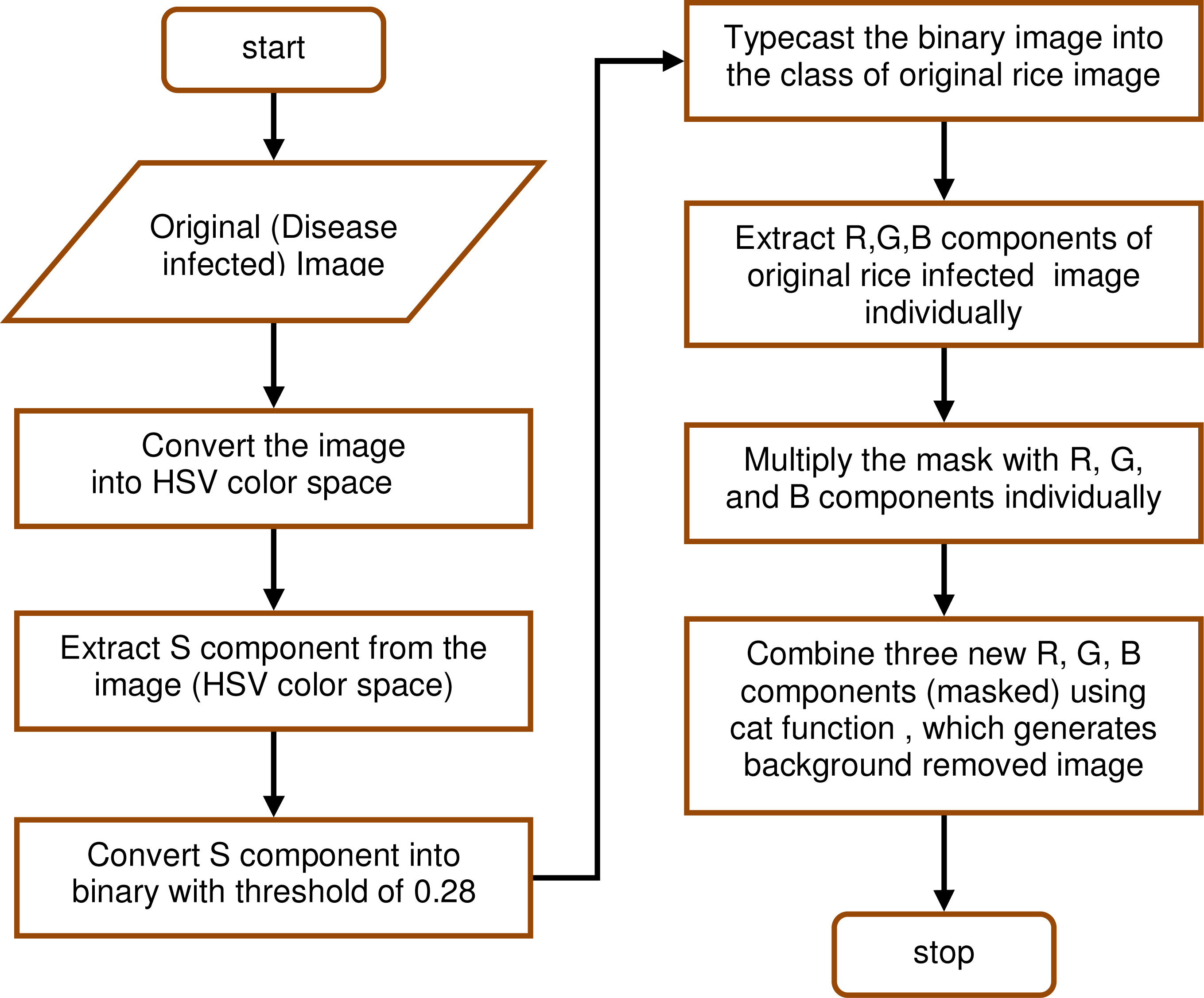

4.4 Feature extraction

Features have a crucial role in differentiating one disease from another. However, selection of features requires proper understanding and interpretation of feature values. We use various features under three categories: color, texture, and shape. In total, we have extracted 88 features from the disease portion of a leaf image.

Figure 5.

Results of background removal technique.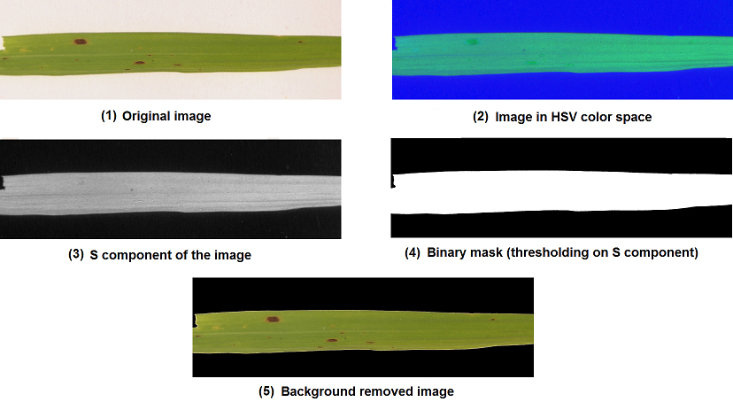

4.5 Classification

Preparation of dataset with known class labels is an essential step for classification of unknown data points. To assign class labels for collected leaf images, we had consulted the farmers and had asked them to provide names of diseases for sample leaves. Farmers had provided names in their native languages (Gujarati) and we identified and verified English names of those diseases by consulting with experts of an agriculture field. We use this prepared dataset for performing disease classification, for which we use SVM machine learning model. SVM is a supervised learning approach and does not suffer from the problem that occurs due to random weight assignments in Neural Network. It classifies the training data based on the classes given as training class labels. Linearly separable classes can be identified using a hyperplane while for the data points which are not linearly separable can be handled using appropriate kernel function. In our work, we have three classes (diseases). We use Gaussian kernel for multiclass classification.

5. Methodology: Detailed investigations and implementation

This section describes the detailed methodology of our proposed work. We also practically evaluate and discuss different alternatives we explored to arrive at the decision of choosing particular techniques, in our proposed work.

5.1 Background removal

The flowchart for removing the background is shown in Fig. 4 and results of intermediate steps for one sample image are shown in Fig. 5. We considered the background of images as white for which we captured the images by putting leaves on a white paper.

The disease infected leaf image is converted into HSV color space, refer the second image in Fig. 5. The saturation component of the HSV color space image is extracted, refer the third image in Fig. 5. We are not using hue component for background and shadow removal because hue contains pure color information without any brightness. We observed that shadow pixels do not contain any pure primary colors due to the absence of light in shadow regions. Whereas, the Value component contains lightness. It is only the saturation component that does not contain pure color, brightness, and lightness. After getting saturation component, the third image in Fig. 5, we convert it in a binary image with a threshold value of 0.28. The binary image has background pixels value zero, while leaf portion has pixel value one. We use this image, the fourth image in Fig. 5, as a mask to remove the background. We apply the binary mask on the original image, in RGB color space, to generate the background removed image, which is fifth image in Fig. 5.

5.2 Disease segmentation

To get an accurate diseased portion from a leaf image, we perform enhancement in the result of K-means by feeding centroid values of clusters. Furthermore, we also remove unnecessary green portions (leaf portion) from the disease cluster. Next, we discuss how we carried out segmentation of disease portion.

5.2.1 K-means clustering techniques for disease segmentation

We use K-means clustering for extracting the diseased portion from a leaf image. We generated three clusters having diseased portion, non-diseased portion, and background of the image. As LAB color space was used by many researchers for color image segmentation, we first tested rice disease infected images on LAB color space based K-means clustering [4]. The results showed that the algorithm cannot differentiate non-diseased and diseased portions accurately. We found that a large amount of green portions of leaf falls into the disease cluster. Thus, the LAB color space based K-means clustering could not produce effective output. Another problem in K-means clustering is the randomness of clusters, in which each time we run the algorithm, cluster centers get changed. As a result, the cluster that previously contained an infected portion of a leaf, now may not contain the infected portion in the next run. Therefore, we need to detect, out of three output clusters, which cluster represents the disease portion. We tried to detect the disease cluster by taking possible values of mean and standard deviation of each cluster’s R, G and B components, but we found that the values were overlapping among the clusters. Due to above problems in LAB based K-means clustering, we applied K-means clustering in HSV color space. We also empirically evaluated Otsu’s segmentation technique for disease segmentation.

Figure 6.

Flowchart of cluster centroid value estimation.

Figure 7.

Portion of the histogram of the H component of the background removed image.

Figure 8.

Histogram portion of the disease portion of the background removed image.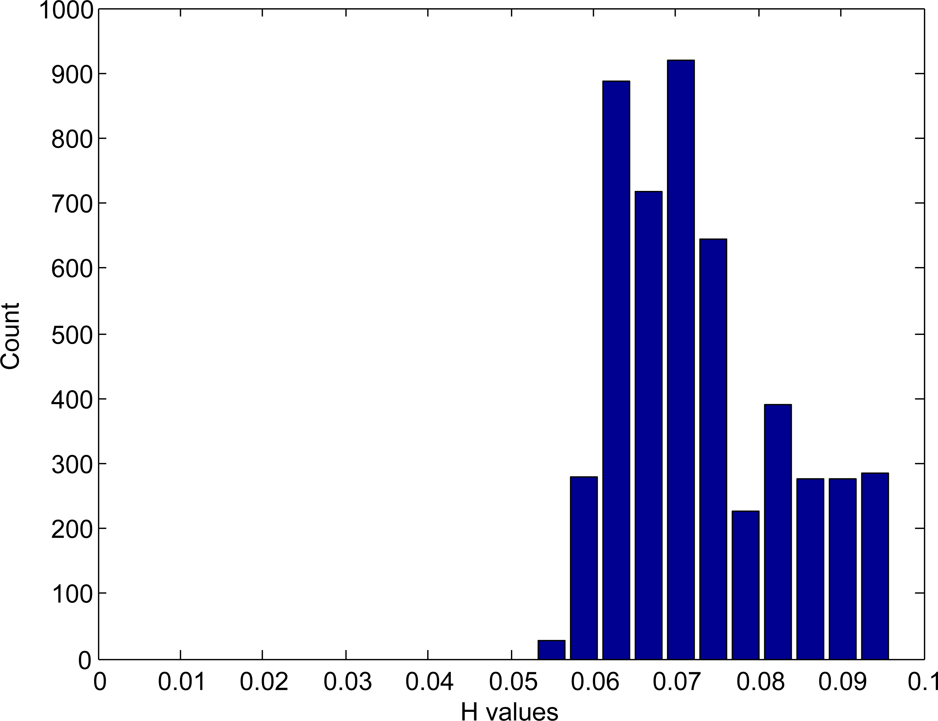

Figure 9.

Histogram portion of the non-disease portion of the background removed image.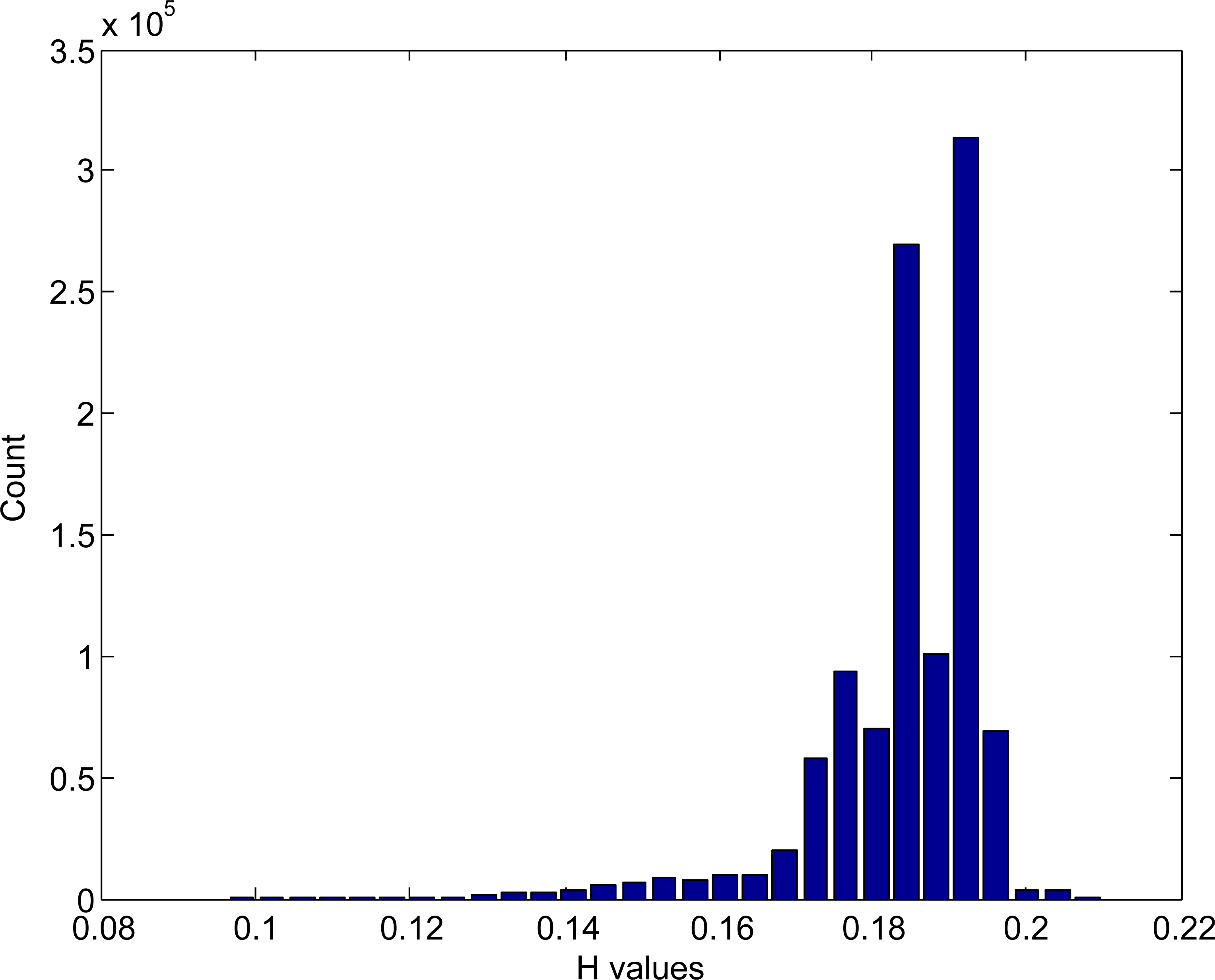

HSV color space contains hue, saturation, and value components. The hue component contains the pure color without any brightness and darkness information. We decided to apply K-means clustering on hue component, in HSV color space, of background removed image. To overcome the problem of the randomness of the cluster, we feed the initial centroid value of each cluster. Next, we discuss how we find initial centroid values.

Centroid value estimation: The flowchart of estimating centroid values of clusters is shown in Fig. 6. We first create the histogram of hue component of background removed image, in HSV color space. For one sample image, Fig. 7 shows the portion of the histogram of the H component of the background removed image. After that, we extracted the counts in each bin and values of hue component from the histogram. Based on the observation of disease infected image, and the histogram of a hue image, we found specific threshold value which can differentiate the diseased and non-diseased portions. Figure 8 shows the histogram portion of the disease portion for the sample image and Fig. 9 shows the histogram portion of the non-disease portion for the sample image. We store the hue values of bins of the diseased and the non-diseased portion of the image separately in two separate arrays. After getting the hue values of diseased and non-diseased portions, we select the maximum value from that range of values as a centroid value of each cluster, to be used in K-means clustering. We feed these two centroid values, for disease and non-disease portions, and value of black color, for background, in K-means clustering.

5.2.2 Applied K-means clustering for image segmentation

First, the image with background removal is converted into HSV color space. We applied K-means clustering on the hue component of this image. We have set the value of $K=3$ . Expected three clusters are (1) the diseased portion of a leaf, (2) the non-diseased portion, and (3) the background.

Matlab function for K-means takes a vector as input. However, we have the hue image, of two dimensions, which is a matrix. Therefore, we reshape the hue component, which is two-dimensional, using Matlab function reshape() into a vector. The kmeans() function returns the index value of each cluster. This function takes following parameters as input: vector of hue component, the value of K, and initial centroid value for each cluster. We create a labeled image, using reshape() function, having the same size as of original background-removed image by assigning cluster labels to each pixel. We now create three blank images with all pixel values as zeros, i.e., black colors, for storing three output clusters. Then, using labeled image we copy each pixel of an input image to appropriate cluster image. At the end of this step, we get three clustered images. The flowchart of our K-means Clustering is shown in Fig. 10. The results of K-means clustering on different rice disease images are shown in Fig. 11.

Figure 10.

Flowchart of K-means clustering for image segmentation.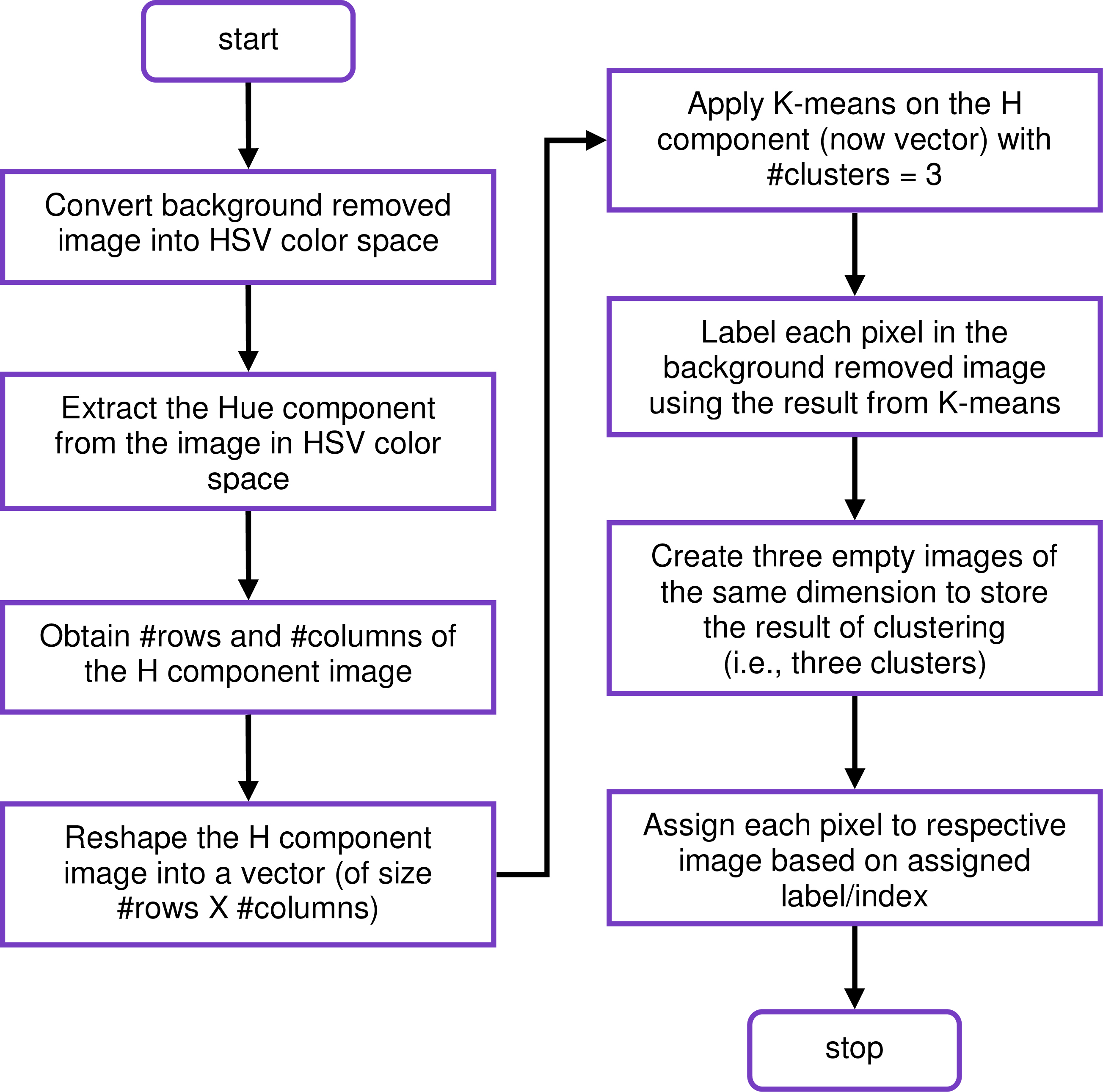

Figure 11.

Result of K-means clustering.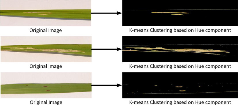

5.2.3 Removing green regions from disease cluster

We observed that at the end of K-means clustering, the disease cluster contained few green pixels in its surrounding, as shown in Fig. 12. The unnecessary green portion in the disease cluster can directly affect the accuracy of a classifier because these green pixels adversely contributes in calculations of features. We find that the green color falls between 17.2 degree to 45 degree in hue color wheel. These angle values map to 0.048 and 0.125, which we take as minimum and maximum values representing green colors. To remove unnecessary green pixels from the disease cluster, we created a binary mask based on these minimum and maximum values of hue component representing the range of green color. We used this mask in morphological operator (opening) to remove small unnecessary portions. However, due to noise present in the image, the image quality gets disturbed, some holes get generated within disease portion, which is shown Fig. 13. We fill such holes using region filling technique. The result of masking and removing green pixels from the disease portion is shown in Fig. 14.

Figure 12.

Green region in result of K-means clustering.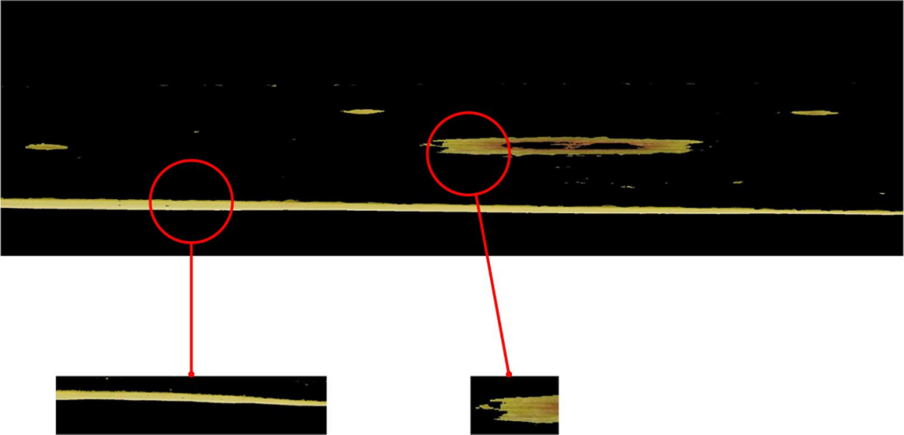

Figure 13.

Holes generated in result of K-means clustering.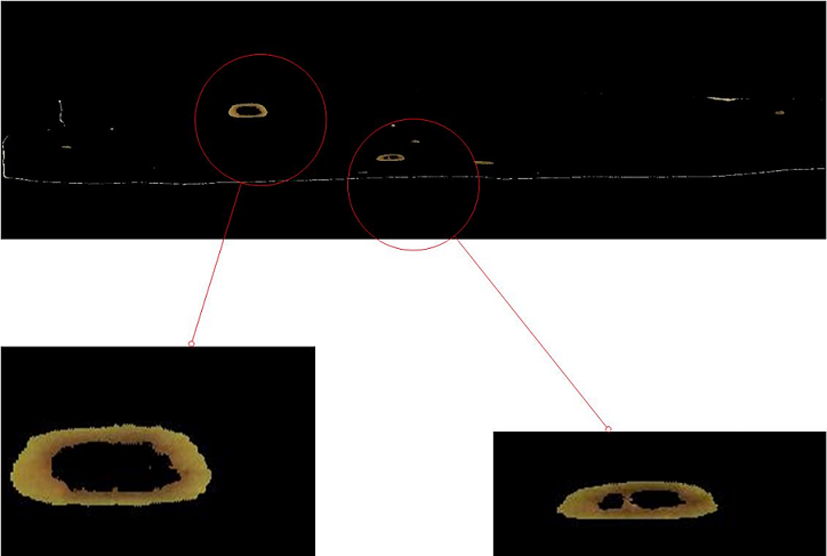

Figure 14.

Output of masking green region.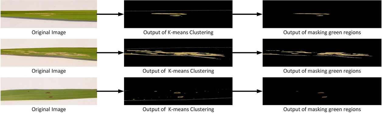

5.3 Feature extraction

We extract three categories of features: color, shape, and texture. We use following features in our work:

Color features: We extract following 14 color features of disease portion.

•
Mean values of nonzero pixels of R, G, and B components of the diseased portion in an image.
•
Mean values of nonzero pixels of H, S, and V components of diseased portion in HSV color space.
•
Mean values of nonzero pixels of L, A, and B components of diseased portion in LAB color space.
•
Standard Deviation of nonzero pixels of R, G, and B components of the disease portion of a leaf image.
•
Kurtosis.
•
Skewness.

Shape features: We extract following 4 shape features of disease portion.

•
Area of diseased portion.
•
The number of disease spots.
•
Minimum area of the obtained diseased spots.
•
Maximum area of the obtained diseased spots.

Texture features: We extract following 70 texture features of disease portion.

•
Contrast.
•
Correlation.
•
Energy.
•
Homogeneity.
•
Cluster Shade.
•
Cluster Prominence.
•
GLCM properties (contrast, correlation, energy, and homogeneity) in four directions (0, 45, 90, and 135 degrees), i.e., total 16 features $=$ 4 properties $\times$ 4 directions.
•
GLCM properties (contrast, correlation, energy, and homogeneity) of HSV components in four directions (0, 45, 90, and 135 degrees), i.e., total 48 features $=$ 4 properties $\times$ 4 directions $\times$ 3 planes (H, S, and V).

5.3.1 Extraction of color features

First, we extract the R, G, and B components of the image containing only diseased portion and store it into different variables. After that we extract only nonzero values and apply mean2() function of Matlab. The same process was repeated to find the mean values of H, S and V components of the image (in HSV color space) and for L, A, and B components of the image (in LAB color space). We apply std2() function of Matlab on nonzero values of R, G, and B color components.

5.3.2 Extraction of shape features

The total area of the disease portion of a leaf is calculated. It is calculated by converting the segmented image into binary with a threshold of 0.28 using Matlab’s inbuilt function im2bw(). This function gives output as a binary image containing 1’s and 0’s. After that area of binary image is calculated using bwarea() function.

The number of diseased spots is also one of the crucial features. It is calculated by using blob detection technique. Blobs are objects in a binary image. The Binary image of the diseased portion was used in finding the number of blobs in the image. The number of connected components is the number of diseased spots in the mask image. After that we found proportion area using following equation:

$\textit{Proportion∼{}area}=\frac{\textit{Area∼{}of∼{}each∼{}blob}}{\textit{% Total∼{}area∼{}of∼{}all∼{}blobs}}$

5.3.3 Extraction of texture features

We use Gray level co-occurrence matrix (GLCM) for extracting the texture features. GLCM contains the number of occurrences of each gray level in the image. Generally, GLCM scans the image in four different directions. We extract features by considering all directions. The Matlab function graycomatrix() was used to create the GLCM. The size of GLCM considered is 8 $\times$ 8. Using Matlab function called graycoprops(), we can find the values of all properties of GLCM which are contrast, correlation, energy, and homogeneity. We also calculate cluster shade and cluster prominence.

5.4 Classification

We prepare three classification models based on the number of features chosen. Model 1 consists of 88 features including 70 texture features, 14 color features, and 4 shape features. Model 2 consists of 72 features including 54 texture features, 14 color features, and 4 shape features. Model 3 consists of 40 features including 22 texture features, 14 color features, and 4 shape features. We manually provide labels to each disease, i.e., Bacterial leaf blight $=$ 1, Brown spot $=$ 2, and Leaf smut $=$ 3. We use Support Vector Machine (SVM) to generate three classification models for disease recognition. We use the libsvm library for classification. We use Radial Basis kernel function (Gaussian kernel). This kernel function is generally used for multiclass classification. We also observe the effect of different parameters of SVM such as cost and gamma on the accuracy of our classification models.

Figure 15.

Result of disease segmentation using HSV color space based K-means clustering.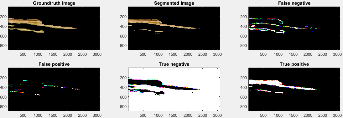

Figure 16.

Result of disease segmentation using LAB color space based K-means clustering.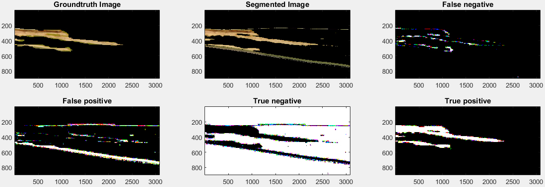

6. Experiments and results

This section presents different experiments we carried out in our work and the results we achieved.

6.1 Comparison of segmentation techniques

We use ground truth based approach to compare results of various segmentation techniques. Ground truth Image is an image in which segmentation can be done manually. In ground truth based approach, the result of segmentation is compared with the ground truth image [5]. We created the ground truth image by manually segmenting the disease portion from the leaf using Microsoft Paint tool.

We compare the performance of three segmentation techniques: (1) Otsu’s segmentation, (2) LAB color space based K-means clustering, and (3) HSV color space based K-means clustering. Different parameters to compare the segmentation result with reference to ground truth are as follows:

•
True Positive (TP): It indicates the intersection between the segmented portion and ground truth.
•
False Positive (FP): It indicates the segmented parts not overlapping the ground truth.
•
False Negative (FN): It indicates missed parts of the ground truth image in the segmented image.
•
True Negative (TN): It indicates the part of the image beyond the union of segmentation and ground truth.
•
Accuracy: An accuracy of segmentation technique can be calculated by the following equation:

$\textit{Accuracy}=\frac{\textit{TP}+\textit{TN}}{\textit{TP $+$ TN $+$ FN $+$ % FP}}$

Figure 15 shows the result of disease segmentation performed using HSV color space based K-means clustering. Figure 16 shows result of disease segmentation performed using LAB color space based K-means clustering. Figure 17 shows result of disease segmentation performed using Otsu’s segmentation technique.

Table 2
Results: Comparison of three segmentation techniques

Segmentation technique TP TN FN FP Accuracy (%)

1. HSV color space based K-means clustering 0.0588 0.9083 0.0265 0.0064 96.71

2. LAB color space base K-means clustering 0.0724 0.8554 0.0128 0.0593 92.79

3. Otsu’s segmentation 0.0586 0.8974 0.0267 0.0173 95.60

Figure 17.
Result of disease segmentation using Otsu’s segmentation technique.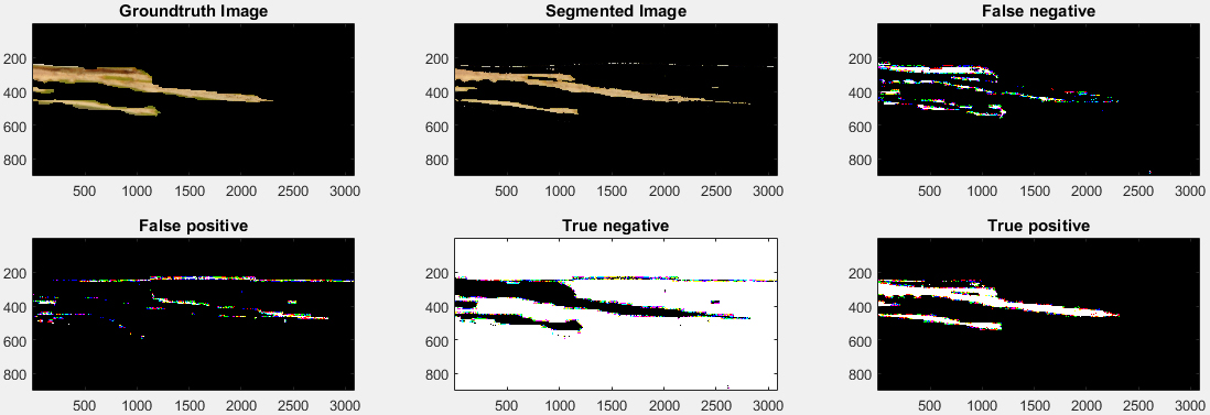

Table 2 shows a comparison of three segmentation techniques used for disease segmentation. It can be seen that HSV color space based K-means clustering provides highest accuracy among three methods. Therefore, we used this technique in our proposed work for disease segmentation.
6.2 Results: Effect of different parameters of SVM on classification accuracy

Segmentation technique	TP	TN	FN	FP	Accuracy (%)
1. HSV color space based K-means clustering	0.0588	0.9083	0.0265	0.0064	96.71
2. LAB color space base K-means clustering	0.0724	0.8554	0.0128	0.0593	92.79
3. Otsu’s segmentation	0.0586	0.8974	0.0267	0.0173	95.60

We create three classification models.

6.2.1 Model 1

Model 1 uses 88 features; these features are as follows: all 70 texture features, all 14 color features, and all 4 shape features (see Section 5.3 for details).

6.2.2 Model 2

Model 2 uses 72 features; these features are as follows: 54 texture features, all 14 color features, and all 4 shape features (see Section 5.3 for details). From all texture features, we exclude GLCM properties in four directions (i.e., 16 features).

6.2.3 Model 3

Model 3 uses 40 features; these features are as follows: 22 texture features, all 14 color features, and all 4 shape features (see Section 5.3 for details). From all texture features, we exclude GLCM properties of HSV components in four directions (i.e., 48 features).

We change cost and gamma parameters of SVM, and we perform 5-fold and 10-fold cross-validations. We train each model using 35 samples for each disease, and we perform testing using 5 samples of each disease. The effect of different SVM parameters on accuracies of three models is shown in Tables 3–5.

Table 3
Results: Effect of different SVM parameters on accuracy of the model having 88 features

						Training accuracy			Testing accuracy
Cost	Gamma	5-fold CV	10-fold CV	Training	Testing	BLB	BS	LS	BLB	BS	LS
(C)	(G)	accuracy	accuracy	accuracy	accuracy
2	0.5	85.71	88.57	98.09	66.66	97.14	97.14	100	80	80	40
2	0.125	85.71	86.66	90.47	73.33	94.28	91.42	85.71	100	80	40
128	0.125	87.61	87.61	100	66.67	100	100	100	100	80	20
2 ${}^{15}$	2 ${}^{-20}$	80.95	83.8	99.04	60	97.14	100	100	60	80	40
2 ${}^{15}$	0.5	85.71	88.57	98.09	66.67	97.14	97.14	100	80	80	40
2 ${}^{-20}$	0.125	85.71	86.66	90.47	73.33	94.2	91.42	85.71	100	80	40

Table 4

Results: Effect of different SVM parameters on accuracy of the model having 72 features

						Training accuracy			Testing accuracy
Cost	Gamma	5-fold CV	10-fold CV	Training	Testing	BLB	BS	LS	BLB	BS	LS
(C)	(G)	accuracy	accuracy	accuracy	accuracy
2	0.5	86.66	89.52	98.09	73.33	97.14	97.14	100	100	80	40
2	0.125	86.66	87.16	90.47	73.33	94.28	91.42	85.71	100	80	40
128	0.125	87.16	87.16	100	60	100	100	100	100	60	40
2 ${}^{15}$	2 ${}^{-20}$	80.95	82.85	99.04	60	97.14	100	100	60	80	40
2 ${}^{15}$	0.5	86.66	89.52	98.09	73.33	97.14	97.14	100	100	80	40
2 ${}^{-20}$	0.125	86.66	87.61	90.47	73.33	94.2	91.42	85.71	100	80	40

Table 5

Results: Effect of different SVM parameters on accuracy of the model having 40 features

						Training accuracy			Testing accuracy
Cost	Gamma	5-fold CV	10-fold CV	Training	Testing	BLB	BS	LS	BLB	BS	LS
(C)	(G)	accuracy	accuracy	accuracy	accuracy
2	0.5	83.8	88.57	93.33	73.33	94.28	91.42	94.28	100	80	40
2	0.125	81.9	81.9	89.52	73.33	94.28	91.42	82.85	100	80	40
128	0.125	88.57	87.61	99.04	66.66	97.14	100	100	100	60	40
2 ${}^{15}$	2 ${}^{-20}$	82.85	82.85	98.09	66.67	97.14	97.14	100	80	80	40
2 ${}^{15}$	0.5	83.8	88.57	93.33	73.33	94.28	91.42	94.28	100	80	40
2 ${}^{-20}$	0.125	81.9	81.9	89.52	73.33	94.28	91.42	82.85	100	80	40

Figure 18.

Class wise accuracy for Model 3.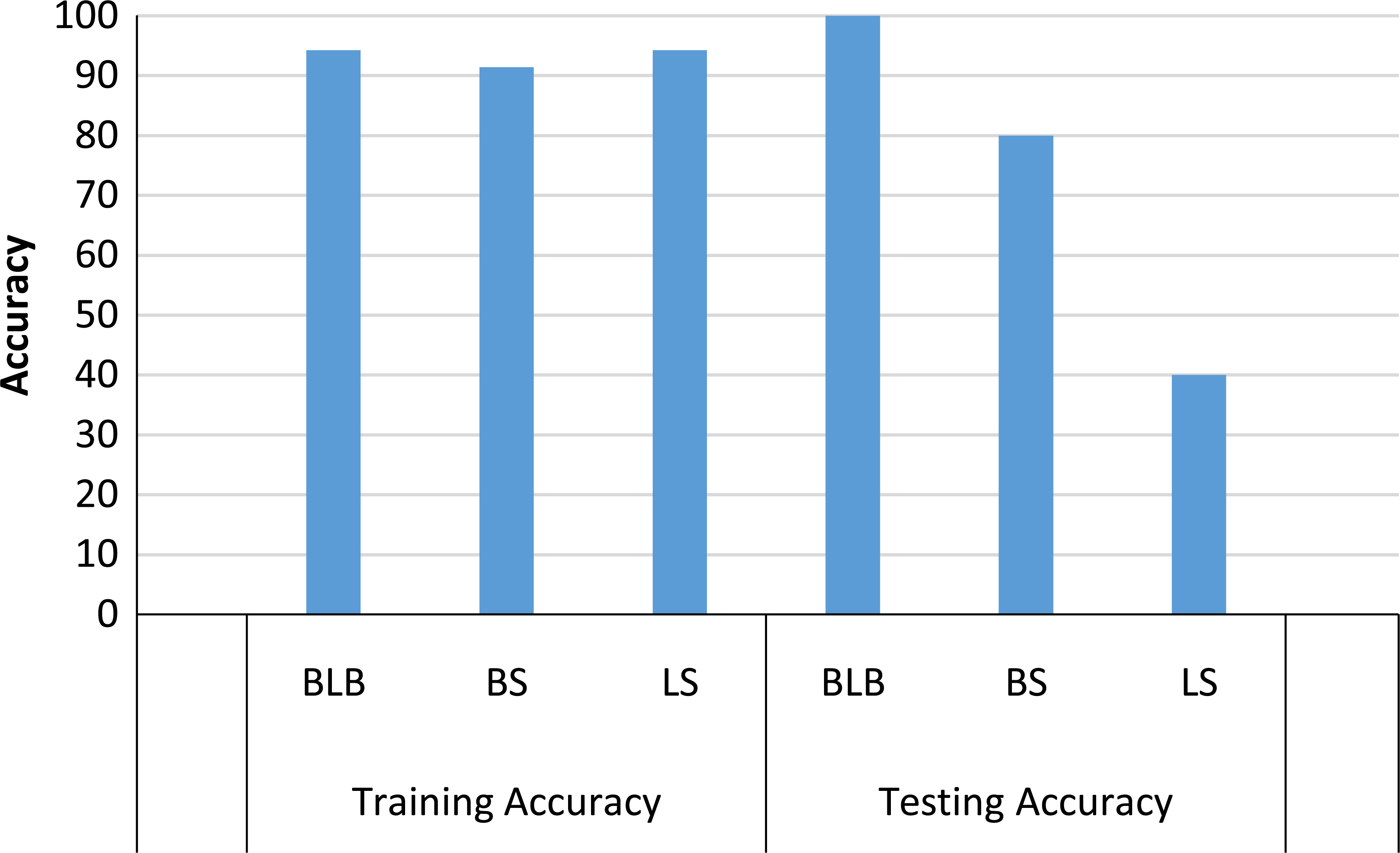

From the results presented in Table 3, we can see that different values of SVM parameters affect to training accuracy. We get lowest training accuracy of 90.47% and highest training accuracy of 100%. However, the quality of trained model is judged based on how it classifies unknown data. Highest testing accuracy was found to be 73.33%. We reduce the number of features and try to see its effect on training accuracy and testing accuracy. We find similar results for 72 features, presented in Table 4. We further try to reduce the number of features. Table 5 shows the effect of varying the SVM parameter on training and testing accuracies for Model 3, i.e., having only 40 features. We are able to achieve a highest testing accuracy of 73.33% even with only 40 features. Therefore, the results suggest that excluding the GLCM properties of HSV components in four directions does not degrade the testing accuracy. Thus, following texture features are sufficient to produce SVM classification model: Contrast, Correlation, Energy, Homogeneity, Cluster Shade, Cluster Prominence, and GLCM properties (contrast, correlation, energy, and homogeneity) in four directions (0, 45, 90, and 135 degrees).

We also need to evaluate how good a model can work for each class label. Figure 18 shows the class wise accuracy of each disease for Model 3. The figure shows both training and testing accuracies for the SVM parameters values $c=2^{15}$ and $\gamma=0.5$ . We observe that for Leaf smut disease class, the testing accuracy is only 40%, which is very low. The possible reason for this low testing accuracy might be due to confusion between Brown spot and Leaf smut diseases. In Fig. 1, we can see that both Brown spot and Leaf smut have spots or regions of brown color.

6.3 User interface of the system

The user interface of the system contains two parts: Training and Testing GUI. Training GUI, shown in Fig. 19, takes images of different diseases as input and provides the trained SVM model as output, which can be written to a file for use in testing GUI. Using this GUI, the user can specify class label of images while inputing the images. This GUI has three buttons using which we can initiate following operations: (1) Remove Background, (2) K-means Clustering, and (3) Mask Green Regions. The training GUI also allows selection of features to be included in the trained model.

Testing GUI, shown in Fig. 20, takes following as input: a single image of rice leaf, infected with an unknown disease and the model generated via the Training GUI. This easy-to-use GUI helps in understanding all intermediate steps performed from image input to disease classification.

Figure 19.

Main screen of training GUI.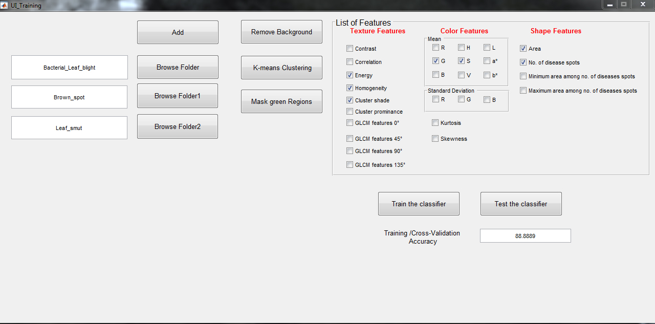

Figure 20.

Main screen of testing GUI.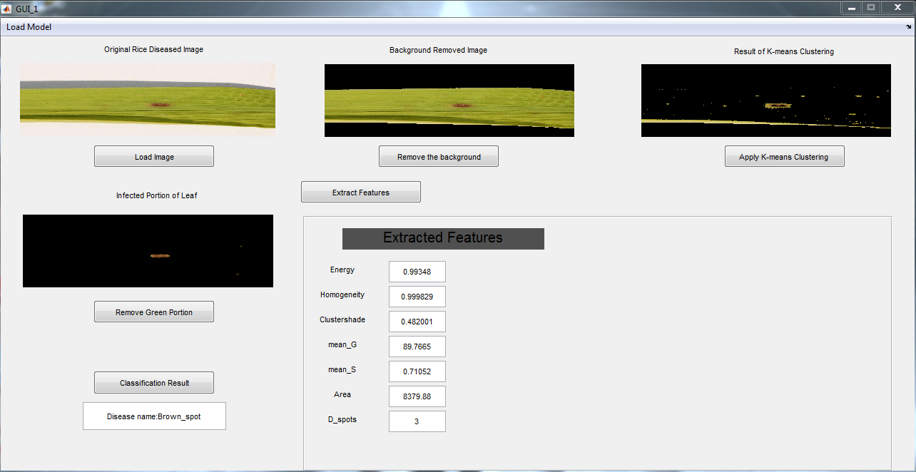

In summary, this work has experimentally evaluated four techniques of background removal and suggested to use S component based background removing technique for the images in our dataset. For segmenting disease portion from leaf portion, this work evaluated three image segmentation techniques: (1) LAB color space based K-means clustering, (2) Otsu’s segmentation technique, and (3) HSV color space based K-means clustering. This work proposed the use of HSV color space based K-means clustering with feeding centroid values to achieve accurate segmentation of disease. This work built and experimentally evaluated three models having a varying number of features. The results suggested using Model 3 having only 40 features rather than the initial model, Model 1, having 88 features. In future, we would like to use or make larger image dataset for rice plant diseases. Furthermore, we would like to improve accuracy on test images, more specifically, for Leaf smut, for which accuracy on test images was found to be low as 40%. We would also like to observe the effect of making model still simple by reducing features under the color category. Furthermore, we would also like to differentiate Leaf smut disease from Brown spot, for which adding shape based features might help.

7. Conclusion

Rice plant diseases can make a big amount of loss in the agriculture domain. This article presented a system to detect and classify three rice plant diseases, including Bacterial leaf blight, Brown spot, and Leaf smut. We prepared our own dataset of leaf images by gathering leaves from a rice field in a village called Shertha near Gandhinagar, Gujarat, India. We experimentally evaluated all possible techniques in image processing part. We experimentally evaluated various background removal techniques. Finally, we showed that the background of an image gets accurately removed by applying the mask created by thresholding on the saturation component of the original image in HSV color space. We experimentally evaluated various segmentation techniques to segment disease portion. We used K-means clustering with feeding centroid values for disease segmentation. We removed unnecessary green portions from the disease cluster by applying thresholding on the hue component of disease portion. We found that our selected image processing operations prepared images suitable for extraction of features. We extracted total 88 features and considered three different models having a different number of features.

We used SVM to classify the disease and we achieved 93.33% training accuracy and 73.33% testing accuracy. We also performed k-fold cross validation for $k=$ 5 and $k=$ 10. We also developed easy-to-use GUI for understanding all intermediate steps performed from image input to disease classification. Our future work would concentrate on improving the background removal technique, which can work on a real field background. Furthermore, in machine learning part, we intend to apply other classifiers such as rule-based classifier and K-nearest neighbor for classification of rice plant diseases. In future, we would like to improve accuracy on test images. More specifically, accuracy on test images for Leaf Smut was found to be low comparatively. Therefore, we plan to explore other features based on which Leaf smut can be distinguished from Brown spot. In India, in last few years even an ordinary person has started using a smart phone, having Internet connectivity. If this work can be hosted as web-services, its access could become very useful to farmers. In future, it might be possible for farmers of India to avail such facility via realization of Digital India mission of the country. In making this work accessible through a smart phone, we are working on developing an Android Application using OpenCV.

References

Al Bashish

Braik

Bani-Ahmad

. A framework for detection and classification of plant leaf and stem diseases. In Signal and Image Processing (ICSIP), 2010 International Conference on IEEE 2010 Dec 15; 113-118.

Anthonys

Wickramarachchi

. An image recognition system for crop disease identification of paddy fields in Sri Lanka. In Industrial and Information Systems (ICIIS), 2009 International Conference on IEEE 2009 Dec 28; 403-407.

Charliepaul

. Classification of rice plant leaf using feature matching. International Journal on Engineering Technology and Sciences 2014; 1(2): 290-295.

Color-Based Segmentation Using K-Means Clustering – MATLAB & Simulink Example – MathWorks India. Last accessed on 13 May 2016. url: http://in.mathworks.com/help/images/examples/color-based-segmentationusing-k-means-clustering.html.

Jiang

Marti

Irniger

Bunke

. Distance measures for image segmentation evaluation. EURASIP Journal on Applied Signal Processing 2006 Jan 1; 2006: 209.

Kahar

Mutalib

Rahman

. Early detection and classification of paddy diseases with neural networks and fuzzy logic. In 17th International Conference on Mathematical and Computational Methods in Science and Engineering (MACMESE’15) 2015; 248-257.

Kurniawati

Abdullah

. Investigation on image processing techniques for diagnosing paddy diseases. In Soft Computing and Pattern Recognition, 2009, SOCPAR’09, International Conference of IEEE 2009 Dec 4; 272-277.

Gui

Fox

. Distance regularized level set evolution and its application to image segmentation. IEEE Transactions on Image Processing 2010 Dec; 19(12): 3243-3254.

Liu

Zhou

. Extraction of the rice leaf disease image based on BP neural network. In Computational Intelligence and Software Engineering, 2009 CiSE 2009, International Conference on IEEE 2009 Dec 11; 1-3.

10.

Maharjan

Takahashi

Zhang

. Classification methods based on pattern discrimination models for web-based diagnosis of rice diseases. Journal of Agricultural Science and Technology 2011; 1(1): 48-56.

11.

Majid

Herdiyeni

Rauf

. I-PEDIA: Mobile application for paddy disease identification using fuzzy entropy and probabilistic neural network. In Advanced Computer Science and Information Systems (ICACSIS), 2013 International Conference on IEEE 2013 Sep 28; 403-406.

12.

Orillo

Cruz

Agapito

Satimbre

Valenzuela

. Identification of diseases in rice plant (oryza sativa) using back propagation Artificial Neural Network. In Humanoid, Nanotechnology, Information Technology, Communication and Control, Environment and Management (HNICEM), 2014 International Conference on IEEE 2014 Nov 12; 1-6.

13.

Phadikar

Sil

Das

. Classification of rice leaf diseases based on morphological changes. International Journal of Information and Electronics Engineering 2012; 2(3): 460.

14.

Phadikar

Sil

. Rice disease identification using pattern recognition techniques. In Computer and Information Technology, 2008, ICCIT 2008, 11th International Conference on IEEE 2008 Dec 24; 420-423.

15.

Phadikar

Sil

Das

. Rice diseases classification using feature selection and rule generation techniques. Computers and Electronics in Agriculture 2013; 90: 76-85.

16.

Prajapati

Dabhi

Prajapati

. A survey on detection and classification of cotton leaf diseases. In Electrical, Electronics, and Optimization Techniques (ICEEOT), International Conference on IEEE 2016 Mar 3; 2499-2506.

17.

Pugoy

Mariano

. Automated rice leaf disease detection using color image analysis. In 3rd International Conference on Digital Image Processing, International Society for Optics and Photonics 2011 Apr 15; 80090F-80090F.

18.

Rice Production (Peace Corps): Chapter 14 – Diseases of rice. Last accessed on 23 November 2015. url: http://www.nzdl.org.

19.

Shah

Prajapati

Dabhi

. A survey on detection and classification of rice plant diseases. In Current Trends in Advanced Computing (ICCTAC), IEEE International Conference on IEEE 2016 Mar 10; 1-8.

20.

Singh

Rubiya

Raja

. Classification of rice disease using digital image processing and svm classifier. International Journal of Electrical and Electronics Engineers 2015; 7(1): 294-299.

21.

Suman

Dhruvakumar

. Classification of paddy leaf diseases using shape and color features. International Journal of Electrical and Electronics Engineers 2015; 7(1): 239-250.

22.

Weizheng

Yachun

Zhanliang

Hongda

. Grading method of leaf spot disease based on image processing. In Computer Science and Software Engineering, 2008 International Conference on IEEE 2008 Dec 12; 6: 491-494.

23.

Yao

Guan

Zhou

Tang

Yang

. Application of support vector machine for detecting rice diseases using shape and color texture features. In Engineering Computation, 2009, ICEC’09. International Conference on IEEE 2009 May 2; 79-83.

Detection and classification of rice plant diseases

Abstract

Keywords

1. Introduction

2.1 Different types of rice plant diseases

Table 1 Different types of rice plant diseases and their essential properties

3.1 Survey and analysis of image processing operations applied for rice disease identification

3.3 Findings from analysis

4. Proposed work

4.1 Image acquisition

4.2 Image pre-processing

4.3 Disease segmentation

5. Methodology: Detailed investigations and implementation

5.1 Background removal

5.2 Disease segmentation

5.2.1 K-means clustering techniques for disease segmentation

5.3.2 Extraction of shape features

5.3.3 Extraction of texture features

5.4 Classification

6.1 Comparison of segmentation techniques

6.2.1 Model 1

6.2.2 Model 2

6.2.3 Model 3

Table 3 Results: Effect of different SVM parameters on accuracy of the model having 88 features

References

Table 1
Different types of rice plant diseases and their essential properties

Table 3
Results: Effect of different SVM parameters on accuracy of the model having 88 features