An algorithm for Elliott Waves pattern detection

Abstract

The examination of the Elliott Wave theory is the main motivation of this contribution. All of the fundamental features of an proper Elliott Wave pattern (EW pattern) are reviewed and explained. Based on this knowledge, an algorithm for detection of these patterns is designed, developed and tested. Under several different algorithm settings, several EW pattern sets are obtained. They differ in amount of found EW patterns, quality and size.

The following application of the developed detection algorithm was based on recognition of an incomplete EW patterns with aim of the prediction of the following progress of the time set. The Random Decision Forest and the Support Vector Machine are the machine learning algorithms employed for this task. The accuracy of trend prediction above 70% proves the relevancy of EW patterns on stock market data as well as the validity of the algorithm as a tool for detection of such patterns.

Keywords

Time series forecasting Elliott waves stock markets support vector machine random forest

1. Introduction

The behavior of stock market price is a reflection of complex interactions of multiple underlined processes like political statements, macroeconomic situation, news, investors psychology, previous behavior of the price itself, etc. These interactions bring huge amount of noise, uncertainty and non-rational moves into the price progress which makes it difficult to forecast.

The Efficient Market Hypothesis (EMH) is one of the most known ideology connected with predictability of the stock market price behavior [1]. EMH simply denies its possibility. Market price, in the view of this hypothesis, is an absolutely rational reflection of all inner and outer influences as well as all available information without any misunderstandings or misinterpretations. Such a statement describes the market as unpredictable. Because EMS contains several empirical drawbacks [2] and also some very first attempts proved that well designed predictive model is able to proceed much better forecasting [3, 4, 5] than random walk [6], the market is mostly not considered as fully efficient and unpredictable.

There are many high quality studies aiming into this topic with application of ML [7, 8, 9]. The movement prediction with widely known Support Vector Machine obtained interesting results in study of Huang et al. [10]. The application of neuro-fuzzy system in the study of Atsalakis et al. [11] brought results of comparable quality. The next proposal combining the Genetic Algorithm and Support Vector Machine was tested also with success in study of Choudhry [12]. The application of robust random number generator showed its purpose in several studies [13, 14] and also experiment proposed in this contribution relies on application of Mersenne Twister approach [15]. All of these models faced with different conditions (time series length, chosen markets, length of forecast, etc.) but most of them comes with similar results which confirms the difficulty of forecasting of the stock market direction.

Figure 1.

Up-trending (right) and down-trending (left) waves recognized on EURUSD market with 15 minute time scale and 10% tolerance.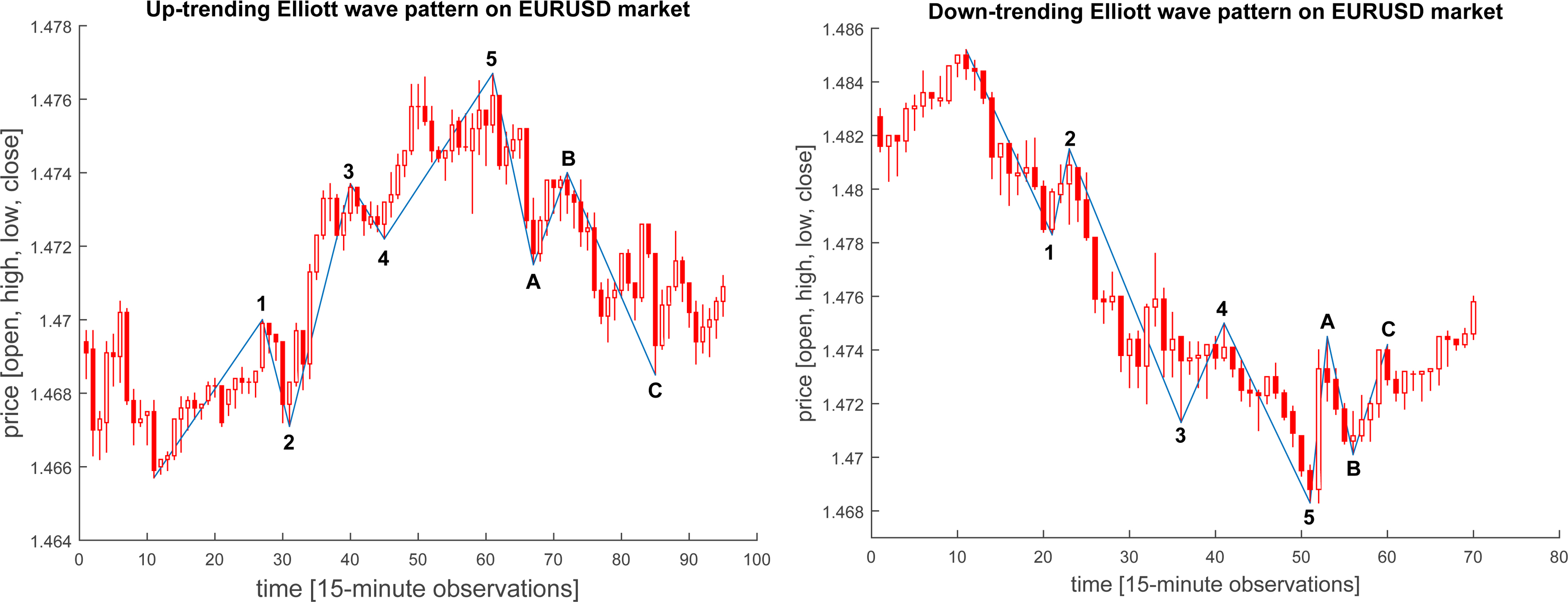

The high quality reviewing study brought by Soni [16]

concludes the strong predictive ability of Artificial Neural Network as a computational model in this task. In [17], Atsalakis and Valavanis conclude that soft-computing models such as ANN and Neuro-fuzzy models are able to outperform the conventional models in most cases, as well as the study by Yoo et al. [18]. The wider review brought by Enke and Thawornwong [19] describes also the influence of statistical relations between different economic variables valuable for the forecasting.

Based on these studies, the market can be definitely considered as a predictable as well as by the proposal of Elliott, which brought the theory of Elliott Wave patterns in 1946 [20]. He described how every stock market repeats itself in some predictable patterns, so called waves. The application of Elliott waves, recognized by Artificial Neural network proposed by Volna et al. [21] includes several tests for its predictability performance as well.

This paper describes our algorithm for EW pattern detection, that is based on hard-coded rules. The information background of the EW’s theory, the work-flow of the algorithm as well as the platform ans programming language are covered in the first part of the paper. The following parts describe the experimental application of the algorithm on real stock market data. The EW patterns are extracted on several different adjustments and they are examined on the fitting to the defined rules. In the further step, the selected patterns serve as input values for the trend prediction models based on machine learning algorithms. The final discussion covers advantages and disadvantages of the model as well as the future research.

Figure 2.

UML diagram of EW pattern detection algorithm. Described process examines all IFs in a given time set window and returns the matrix of found EW patterns with their fitness values.

1.1 Elliott wave theory

This theory defines the basic pattern of five motive and three corrective waves, which appears in both trend directions, bearish and bullish. These patterns posse the feature of “self-similarity”, which means that the same pattern can be observed in sub-parts of the entire EW. This feature is a sign of fractal behavior of the EW’s pattern. The form of the waves is very consistent and it follows Fibonacci’s ratios, which is one of the major guide line of their detection.

This proposal of Elliott Waves (EW) is still an active area of study and it was reviewed and extended by many authors [22, 23]. The EW’s patterns were many times the motivation of application of algorithmic pattern recognition based on fuzzy logic or artificial neural networks [24, 21]. The proper identification of the actual wave can be considered as the ideal tool for prediction of the future price move and final profit target placement [25, 26].

For proper indentification of the EW pattern, it has to be considered three major rules [22, 23]

1.
The second wave never ends below the starting point of the first wave.
2.
The third wave is never the shortest wave.
3.
The wave four never ends in the price are of the fist wave.

and rules based on Fibonacci ratio’s.

1.
The length of wave 2 is from 50% to 62% of the wave 1.
2.
The wave 3 can be 1.62, 2.62 or 4.25 longer than wave 1.
3.
The wave 4 is retracing from 24% to 38% of the wave 3.
4.
The wave 5 is the multiplication of 1, 1.62 or 2.62 and wave 1.
5.
The wave A is almost equally length as the wave 5.
6.
The wave B is retracing from 50% to 76.8% of the wave A.
7.
The wave C can be length of 0.62, 1 or 1.62 times wave A.

2. Algorithm design

The EW detection algorithm described in this study is based on hard-coded rules with adjustable set of coefficients representing fuzzy tolerances in pattern detection process. The UML diagram of the algorithm is depicted in Fig. 2.

Figure 3.

Up initiating fractals examples, source “Trading Chaos” [27].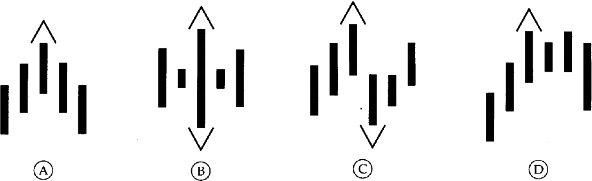

2.1 Initialization

There are several very important variables that serves as the inputs of the algorithm. The first is the vector $X$ that is the non-stationary, trend-full time set. The time series should not be pre-processed, de-noised or filtered, because the algorithm attempts to find EV’s of all of the possible sizes. The $X$ is divided into smaller windows of length $w$ . For each of the window, there is initiated parallel process which can run independently. The second input variable is the tolerance vector $t$ . This vector of double values represents tolerances for the wave-selection process.

At the start of the process there are initialized two vectors $L_{\min}$ and $L_{\max}$ which hold the indexes of the local minimums and maximums of the input time set. These kind of extremes are titled as “Initiating Fractals” (IF) and firstly were introduced in Dr. Bill Williams’ book “Trading Chaos” [27]. The basic definition of IFs deals with defined width (number of ticks accounted into structure) and if the high in the middle is the highest high of the structure, than it is ‘up’ fractal, otherwise ‘down’ fractal (see in Fig. 3). The process than iterates the IFs multiple times with attempt to find the best combinations which could probably represent the EWs.

2.2 Pattern selection

Up-trending EW starts in the down IF, therefore the process iterates all of the indexes from $L_{\min}$ and applies them as IFs of the EW. On the other hand the down-trending EW starts in the up IF, so the process iterates $L_{\max}$ as its IFs.

The process comes through both local extremes to complete the entire wave pattern and in every time the process looks for the best matching opposite extreme which can fit to the defined rules with adjusted level of tolerance. The application of tolerances can be generically described by following equations.

$\displaystyle I_{up}=W_{j}\times(F_{j+1}\times(1+t_{j+1}))$ (1) $\displaystyle I_{down}=W_{j}\times(F_{j+1}\times(1-t_{j+1}))$ (2)

where $I_{up}$ and $I_{down}$ is a couple of upper and lower boundaries for the following wave, $W$ is the price-level of the $j$ -th wave, $F$ is the applied Fibonacci ratio (according to the rules) and $t$ is the value of defined tolerance for the upcoming wave.

Every time the fractal structure can be connected to more possible fractal structures and all of this combinations are stored in stack and used in next step as valid sub-waves. When the fractal can not connect to its next follower, the entire sub-wave in deleted from the stack. During every step, some of the sub-waves which can grow multiple ways are multiplied and others, which are not able to grow anywhere are removed. When the last fractal is added into the sub-pattern, the complete EW is found (under the certain level of tolerance) and it is saved in the output matrix M. In the end of the process, the matrix M can contain similar and overlapping patterns which has to be handled before the process terminates.

Figure 4.

Up-trending (right) and down-trending (left) waves recognized on EURUSD market with 15 minute time scale and 10% tolerance.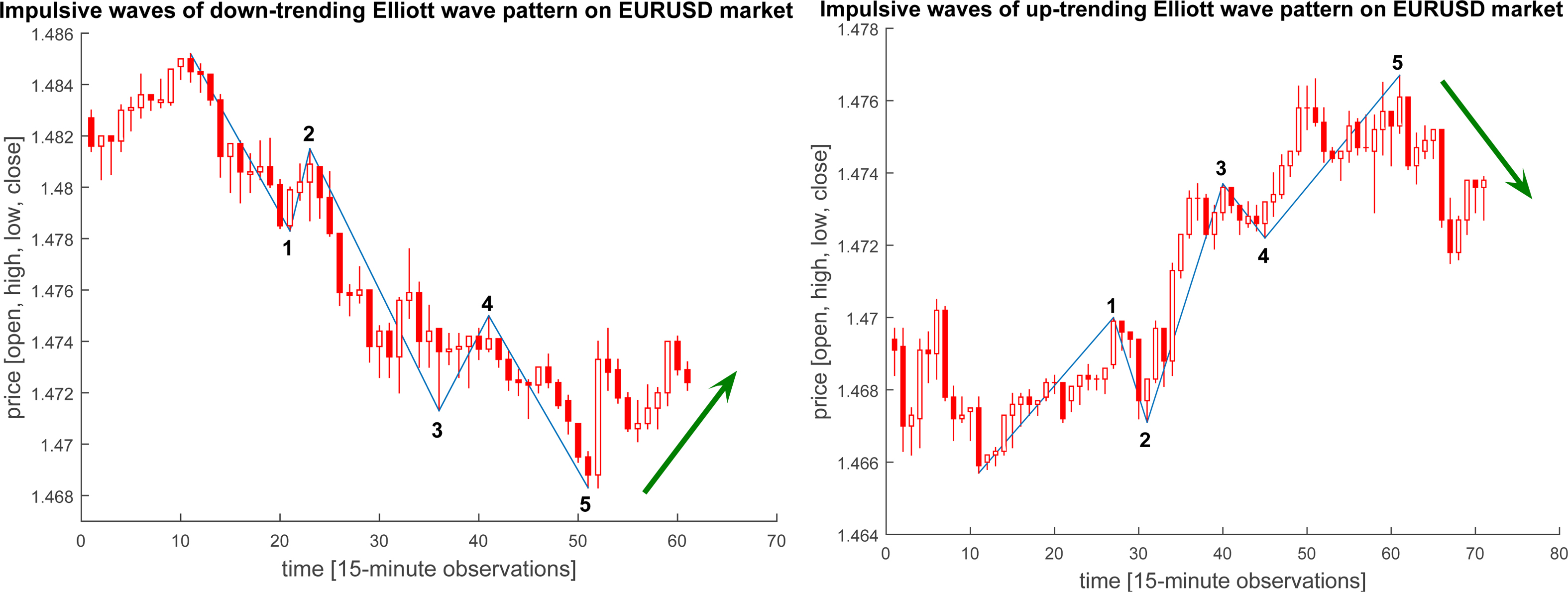

2.3 Filtering the redundancies and overlapped patterns

Rows of the matrix M represent the found EW patterns and columns are the indexes of each of the waves (including the starting point). Some of the rows differs only in few indexes and some of the rows represents patterns which are overlapped. From every group of similar or overlapped patterns it should be saved only one which fits the EW pattern’s conditions the most.

It is computed the cost function of each of the pattern, which is the averaged difference in percentage between found (real) Fibonacci ratio ( $F_{r}$ ) and target level of Fibonacci ratio ( $F_{t}$ ). In cases of applied ranges instead of target levels, the difference outside of the range is taken into account only. The equation of the fitness value is as follows

$\displaystyle cf(W){=}\frac{1}{n}\sum\limits_{i=1}^{n}\begin{cases}\min\left(% \frac{|F_{t_{1}}{-}F_{r}|}{F_{t_{1}}},\ldots,\frac{|F_{t_{m}}-F_{r}|}{F_{t_{m}% }}\right),\\ \quad∼{}\text{rules 2, 4 and 7}.\\ \begin{cases}|F_{l}-F_{r}|/F_{l},\text{ if }F_{r}<F_{l}\\ |F_{h}-F_{r}|/F_{h},\text{ if }F_{r}>F_{h}\\ 0,\text{ if }F_{l}\leqslant F_{r}\leqslant F_{h}\\ \end{cases}\mspace{-20.0mu },\\ \quad∼{}\text{rules 1, 3, 5 and 6}.\end{cases}\mspace{-25.0mu }$ (3)

where $F_{l}$ and $F_{h}$ are the lower and higher border of the defined range respectively. $F_{t_{m}}$ is the $m$ -th defined target level (all of them are checked) of Fibonacci ratio. The patterns are sorted according to their cost value. The best pattern is stored and all similar and overlapping patterns are removed. If the window contains more patterns, which are not overlapped and fits the rules under defined tolerance, algorithm returns all of them.

2.4 Platform description

MATLAB served as a programming language and integrated development environment (IDE) for purposes of implementation and testing of the entire experiment. The source code is provided as an open-source package available for further testing and applications for free [28].

Our experiments were executed on basic PC configuration (4x cpu and 8 GB RAM) with application of parallel environment that is supported by proper design of EW detector.

3. Experimental applications

The first part of the experiment focuses on EW pattern extraction and evaluation of the few basic statistical features of the found patterns. The following part is an evaluation of the impact on the predictable performance of the ML models by application of extracted patterns. The Support Vector Machine (SVM) and Random Decision Forest (RF) were applied algorithms for this trend prediction. The incomplete EW patterns (1-2-3-4 and 1-2-3-4-5) of price values were the input values of these algorithms. The output value of the algorithms were only binary values where 1/0 stands for prediction of up/down-trend (average price of $n$ -future ticks is higher/lower than price of last wave). The value of $n$ is calculated according to the EW rules, where length of forecasted fifth wave should be approximately 1.62 times longer than the first wave (in case of input of 1-2-3-4 waves) and the first corrective wave A should be of similar size as a wave 5 (in case of input of 1-2-3-4-5 waves). There is no guarantee that detected waves (first four or five) will complete the entire EW cycle, which is one of the main reason why the final performance will be decreased. The usefulness of EW pattern application will be compared to prediction based on random selection of the observation as the input value.

3.1 Data acquisition

The stock market data were obtained from public sources. The data is in format of one-minute measurement for MetaTrader platform [29]. It contains the price behavior of GOLD (XAG/USD) from 2011-01-01 to 2015-12-31, SILVER (XAU/USD) from 2011-01-01 to 2015-12-31 and currency pair EURUSD (EUR/USD) from 2005-01-01 to 2015-12-31. These market titles were chosen because the higher amount of trades performed on these titles and free availability of data to study.

Each observation contains open, high, low, close price and traded volume of the commodity. The time series contain more than 2 millions observations in case of GOLD and SILVER and in case of the currency pair, it was more than 4 million observations (ticks). Because of the assumption of possible application of EW’s fractality (ability to be recognized on all of the time-scales), the time series were transformed also into 10-minute, 15-minute and 1-hour time series.

Figure 5.

Graphical interpretation of Optimal Separating Hyperplane between separated observations of SVM classification [35].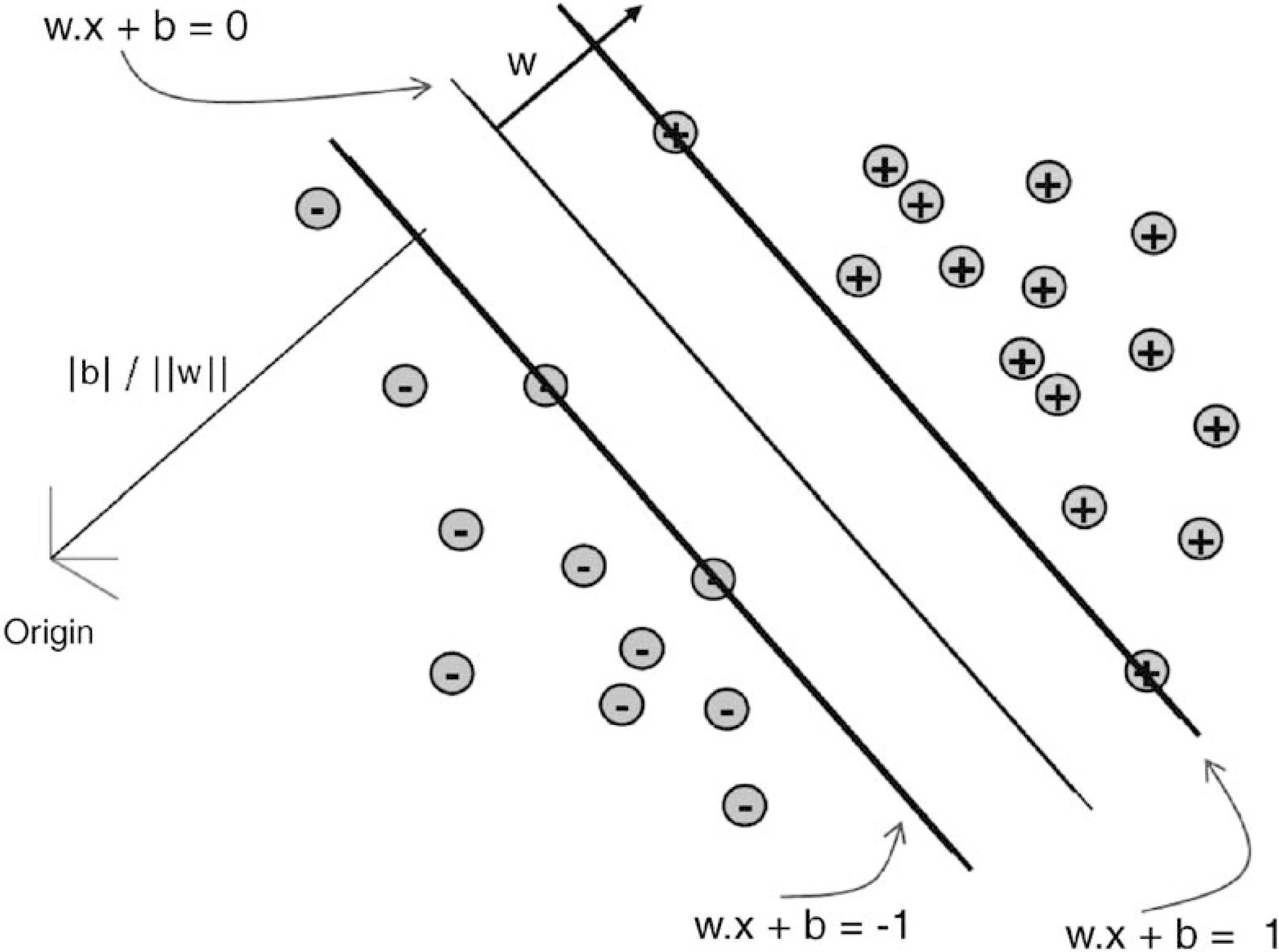

3.2 Binary classification for trend direction prediction

As it was mentioned before, the ML algorithms predict the trend from five or four input values, which represents the prices of wave ends (see in Fig. 4).

The output class represents the following trend direction after the last input wave.

3.2.1 Support Vector Machine

The SVM was introduced by Vapnik in 1995 [30, 31] as a classifier for two-class (binary) problems and from this time it was applied in many studies for stock market prediction [32, 33] or classification [34].

In basic manner, SVM creates mapping for input vector $x$ into the high dimensional feature space where all of the training observations are separable by designed Optimal Separating Hyperplane (OSH). OSH should maximize the distances (so called margins) between the nearest observations and the OSH itself. The observations of one class should be ideally on one of the sides of the space divided by OSH and observations of the second class should be on the opposite side of the OSH. The training observations, which are the closes to the OSH are called as support vectors.

In case of the observations are lineary separable, the solution (OSH) is given by following equation

$Y=\,{\rm sign}\,\left(\sum\limits_{i=1}^{N}y_{i}\alpha_{i}(x\cdot x_{i})+b\right)$ (4)

where $Y$ is the output value, $y_{i}$ is the target value and $\cdot$ represents the product of input vector $x_{i}$ and $N$ support vectors. The $\alpha$ and $b$ represent the parameters of the hyperplane.

In other (non-linear) cases, the SVM applies a kernel transformation function ( $K$ ) which transforms the inputs into high-dimensional feature space, which gives the ability to find suitable OSH.

$Y=\,{\rm sign}\,\left(\sum\limits_{i=1}^{N}y_{i}\alpha_{i}K(x,x_{i})+b\right)$ (5)

There are several known kernel functions which are able to by applied for example polynomial kernel function ( $K(x,x_{i})=(x\cdot x_{i}+1)^{d}$ ), Gaussian radial bases kernel function ( $K(x,x_{i})=\exp(-1/\delta^{2}(x-x_{i})^{2})$ ), etc.

Training of the SVM is equals to solve a linearly constrained quadratic problem (QP) where number of variables is equal to the number of input vectors of the training dataset (see in Fig. 5).

Figure 6.

A decision tree with three input variables (b1, b2 and b3). At each of the root and internal nodes (splits), a statistical measure is applied. The values a, b, c and d are thresholds for splitting. A dataset is split into smaller subsets until the terminal nodes (leaves) return the class labels (A, B and C) [40].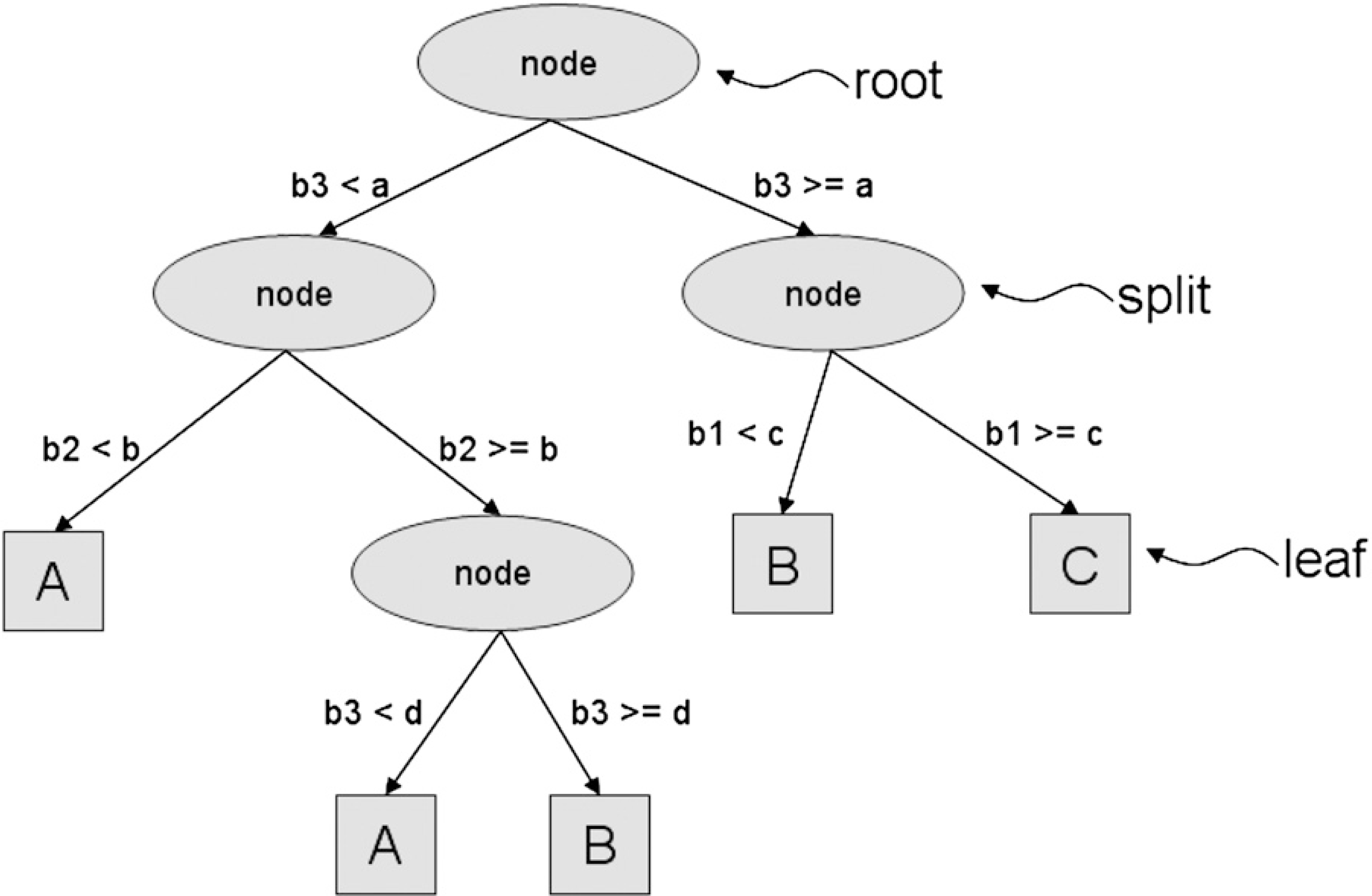

3.2.2 Random Forest

Random Decision Forest is a general title for ensemble based machine learning model which was proposed by Breiman in 2001 [36]. This model was succesfuly applied in many machine learning studies [37, 38]. The core idea of the algorithm is focused on application of an ensemble of CART-like tree classifiers (boosting) and their learning performed on the boosted-aggregated observations (bagging).

The decision tree (DT) is a tree-like structure of conditions with binary output values [39]. These conditions represent the nodes and leaves of the tree and serve as conditions for classification of the observation. Each condition make a single decision on one chosen attribute from the dataset and such an attribute is called splitting criteria. The attribute becomes the splitting criteria, when his information gain value (see Eq. (8)) is the highest on the particular subset of observations. The structure of such tree is depicted in Fig. 6.

$\displaystyle E(S)=-\sum\limits_{j=1}^{n}P(s_{j})\log(P(s_{j}))$ (6) $\displaystyle I(S|A)=\sum\limits_{i}\frac{|S_{i}|}{|S|}\times E(S_{i})$ (7) $\displaystyle G(S|A)=E(S)-I(S|A)$ (8)

Learning of the ensemble of trees means to train the set of trees where each of them obtain different random subset of the observations and different random subset of variables. This process minimizes the correlation between the trees, which increase the robustness of the model and decrease the possible amount of over-fitting. The final classification is derived from voting mechanism where votes from all of the trees are taken into account and final class is assigned to the observation by votes of the majority of the ensemble.

The bootstrapping mechanism comes from statistic and it is also know as random sampling with replacement [41]. This mechanism in context of RF algorithm produces balanced subset of observations for each of the tree. They are trained on resampled observations, which can handle the imbalanced problem or the problem of inability to learn some specific observations.

The other useful feature of RF algorithm is the possibility to compute the importance of the dataset’s variables. The ranking value is derived from averaged value of information gain of the variable across all of the learned trees. This feature was reviewed and applied in many studies [42, 43].

3.3 Hyper-parameter adjustment

During the second phase of the experiment, the trend prediction by ML algorithm, the Grid search optimization was employed to find the near optimal hyper parameter adjustment of the used ML models. The final setting of the parameters is listed in Table 1.

Table 1
Setting of parameters of applied machine learning algorithms

Algorithm	Parameter	Value
RF	Learning algorithm	Decision tree
	Number of trees in ensemble	200
	Applied variables per tree	All
	Applied observations per tree	Random
	Method	Classification
SVM	Optimization method	Sequential minimal
		optimization
	Kernel function	Linear
	C	1.0
	Radius	0.01

Grid search hyper-parameter optimization (GSO) is an optimisation technique frequently applied for fine tuning of the ML model by optimisation of its hyper-parameter values [44]. This process comes through all combinations of parameter values (defined by their ranges) and according to the performance of the classifier, it chooses the best combination of settings.

4. Results

The first part of the experiment was focused on EW pattern detection. The patterns were extracted from windows of length of 1000 observations from time series of ten-minute data and time series of hourly data. The different conditions were applied on the width of the initial fractal. The width of IF was set to 5 observations in case of hourly time series and 9 observations in case 10-minute time series.

All of the EW extractions were proceeded with four level of tolerances (10%, 15%, 20%, 25% for all of the Fibonacci ratios) and only complete EW were taken into account (all of the waves should fit the defined criteria under the given level of tolerance). The hypothesis of this experiment were focused on how the quality and amount of found EW’s depends on adjusted tolerances. The amount of found EW patterns is simply the count of patterns which fulfills the criteria and not over-lap the other selected patterns. EW’s which are inside of some longer EW pattern were not recognized in this experiment.

The median of the EW’s length is also observed. The longer EW is recognized, the easier opportunity is to open the position for a trade in the matter of time. The last statistic that was computed was the Market’s coverage, which simply means the ratio between observations that were members of found pattern to observations without membership to any EW. The higher amount of correctly recognized patterns implies the higher coverage, which leads to higher number of trading opportunities in the market.

Table 2
Description of the quality and amount of founded EW patterns in 10-minute stock market data. The time series described GOLD (G), SILVER (S) and EURUSD (E) markets. For each of the market, there is number of found waves (N) and their average cost value (AC)

Time series		10 min observations (initial fractal width $=$ 9)
Tolerance		10%		15%		20%		25%
		N	AC	N	AC	N	AC	N	AC
Up trend	G	14	5.05%	61	7.39%	120	8.59%	162	9.06%
	S	14	5.01%	55	6.93%	107	8.23%	166	9.09%
	E	44	5.38%	159	6.86%	303	8.41%	411	8.98%
Down trend	G	18	6.11%	69	7.02%	120	8.15%	174	8.82%
	S	13	5.09%	67	7.30%	123	8.55%	169	9.35%
	E	43	4.68%	151	6.69%	305	8.02%	398	8.56%
Avg. length	G	297		228		207		203
	S	281		248		232.5		207
	E	272		203		179		165
Coverage	G	4.19%		15.21%		26.14%		36.10%
	S	3.67%		13.78%		25.33%		34.81%
	E	6.52		19.54		34.72		43.03%

Tables 2 and 3 describe the numbers and quality of found waves and other simple statistic according to the set level of tolerance.

Table 3

Description of the quality and amount of founded EW patterns in 10-minute stock market data. The time series described GOLD (G), SILVER (S) and EURUSD (E) markets. For each of the market, there is number of waves (N) and their average cost value (AC)

Time series		Hourly observations (initial fractal width $=$ 5)
Tolerance		10%		15%		20%		25%
		N	AC	N	AC	N	AC	N	AC
Up trend	G	5	6.31%	17	7.65%	29	7.06%	41	7.84%
	S	5	3.37%	16	4.75%	27	6.33%	31	6.96%
	E	7	5.59%	25	7.34%	43	8.12%	55	8.24%
Down trend	G	4	4.97%	10	5.51%	28	8.77%	39	9.46%
	S	5	7.50%	20	8.27%	31	8.24%	50	9.67%
	E	9	4.78%	30	7.01%	49	8.01%	78	9.06%
Avg. length	G	644		266		237		184.5
	S	260		216		199		188
	E	439.5		254		213.5		181
Coverage	G	11.17%		21.44%		35.93%		45.61%
	S	6.19%		23.41%		33.73%		47.27%
	E	10.41%		26.04%		36.48%		46.34%

The number of found patters increased with higher level of tolerance but on the other hand, the higher number of waves obtained lower quality according to their cost function. The average length of found waves also differs with different applied tolerances. Higher number of found patters implied in all of the cases the higher Market’s coverage.

As it was mentioned before the prediction was simple binary classification (two classes for up/down trends). The input values were prices of waves from incompletely recognized EW patterns and the output value should be the continued trend direction (1 $=$ up-trend, 0 $=$ down-trend). Observations contained complete waves which should continue according to the EW rules and incomplete waves which brings some level of the uncertainty into the classifier.

The number of observations for classification differs for each of the market. In case of the GOLD title, there were 840 observations of 4-wave pattern and 699 observation of 5-wave pattern and in case of the SILVER title, there were 772 observations of 4-wave pattern and 642 observation of 5-wave pattern. Because the EURUSD time set contained the longest observed time-range (more than 4 millions of observations represents 10-year’s data) the number of incomplete patterns was higher. The number of EURUSD’s 4-wave patterns was 1738 and 1464 5-wave patterns.

The cross-validation method [45] was applied for testing of classification performance and the results covers calculated values of accuracy, precision, recall, specificity and basic f-score (see in Table 4).

Table 4

Performance of binary classification for trend predictions, the metrics like accuracy, recall, specificity, precision and f-score are sorted line by line for each of the market title (Gold (G), Silver (S), Eurusd (E))

	(1-2-3-4) waves input			(1-2-3-4-5) waves input
	EW, RF	EW, SVM	Random	EW, RF	EW, SVM	Random
G	52.26%	54.4%	50.29%	64.89%	68.06%	50.14%
	45.05%	55.33%	35.99%	67.66%	69.05%	40.56%
	59.42%	53.6%	63.17%	62.22%	67.15%	64.7%
	49.93%	51.41%	47.54%	62.71%	66.24%	50.44%
	46.86%	53.13%	40.84%	65.06%	65.51%	43.24%
S	48.18%	54.93%	50.29%	67.5%	71.09%	43.44%
	41.95%	53.11%	42.79%	69.35%	74.47%	26.52%
	53.51%	56.44%	58.93%	65.74%	67.9%	69.52%
	43.47%	50.86%	48.82%	67.54%	70.67%	26.69%
	42.56%	51.79%	44.57%	68.28%	72.36%	26.58%
E	55.39%	53.72%	53.29%	66.99%	70.07%	46.71%
	40.3%	55.76%	56.88%	57.62%	68.69%	47.38%
	67.46%	52.17%	50.34%	74.97%	71.24%	46.91%
	49.26%	47.86%	51.43%	66.15%	66.85%	44.93%
	44.11%	51.44%	53.89%	61.50%	67.68%	45.92%

The results between SVM and RF algorithms obtained minimal differences and there is no motivation to compare their performance. The more interesting comparison is the increase of the performance between the application of randomly selected observations (with similar distances as EW’s patterns) and application of extracted EW patterns. As we can see, when the all of the impulsive waves were detected, the trend direction was easier to predict. On the other hand, the incomplete impulsive wave pattern (1-2-3-4) had no difference in progress from the random price picks.

5. Discussion

The Elliott Wave theory was considered as a main idea of this paper, because even if the original idea of the repetitive waved behavior is older, it is still possible to find an occurrence of such a pattern in the price progress. This was the main motivation for the development of the algorithm for EW’s pattern detection.

The pattern matching is driven by the fundamental knowledge based on Fibonacci ratio sequences described in previous studies. The possibility of pattern matching is extended by ability of adjustable tolerance for each of the Fibonacci ratios of the EW’s pattern. It leads to higher amount of found patterns, higher coverage of the market data and also higher control of the trading strategy.

The advantages of the presented algorithm is its simplicity, possibility of running in parallel environment, adjustable tolerances which are able to handle even higher amount of noise interference and no dependence on the length of the time set, that causes the possible finding of EW patterns in all the possible scales and sizes. As a disadvantage, it is considered the inability of self-optimization on a given time set, because the default version of the algorithm does not cover any learning ability. This requirement is possible to fulfill by extension of evolutionary based optimization algorithm, which will optimize the tolerances based on the given criteria. This step will be considered in our future work.

The detected EW patterns worked as a valuable tool for the price progress forecasting, however it was tested only on very specific stock market price titles. Each market title preserves different behavior and the level of fluctuation, that affects the possibility and quality of finding of the EW patterns. Because these conditions vary from title to tile and also across the observed time, the another future study should be aimed on the measurement of relevancy between temporal statistical features and found EW patterns.

6. Conclusions

This paper covers the design, implementation and testing of the algorithm for EW pattern detection. The available literature providing the theory about fundamental features of EW patterns was considered in its development. The open-source package for further research is a result brought by first part of this study.

The second part of this study is focused on application of the developed algorithm. The EW patterns are extracted from three different stock market titles. Different adjustments of the algorithm are compared by quality, length and amount of found waves.

Further the impulsive waves were applied for the trend-prediction. This was compared with randomly selected input waves. The application of complete impulse waves (1-2-3-4-5) implied higher performance than the input based on incomplete impulse waves (1-2-3-4).

Although the conditions of the experiment are not entirely the same from previous studies of the trend-predictions, the results are very comparable which makes the Elliott wave theory still attractive and applicable in this field of interest.

Footnotes

Acknowledgments

This research was conducted within the Students Grant Competition project reg. no. SP2016/175, the framework of the Project TUCENET Sustainable Development of Centre ENET LO1404, supported by Grant SGS 2018/177 of VSB-Technical University of Ostrava; and by The Ministry of Education, Youth and Sports from the National Programme of Sustainability (NPU II) project “IT4Innovations excellence in science – LQ1602”. We also wanted to acknowledge the COMPSE 2016, First EAI International Conference on Computer and Engineering, Penang, Malaysia, November 11–12, 2016.

References

Jensen

. Some anomalous evidence regarding market efficiency. Journal of Financial Economics1978; 6(2-3): 95-101.

Malkiel

. The efficient market hypothesis and its critics. The Journal of Economic Perspectives2003; 17(1): 59-82.

Campbell

. Stock returns and the term structure. Journal of Financial Economics1987; 18(2): 373-399.

Fama

French

. Dividend yields and expected stock returns. Journal of Financial Economics1988; 22(1): 3-25.

Schwert

. Stock returns and real activity: A century of evidence. The Journal of Finance1990; 45(4): 1237-1257.

MacKinlay

. Stock market prices do not follow random walks: Evidence from a simple specification test. Review of Financial Studies1988; 1(1): 41-66.

Rout

Dash

. Forecasting foreign exchange rates using hybrid functional link RBF neural network and Levenberg-Marquardt learning algorithm. Intelligent Decision Technologies2016; 10(3): 299-313.

Yuan

Gao

. Risk decision-making based on Mahalanobis-Taguchi system and grey cumulative prospect theory for enterprise information investment. Intelligent Decision Technologies2016; 10(1): 49-58.

Chen

Ribeiro

. Towards tangible benefits of corporate failure prediction with business sector: A comparative study. Intelligent Decision Technologies; (Preprint): 1-12.

10.

Huang

Nakamori

Wang

. Forecasting stock market movement direction with support vector machine. Computers & Operations Research2005; 32(10): 2513-2522. Applications of Neural Networks.

11.

Atsalakis

Valavanis

. Forecasting stock market short-term trends using a neuro-fuzzy based methodology. Expert Systems with Applications2009; 36(7): 10696-10707.

12.

Choudhry

Garg

. A hybrid machine learning system for stock market forecasting. World Academy of Science, Engineering and Technology2008; 39(3): 315-318.

13.

Meysenburg

Hoelting

McElvain

Foster

. How random generator quality impacts genetic algorithm performance. Proceedings of the 4th Annual Conference on Genetic and Evolutionary Computation, Morgan Kaufmann Publishers Inc.2002; 480-487.

14.

Marmolejo

Rodriguez

. Fat tail model for simulating test systems in multiperiod unit commitment. Mathematical Problems in Engineering, 2015.

15.

Matsumoto

Nishimura

. Mersenne twister: A 623-dimensionally equidistributed uniform pseudo-random number generator. ACM Transactions on Modeling and Computer Simulation (TOMACS)1998; 8(1): 3-30.

16.

Soni

. Applications of ANNs in stock market prediction: A survey. International Journal of Computer Science & Engineering Technology2011; 2(3): 71-83.

17.

Atsalakis

Valavanis

. Surveying stock market forecasting techniques – part II: Soft computing methods. Expert Systems with Applications2009; 36(3): 5932-5941.

18.

Yoo

Kim

Jan

. Machine learning techniques and use of event information for stock market prediction: A survey and evaluation. Computational Intelligence for Modelling, Control and Automation, International Conference on Intelligent Agents, Web Technologies and Internet Commerce, International Conference on, IEEE2005; 2: 835-841.

19.

Enke

Thawornwong

. The use of data mining and neural networks for forecasting stock market returns. Expert Systems with Applications2005; 29(4): 927-940.

20.

Elliott

. Nature’s law – the secret of the universe. New York: 63 Wall St, Elliott RN, (ed). 1946, 64 p. Science Education1947; 31(1): 44-44.

21.

Volna

Kotyrba

Jarusek

. Multi-classifier based on Elliott wave’s recognition. Computers & Mathematics with Applications2013; 66(2): 213-225.

22.

Frost

Prechter

. Elliott wave principle: Key to market behavior. Elliott Wave International, 2005.

23.

Dash

Patil

. An Exploratory Study of Elliott Wave Theory in Indian Stock Markets. Available at SSRN 1412733, 2009.

24.

Atsalakis

Dimitrakakis

Zopounidis

. Elliott Wave Theory and neuro-fuzzy systems, in stock market prediction: The WASP system. Expert Systems with Applications2011; 38(8): 9196-9206.

25.

Poser

. Applying Elliot Wave theory profitably. vol. 169. John Wiley & Sons 2003.

26.

Prechter

. Trading the Elliott Waves: Winning Strategies for Timing Entry & Exit Moves. Marketplace Books 2003.

27.

Williams

Gregory-Williams

. Trading Chaos. John Wiley & Sons 1995.

28.

Vantuch

. EW detector package, 2016. Available from: https://bitbucket.org/tomas_vantuch/ew_detector.

29.

FXDD. MetaTrader 1-Minute Data, 2016. Available from: http://www.fxdd.com/us/en/forex-resources/forex-trading-tools/metatrader-1-minute-data.

30.

Cortes

Vapnik

. Support-vector networks. Machine Learning1995; 20(3): 273-297.

31.

Vapnik

. The nature of statistical learning theory. Springer Science & Business Media1995.

32.

Kim

. Financial time series forecasting using support vector machines. Neurocomputing2003; 55(1): 307-319.

33.

Mukherjee

Osuna

Girosi

. Nonlinear prediction of chaotic time series using support vector machines. Neural Networks for Signal Processing [1997] VII. Proceedings of the 1997 IEEE Workshop, IEEE1997; 511-520.

34.

Shin

Lee

Kim

. An application of support vector machines in bankruptcy prediction model. Expert Systems with Applications2005; 28(1): 127-135.

35.

Caldas

Soibelman

. Automating hierarchical document classification for construction management information systems. Automation in Construction2003; 12(4): 395-406.

36.

Breiman

. Random forests. Machine Learning2001; 45(1): 5-32.

37.

Svetnik

Liaw

Tong

Culberson

Sheridan

Feuston

. Random forest: A classification and regression tool for compound classification and QSAR modeling. Journal of Chemical Information and Computer Sciences2003; 43(6): 1947-1958.

38.

Prinzie

Van den Poel

. Random forests for multiclass classification: Random multinomial logit. Expert Systems with Applications2008; 34(3): 1721-1732.

39.

Quinlan

. C4.5: Programs for Machine Learning. San Francisco, CA, USA: Morgan Kaufmann Publishers Inc.1993.

40.

Chan

JCW

Paelinckx

. Evaluation of Random Forest and Adaboost tree-based ensemble classification and spectral band selection for ecotope mapping using airborne hyperspectral imagery. Remote Sensing of Environment2008; 112(6): 2999-3011.

41.

Efron

Tibshirani

. An introduction to the bootstrap. CRC Press 1994.

42.

Louppe

Wehenkel

Sutera

Geurts

. Understanding variable importances in forests of randomized trees. Advances in Neural Information Processing Systems2013; 431-439.

43.

Chen

Lin

. Combining SVMs with various feature selection strategies. Feature Extraction: Foundations and Applications. Berlin, Heidelberg: Springer Berlin Heidelberg2006; 315-324.

44.

Bergstra

Bengio

. Random search for hyper-parameter optimization. Journal of Machine Learning Research2012; 13(Feb): 281-305.

45.

Kohavi

, et al. A study of cross-validation and bootstrap for accuracy estimation and model selection. IJCAI1995; 14: 1137-1145.

An algorithm for Elliott Waves pattern detection

Abstract

Keywords

1. Introduction

2.2 Pattern selection

3. Experimental applications

3.1 Data acquisition

3.2.1 Support Vector Machine

Table 1 Setting of parameters of applied machine learning algorithms

Table 2 Description of the quality and amount of founded EW patterns in 10-minute stock market data. The time series described GOLD (G), SILVER (S) and EURUSD (E) markets. For each of the market, there is number of found waves (N) and their average cost value (AC)

6. Conclusions

Footnotes

Acknowledgments

References

Table 1
Setting of parameters of applied machine learning algorithms

Table 2
Description of the quality and amount of founded EW patterns in 10-minute stock market data. The time series described GOLD (G), SILVER (S) and EURUSD (E) markets. For each of the market, there is number of found waves (N) and their average cost value (AC)