A discrete gravitational search algorithm for solving the cell formation problem

Abstract

Nowadays, the cellular manufacturing system is thriving into the industrial field due to the higher provided profits and quality of products. Moreover, the manufacturing cell formation problem is considered as the most studied implementation of the cellular manufacturing system. Therefore, a novel gravitational Search Algorithm was introduced and applied to the cell formation problem in this paper. According to the obtained results, the novel gravitational Search Algorithm provides good quality solutions with a reasonable computational time. In the original discrete Gravitational Search Algorithm the exploration strategy was performed by means of a mutation operator applied several times to a solution. To decrease the complexity of the algorithm and the computational time a crossover operator; equivalent to the application of the mutation operator for a number of times; is presented. A modified Local Search algorithm is performed to seek more extensively the solution space. The performance of the novel Gravitational Search Algorithm adaptation was evaluated on a set of 35 benchmarks from the literature. According to the obtained results and to the comparative study, the novel Gravitational Search Algorithm is considered as one of the best algorithms.

Keywords

Cell formation problem gravitational search algorithm local search

1. Introduction

Group technology GT is a concept which had emerged in the late 1950s; it had been first introduced by Mitrofanov and adopted for the first time by the ford Motor Company in the 1970s. Since then GT has been widely applied in the industrial field due to its greater impact on increasing the productivity, quality and also due to its capabilities to improve the manufacturing costs and to decrease the lead time [1].

Application of the GT concept which is known as cellular manufacturing is based on the principle that similar things should be manufactured similarly. One of the most used ways to bring the cellular manufacturing philosophy to bear is called the cell formation problem CFP. The CFP takes its origins from the works performed by the pioneers of the GT such as Flanders (1924), Mitrofanov (1959), Burbidge (1963), Petrov (1966), Ivanov (1968), Durie (1970), Edwards (1971), Grayson (1971), and Gallagher and Knight (1973) and others according to the reference [2].

Given a system within a company, constituted by a set of machines and a set of parts. The CFP consists of dividing the system into subsystems, named cells, in such a manner that the inter-cell movements are decreased and the intra-cell movements are increased. This can be done by grouping parts into families and assign them to groups of machines.

To the best of our knowledge [1, 3, 4, 5], the methods used to solve the cell formation problem can be divided into the following five categories:

1.
Cluster analysis.
2.
Graph partitioning approaches.
3.
Mathematical programming methods.
4.
Heuristic and Metaheuristic algorithms.
5.
Artificial intelligence methodologies.

Despite the fact that a great number of exact methods have been applied to motivated sizes of the CFP [6, 7, 8], the CFP is an NP-complete (hard) problem according to Ballakur and steudel [9]. And for this particular reason, a large number of heuristics have been employed to solve the CFP with good solutions in a reasonable computational time.

The purpose of this paper is to introduce a novel extended version of discrete gravitational search algorithm applied to the cell formation problem. The manufacturing system we have employed is represented by a binary product-machine matrix named the incidence matrix. The discrete gravitational search algorithm has a well-balanced mechanism for enhancing exploration and exploitation abilities. Furthermore, its capability to find the good search space regions in the early iterations [10].

The reminder of this paper is organized as follows. In Section 2, the CFP and the mathematical model are introduced. In Section 3, The Gravitational Search Algorithm (GSA) is presented. Further, the main components of our algorithm are detailed and the performance of our approach is shown by means of the 35 well-known benchmarks. The obtained results show that the proposed DGSA reaches the best-known solutions of 31 benchmarks. Our DGSA also outperform the best-known solution of the 33rd benchmark. Finally, both contributions and concluding remarks are presented in Section 6.
2. The mathematical formulation of the Cell Formation Problem

2.1 The Cell Formation Problem

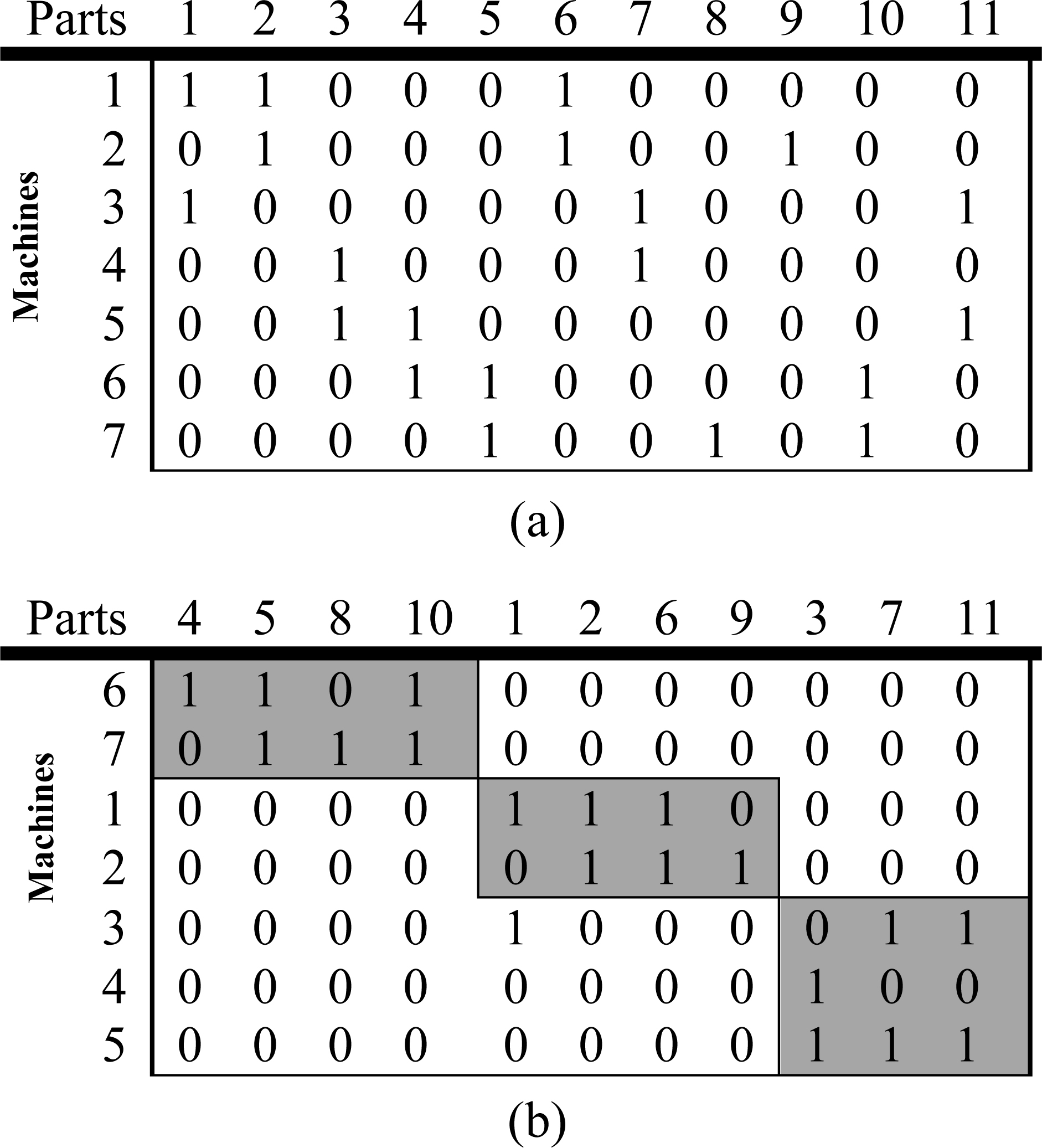
Given a 0-1 machine-part incidence matrix, the main aim of the CFP is to obtain a diagonal block matrix by rearranging the rows and the columns, in such a manner as to construct machine cells and part families. The part families are dispatched to machine cells in the main purpose to optimize the performance measure. In this paper, the Grouping Efficacy was adopted due to its several advantages such as:

a. a.
The ability to incorporate both the with-in cell machine use and the inter-cell movement,
b.
The ability to differentiate between well-struc- tured (with a high with-in cell machine and low inter-cell movement) and ill-structured (with a low with-in cell machine and high inter-cell movement) incidence matrices,
c.
The ability to generate interesting block diagonal matrices,
d.
The simplicity of implementation,
e.
Not requiring a weight factor (weight factor is a measure required in the Grouping Efficiency performance measure).

Figure 1.
An incidence matrix example.

Many performance measures had been cited in literature. A great overview of performance measures can be found in [28, 29]. The Grouping Efficacy is defined as follows:

$\displaystyle\textit{Eff}=\frac{a-a_{1}^{\textit{Out}}}{a+a_{0}^{\textit{In}}}% =\frac{a_{1}^{\textit{In}}}{a+a_{0}^{\textit{In}}}$ (1)

where $a$ is the total number of 1 in the incidence matrix, $a_{0}^{\textit{In}}$ is the number of voids (the number of zeros within a cell), $a_{1}^{\textit{Out}}$ is the number of exceptional elements (the number of $1$ out of all cells), and $a_{1}^{\textit{In}}$ is the number of $1$ within a given cell. An example of a solution of the CFP is shown on Fig. 1, where machines and parts were respectively grouped into cells and families such as each part family were assigned to a cell containing the machines required for the operations.

In Fig. 1b, the Grouping Efficacy is equal to:

$\displaystyle\textit{Eff}=(19-1)/(19+7)=69\%$
2.2 The mathematical model

In this subsection a mathematical model similar to the one presented in [30], is introduced. The mathematical programming model is formulated as bellow:

$\displaystyle\textit{Max}∼{}\textit{Eff}=$ $\displaystyle\frac{\sum\nolimits_{k=1}^{C}{\sum\nolimits_{i=1}^{M}{\sum% \nolimits_{j=1}^{P}{a_{ij}x_{ik}y_{ik}}}}}{a+\sum\nolimits_{k=1}^{C}{\sum% \nolimits_{i=1}^{M}{\sum\nolimits_{j=1}^{P}{(1-a_{ij})x_{ij}y_{ik}}}}}$ (2)

Subject to

$\displaystyle\sum\nolimits_{k=1}^{C}{x_{ik}=1},i=1,\ldots,M$ (3) $\displaystyle\sum\nolimits_{k=1}^{C}{y_{jk}=1},j=1,\ldots,P$ (4) $\displaystyle\sum\nolimits_{i=1}^{M}{x_{ik}\geqslant 1},k=1,\ldots,C$ (5) $\displaystyle\sum\nolimits_{j=1}^{P}{y_{jk}\geqslant 1},k=1,\ldots,C$ (6) $\displaystyle x_{ik}=0\text{ or}1,i=1,\ldots,M,k=1,\ldots,C$ (7) $\displaystyle y_{jk}=0\text{ or}1,j=1,\ldots,P,k=1,\ldots,C$ (8)

where $x_{ik}$ and $y_{ik}$ are two binary variables defined as below:

For each $i=1,\ldots,M,k=1,\ldots,C$

$\displaystyle x_{ik}=\begin{cases}1&\text{if the $i^{\rm th}$ machine belongs % to}\\ &\text{the $k^{\rm th}$ cell}\\ 0&\text{otherwise}\\ \end{cases}$

For each $j=1,\ldots,P,k=1,\ldots,C$

$\displaystyle y_{jk}=\begin{cases}1&\text{if the $j^{\rm th}$ part belongs to}% \\ &\text{the $k^{\rm th}$ cell}\\ 0&\text{otherwise}\\ \end{cases}$

And where

$\displaystyle a_{1}^{\textit{Out}}=a-\sum\nolimits_{k=1}^{C}{\sum\nolimits_{i=% 1}^{M}{\sum\nolimits_{j=1}^{P}\!{a_{ij}x_{ik}y_{jk}}}}$ (9) $\displaystyle a_{0}^{\textit{In}}=\sum\nolimits_{k=1}^{C}{\sum\nolimits_{i=1}^% {M}{\sum\nolimits_{j=1}^{P}{(1{-}a_{ij})x_{ik}y_{jk}}}}$ (10)

$a_{ij}$ denotes the element in the $i^{\rm th}$ row and the $j^{\rm th}$ column of the incidence matrix. The Eqs (3) and (4) ensure that each part and each machine must be assigned to only one cell. The Eqs (5) and (6) guarantee that each cell contains at least one part and one machine. The Eqs (7) and (8) denote that decision variables are binary. In the computational experiments, the number of cells, denoted $k$ , was fixed for each problem to its value in the best-known solution reported in the literature.

3. The gravitational search algorithm

The Gravitational Search Algorithm (GSA) is a population based procedure first proposed in [31] that mimics the Newton’s Law of Gravity and the Law of Motion to solve optimization problem of the form $\mathop{\rm Max}\nolimits_{s\in\mathbb{R}^{n}}fit(s)$ . The value $fit(s)$ measures the fitness of a solution $s=\left({s_{1},\ldots,s_{d},\ldots,s_{n}}\right)\in\mathbb{R}^{n}$ . In the GSA, each solution $s$ corresponds to an agent having four specifications: position $\left({s_{1},\ldots,s_{d},\ldots,s_{n}}\right)$ , inertia mass, active gravitational mass, and passive gravitational mass.

Now assume that $N$ solutions (agents) are available:

$\displaystyle s^{i}=\left({s_{1}^{i},\ldots,s_{d}^{i},\ldots,s_{n}^{i}}\right)% ,i=1,2,\ldots,N.$ (11)

In the context of gravitational motion, good solutions (with higher fitness $fit({s^{i}})$ ) move more slowly than ones having smaller fitness $fit({s^{i}})$ . Hence, agents with smaller fitness navigate around agents with higher fitness. Through the iterations, the gravitational and inertia masse of each agent is regulated. After a while, the solutions will be attracted by the one having the best fit that represents the optimum solution in the search space.

Now at each iteration, all solutions (agents) are modified to mimic the Newton Law of Gravity. At iteration $t$ , we denote the position of solution $i$ by:

$\displaystyle s^{i}(t)=\left({s_{1}^{i}(t),\ldots,s_{d}^{i}(t),\ldots,s_{n}^{i% }(t)}\right),i=1,2,\ldots,N.$ (12)

It is modified according to a velocity vector $v^{i}(t)=\left({v_{1}^{i}(t),\ldots,v_{d}^{i}(t),\ldots,v_{n}^{i}(t)}\right)$ involving an acceleration vector $ac^{i}(t)=\left({ac_{1}^{i}(t),\ldots,ac_{d}^{i}(t),\ldots,ac_{n}^{i}(t)}\right)$ . To determine these vectors, consider the acting force on solution $i$ by another solution $j$ specified as follows:

$\displaystyle F_{d}^{ij}(t)=G(t)\frac{M_{pi}(t)\times M_{aj}(t)}{R_{ij}(t)+\xi% }(s_{d}^{j}(t)-s_{d}^{i}(t)),d=1,2,\ldots,n$ (13)

where $M_{aj}(t)$ represents the active gravitational mass related to agent $j,M_{pi}(t)$ represents the passive gravitational mass related to agent $i,G(t)$ represents the gravitational constant at time $t,\xi$ represents a small constant, and $R_{ij}(t)$ represents the Euclidian distance between the two agents $i$ and $j$ :

$\displaystyle R_{ij}(t)=\left\|{s^{i}(t),s^{j}(t)}\right\|_{2}$ (14)

To include a stochastic characteristic to the GSA, the total force acting on solution (agent) $i$ in a dimension $d$ is determined by a randomly weighted sum of $d^{\rm th}$ components of the forces exerted from other agents:

$\displaystyle\bar{{F}}_{d}^{i}(t)=\sum\limits_{j=1,j\neq i}^{N}{\textit{rand}_% {j}F_{d}^{ij}(t)}$ (15)

where $\textit{rand}_{j}$ denotes a random number in the interval $\left[{0,1}\right].$

Thus, by the Law of Motion, the acceleration of the agent $i$ at a specific time $t$ and at the dimension $d$ , $ac_{d}^{i}(t)$ is specified as follows:

$\displaystyle ac_{d}^{i}(t)=\frac{\bar{{F}}_{i}^{d}(t)}{M_{ii}(t)}$ (16)

where $M_{ii}(t)$ denotes the $i^{\rm th}$ agent inertia mass.

Moreover, the next velocity of the solution (agent) at the next iteration is specified by a fraction of its current velocity to which its current acceleration is added. Therefore, its position and velocity could be defined as follows:

$\displaystyle v_{d}^{i}(t+1)=\textit{rand}_{i}\times v_{d}^{i}(t)+ac_{d}^{i}(t)$ (17) $\displaystyle s_{d}^{i}(t+1)=s_{d}^{i}(t)+v_{d}^{i}(t+1)$ (18)

where $\textit{rand}_{i}$ denotes a uniform random variable in the interval $\left[{0,1}\right].$ This random number is used to give a randomized characteristic to the GSA.

The gravitational constant $G$ is initialized at the beginning of the algorithm, and its value is reduced during the search process to control the search accuracy. In other words, $G$ is a function of the initial value $(G_{0})$ and time $(t):$

$\displaystyle G(t)=G(G_{0},t)$ (19)

The fitness of the updated solution are used to simulate the fact that the best solutions are more attractive and that they induce a larger input on modifying the gravitational and the inertia masses. In implementing the GSA, the three different masses are specified as identical:

$\displaystyle M_{ai}(t)=M_{pi}(t)=M_{ii}(t)=M_{i}(t),$ $\displaystyle\quad i=1,2,\ldots,N$ (20)

Moreover, they are specified as follows:

$\displaystyle m_{i}(t)=\frac{\textit{fit}(s^{i}(t))-\textit{worst}(t)}{\textit% {best}(t)-\textit{worst}(t)}$ (21) $\displaystyle M_{i}(t)=\frac{m_{i}(t)}{\sum\nolimits_{j=1}^{N}{m_{j}(t)}}$ (22)

where $\textit{worst}(t)$ and $\textit{best}(t)$ are defined as follows:

$\displaystyle\textit{best}(t)=\max\limits_{j=1,2,\ldots N}\left\{{\textit{fit}% (s^{j}(t))}\right\}$ (23) $\displaystyle\textit{worst}(t)=\min\limits_{j=1,2,\ldots N}\left\{{\textit{fit% }(s^{j}(t))}\right\}$ (24)

During the early iterations of the procedure, the acting forces on an agent are specified as in relation Eq. (14) to induce an exploration phase of the process to search more extensively the feasible domain. Later during the resolution, the process should move to an exploitation phase as proposed in [31]. Thus in Eq. (14), instead of using all the other solutions to specify the acting force, we use only a set Kbest of the best solution available. Hence in the early stage Kbest includes all the solutions, but its size is reduced during the process to include only the best solutions. Consequently, the Eq. (14) is modified as follows:

$\displaystyle\bar{{F}}_{d}^{i}(t)=\sum\limits_{j\in\textit{Kbest},j\neq i}{% \textit{rand}_{j}F_{d}^{ij}(t)}$ (25)

According to [32] the GSA is one of the swarm intelligence algorithms. The swarm intelligence algorithms, such as particle swarm algorithm, are usually described as a swarm based system leading to emergent behavior specified through interactions between components of the system. Even though, every swarm intelligence algorithms set has its own way to explore and exploit the search space, they all share common principles. Thus, the GSA could be easier to understand for someone used to the particle swarm algorithm.

4. The discrete gravitational search algorithm

In this paper, an approach quite similar to the DGSA proposed in [33] is used to solve the CFP. The chromosomal representation, the initialization of the initial population, the components of the proposed DGSA, and the replacement strategy will be described in detail thereafter.

4.1 The Chromosomal representation

A chromosome $s$ made of $P+M$ genes, is used to represent a solution to the problem. The chromosome $s$ is encoded as a vector of integers. Each integer of the chromosome $s$ takes its value within the $[1,C]$ interval. The chromosome consists of two parts: the parts part, the machines part. Above, Fig. 2 illustrates an example of a chromosome where $s_{j\in\left[{1,P}\right]}$ denotes the cell to which the part $j$ is assigned and where $s_{{}_{i\in\left[{P+1,M+P}\right]}}$ denotes the cell to which the machine $(i-P)$ is assigned.

Figure 2.

The chromosomal representation.

The chromosomal representation of the solution matrix in Fig. 1. above is as follows:

4.2 The generation of the initial population

The initial population contains $I_{\textit{size}}$ individuals ordered incrementally. $I_{\textit{size}}-1$ dissimilar individuals are randomly generated. A solution constructed by combining the-group-and-assign method introduced in [34] and the approach presented in [35], is injected into the population. The set of individuals constituting the current population is denoted Population.

Generation of the initial population
$l:=1$
while $l<I_{\textit{size}}$ do
(Generation of an individual $s^{l}$ )
for $i:=1$ to $P+M$ do
Generated randomly an integer $k\in[{1,C}]$
Assign the $i^{\rm th}$ part or machine to the $k^{\rm th}$ cell
end for
Apply the correction process to $s^{l}$
if $s^{l}\notin\textit{Population}$ then
$s^{l}$ is injected into Population
$l:=l+1$
end if
end while
Construction of the injected solution $s^{I_{\textit{size}}}$
Apply the correction process to $s^{I_{\textit{size}}}$
Inject $s^{I_{\textit{size}}}$ into Population
Order the individuals of Population incrementally

The Construction of the injected solution
Group-and-Assign method: Forming the machine groups
(stage1)
$k:=1$
generate randomly an integer $i\in\left[{1,M/C}\right]$
assign the $i^{\rm th}$ machine to the $k^{\rm th}$ cell
$\textit{memory}:=i$
for $k:=2$ to $C$ do
for $i:=1$ to $M$ do
if $\textit{memory}\neq i$ then
assign the $i^{\rm th}$ machine to the $k^{\rm th}$ cell
end if
end for
end for
(stage2)
for $i:=1$ to $M$ do
if $i\notin ma$ then
$\textit{flow}:=0$
$\textit{Flow}:=0$
$c:=0$
for $k:=1$ to $C$ do
for $j:=1$ to $P$ do
if $a_{ij}==d_{kj}$ then
$\textit{flow}:=\textit{flow}+1$
end if
end for
if $\textit{Flow}<\textit{flow}$ then
$\textit{Flow}:=\textit{flow}$
$c:=k$
end if
end for
assign the $i^{\rm th}$ machine to the $c^{\rm th}$ cell
update the $m a$ set
end if
end for
The Rojas Approach: Forming the part families
for $j:=1$ to $P$ do
$f:=0$
$c:=0$
for $k:=1$ to $C$ do
define $u_{jk},v_{jk},{\displaystyle\frac{u_{jk}}{e+v_{jk}}}$
if ${\displaystyle\frac{u_{jk}}{e+v_{jk}}}>f$ then
$f:={\displaystyle\frac{u_{jk}}{e+v_{jk}}}$
$c:=k$
end if
end for
assign the $j^{\rm th}$ part to the $c^{\rm th}$ cell
end for
apply the correction process

The group-and-assign method is employed to form the machine groups in two stages. The first stage consists of assigning one machine to each cell. The second stage consists of assigning the remaining machines to cells with the aim of maximizing the total part flow within cells.

$D$ is a $C\times P$ matrix. The $D$ matrix indicates the parts proceeded by machines within a given cell. $d_{kj}$ denotes the element in the $k^{\rm th}$ row and the $j^{\rm th}$ column of the $D$ matrix.

For each $k=1,\ldots,C,j=1,\ldots,P$

$d_{kj}=\begin{cases}1&\text{if the $j^{\rm th}$ part is proceeded within}\\ &\text{the $k^{\rm th}$ cell}\\ 0&\text{otherwise}\end{cases}$

The set of assigned machines is denoted $m a$ .

The approach introduced in [35] is used to assign parts to groups of machines. It mainly consists in assigning each part to the cell that maximized the quotient $\frac{u_{jk}}{e+v_{jk}}$ where the variable $u_{jk}$ denotes the number of machines in the $k^{\rm th}$ cell that process the part $j$ , the variable $v_{jk}$ denotes the number of machines within the $k^{\rm th}$ cell that doesn’t process the part $j$ and $e$ denotes the number of machines processing the part $j$ .

The correction process proceeds by assigning at least and at most one part and one machine to empty cells. To accomplish the correction process, empty cells and cells containing more than one machine or one part have to be defined. In our case, an empty cell is a cell that does not contains at least one part or at least one machine. Two matrices serve to identify empty cells and cells containing more than one machine or one part. Those matrices are denoted $H$ and $W$ . $H$ is a $C\times M$ matrix. The $H$ matrix indicates the machines assigned to each cell. $h_{ki}$ denotes the element in the $k^{\rm th}$ row and the $i^{\rm th}$ column of the $H$ matrix.

For each $k=1,\ldots,C,i=1,\ldots,M$

$h_{ki}=\begin{cases}1&\text{if the $j^{\rm th}$ machine is within}\\ &\text{the $k^{\rm th}$ cell}\\ 0&\text{otherwise}\end{cases}$

$W$ is a $C\times P$ matrix. The $W$ matrix indicates the parts assigned to each cell. $w_{kj}$ denotes the element in the $k^{\rm th}$ row and the $j^{\rm th}$ column of the $H$ matrix.

Figure 3.

The proposed DGSA flowchart.

For each $k=1,\ldots,C,j=1,\ldots,P$

$w_{ki}=\begin{cases}1&\text{if the $j^{\rm th}$ part is within the $k^{\rm th}% $ cell}\\ 0&\text{otherwise}\end{cases}$

The set of cells with no part is denoted $e c p$ . The set of the parts of the cells containing more than one part is denoted $n c p$ . $ecp_{0}$ denotes the first element of $e c p$ . $ncp_{0}$ denotes the first element of $n c p$ . Analogically, the set of cells with no machine is denoted $e c m$ . The set of the machines of the cells containing more than one machine is denoted $n c m$ . $ecm_{0}$ denotes the first element of $e c m$ . $ncm_{0}$ denotes the first element of $n c m$ .

The correction process
construct $n c p$ and $e c p$ sets based on $W$
while $ecp\neq\emptyset$ do
assign the part $ncp_{0}$ to the cell $ecp_{0}$
$ncp-\left\{{ncp_{0}}\right\}$
$ecp-\left\{{ecp_{0}}\right\}$
end while
construct $n c m$ and $e c m$ sets based on $H$
while $ecm\neq\emptyset$ do
assign the part $ncm_{0}$ to the cell $ecm_{0}$
$ncm-\left\{{ncm_{0}}\right\}$
$ecm-\left\{{ecm_{0}}\right\}$
end while

4.3 The components of the proposed gravitational search algorithm

The Discrete Gravitational Search algorithm has two main phases: the Dependent Movement Search Operator Phase (DMSOP) and the Independent Movement Operator Phase (IMSOP). The DMSOP is based on a movement operator. The movement operator gets the current position of an agent and its Dependent Movement Length (DML) as input parameters. The movement operator returns a new position in the solution space as output. The DML is the acceleration vector calculated by the Eq. (16). The IMSOP is a modified version of a local search algorithm. Indeed, the independent movement length (IML) calculated by means of the Eq. (17) is added as a stopping criterion. The Fig. 3 shows the DGSA flowchart.

4.3.1 The dependent movement search operator phase for the cell formation problem

The DMSOP consists of iteratively applying a cross- over operator to a solution denoted $s^{l}$ and a solutions within the Kbest set denoted $s^{o\in\left[{I_{\textit{size}}-I_{\textit{best}},I_{\textit{size}}}\right]}$ . The $I_{\textit{best}}$ variable denotes the size of the Kbest set.

The Dependent Movement Search Operator Phase (DMSOP)
generate randomly an integer $l\in\left[{1,I_{\textit{size}}}\right]$
for $o:=I_{\textit{size}}-I_{best}$ to $I_{\textit{size}}$ do
$s^{l}:=s^{l}\times s^{o}$ ( $\times$ denotes the crossover operator )
end for
assign $s^{l}$ to the $l^{\rm th}$ position

Let assume that $s^{l}$ and $s^{\circ}$ are represented as follows:

$\displaystyle\begin{array}[]{cccccccc}s_{1}^{l}&s_{2}^{l}&\ldots&s_{P}^{l}&s_{% P+1}^{l}&s_{P+2}^{l}&\ldots&s_{P+M}^{l}\\ s_{1}^{\circ}&s_{2}^{\circ}&\ldots&s_{P}^{\circ}&s_{P+1}^{\circ}&s_{P+2}^{% \circ}&\ldots&s_{P+M}^{\circ}\end{array}$

The crossover consists of mixing up the elements of $s^{l}$ and $s^{\circ}$ by using the acceleration vector of $s^{\circ}$ . The acceleration vector of $s^{\circ}$ is denoted $ac_{o}$ . The $ac_{o}$ is a $P+M$ vector calculated by means of the Eq. (16). For each element of $ac_{o}$ we calculate $\textit{Diff}=ac_{o}^{r}-ac_{o}^{d}$ where $d\in\left\{{1,2,\ldots,M+P}\right\}$ and $r\in[1,P+M]$ . If $\textit{Diff}\prec 0,s_{d}^{3}=s_{d}^{l}$ otherwise $s_{d}^{3}=s_{d}^{\circ}$ . $s^{3}$ denotes the output solution of the crossover operator.

The output vector of the crossover operator

$\displaystyle s_{1}^{3}\ \ s_{2}^{3}\ \ \ldots\ \ s_{P}^{3}\ \ s_{P+1}^{3}\ \ % s_{P+2}^{3}\ \ \ldots\ \ s_{P+M}^{3}$

The crossover operator
generate an integer $r\in\left[{1,P+M}\right]$
for $d:=1$ to $P+M$ do
calculateDiff
if $\textit{Diff}\prec 0$ then
$s_{d}^{3}=s_{d}^{l}$
else
$s_{d}^{3}=s_{d}^{o}$
end if
end for
Generate a reel number $p_{\textit{imp}}\in\left[{0,1}\right]$
if $p_{\textit{imp}}\succ 0.5$ then
apply the improvement process
end if

The improvement process enhances the part of machines based on the part of parts and vice versa. The improvement process used in this paper is detailed below.

The improvement process
$s^{1}:=s^{0}$
for $i:=1$ to $P$ do
$\textit{maxf}:=0$
$sc:=-1$
for $c:=1$ to $C$ do
$a_{1}^{\textit{Out}}:=0$
$a_{0}^{\textit{In}}:=0$
for $j:=1$ to $M$ then
if $a_{ji}==1$ and $h_{cj}==0$ then
$a_{1}^{\textit{Out}}:=a_{1}^{\textit{Out}}+1$
end if
if $a_{ji}==0$ and $h_{cj}==1$ then
$a_{0}^{\textit{In}}:=a_{0}^{\textit{In}}+1$

end if

end for

\textit{maxf}\prec{\displaystyle\frac{a-a_{1}^{\textit{Out}}}{a+a_{0}^{\textit% {In}}}}

then

\textit{maxf}:={\displaystyle\frac{a-a_{1}^{\textit{Out}}}{a+a_{0}^{\textit{In% }}}}

sc:=c

end if

end for

s_{i}^{1}:=sc

end for

s^{2}:=s^{1}

for

i:=1

M

\textit{maxf}:=0

sc:=-1

for

c:=1

C

a_{1}^{\textit{Out}}:=0

a_{0}^{\textit{In}}:=0

for

j:=1

P

a_{ij}==1

and

w_{ci}==0

then

a_{1}^{\textit{Out}}:=a_{1}^{\textit{Out}}+1

end if

a_{ij}==0

and

w_{ci}==1

then

a_{0}^{\textit{In}}:=a_{0}^{\textit{In}}+1

end if

end for

\textit{maxf}\prec{\displaystyle\frac{a-a_{1}^{\textit{Out}}}{a+a_{0}^{\textit% {In}}}}

then

\textit{maxf}:={\displaystyle\frac{a-a_{1}^{\textit{Out}}}{a+a_{0}^{\textit{In% }}}}

sc:=c

end if

end for

s_{i}^{2}:=sc

end for

s^{3}:=s^{2}

update

H

for

i:=1

P

\textit{maxf}:=0

sc:=-1

for

c:=1

C

a_{1}^{\textit{Out}}:=0

a_{0}^{\textit{In}}:=0

for

j:=1

M

then

a_{ji}==1

and

h_{cj}==0

then

a_{1}^{\textit{Out}}:=a_{1}^{\textit{Out}}+1

end if

a_{ji}==0

and

h_{cj}==1

then

a_{0}^{\textit{In}}:=a_{0}^{\textit{In}}+1

end if

end for

\textit{maxf}\prec{\displaystyle\frac{a-a_{1}^{\textit{Out}}}{a+a_{0}^{\textit% {In}}}}

then

\textit{maxf}:={\displaystyle\frac{a-a_{1}^{\textit{Out}}}{a+a_{0}^{\textit{In% }}}}

sc:=c

end if

end for

s_{i}^{3}:=sc

end for

s^{0}:=\textit{maximum}(s^{1},s^{2},s^{3})

4.3.2 The independent movement search operator phase for the cell formation problem

The Independent Movement Search Operator Phase is a modified local search algorithm. In this paper a Tabu search algorithm with short memory, is used as an IMSOP. The Tabu search algorithm was first introduced by [36] and then extended in [37]. The main purpose of the Tabu search algorithm is to overcome the local optima. The IMSOP starts with a given solution and iteratively seeks for better solutions by applying either the add/drop operator or the swap operator with the probability $p$ in such a way that the moves within the Tabu list are forbidden unless the aspiration criteria are met. This process is continued until the stopping criteria are met. The correction process introduced above had been embedded in the Tabu search algorithm. To use the Tabu search five concepts have to be defined. Those five concepts are: the neighborhood structure, the movement operators, the Tabu list, the aspiration criteria and the stopping criteria.

The Independent Movement Search Operator Phase
choose randomly a solution $s^{s}$
$s^{0}:=s^{s}$
$s^{1}:=s^{s}$
Generate randomly an integer $r\in\left[{1,P+M}\right]$
$\textit{IML}?:=2v_{r}^{s}+100(M+1)$
while $\textit{iter}\leqslant\textit{IML}$ or $\textit{iter}\leqslant\textit{maxit}$ do
$it:=0;$
while $it\leqslant I_{\textit{neighbor}}$ do
if $noT<2$ then
generate randomly a reel number $r\in\left[{0,1}\right]$
if $r\prec 0.5$ then
(add/drop operator)
generate randomly an integer $i\in$
$\left[{1,P+M}\right]$
generate randomly an integer $c\in\left[{1,C}\right]$
$s_{i}^{0}:=c$
apply the improvement process
apply the correction process
if $\textit{fit}(s^{0})\succ\textit{fit}(s^{1})$ then
$s^{1}:=s^{0}$
end if
$s^{0}:=s^{s}$
end if
if $r\prec 0.5$ then
(swap operator)
generate randomly an integer $i\in$
$[1,P+M]$
generate randomly an integer $j\in$
$[{1,P+M}]$
$\textit{temp}:=s_{j}^{0}$
$s_{j}^{0}:=s_{i}^{0}$
$s_{i}^{0}:=\textit{temp}$
apply the improvement process
apply the correction process
if $\textit{fit}(s^{0})\succ\textit{fit}(s^{1})$ then
$s^{1}:=s^{0}$
end if
$s^{0}:=s^{s}$
end if
else
generate randomly a reel number $r\in[{0,1}]$
if $r\prec 0.5$ then
(add/drop operator)
choose randomly $(i,c)\in poT$
$s_{i}^{0}:=c$
apply the improvement process
apply the correction process
if $\textit{fit}(s^{0})\succ\textit{fit}(s^{1})$ then

s^{1}:=s^{0}

end if

update

n o T

update

p o T

t_{cj}:=t_{cj}+10

s^{0}:=s^{s}

end if

r\prec 0.5

then

(swap operator)

choose randomly

(i,c)\in poT

generate randomly an integer

j\in

[{1,P+M}]

\textit{temp}:=s_{j}^{0}

s_{j}^{0}:=s_{i}^{0}

s_{i}^{0}:=\textit{temp}

apply the improvement process

apply the correction process

\textit{fit}(s^{0})\succ\textit{fit}(s^{1})

then

s^{1}:=s^{0}

end if

update

n o T

update

p o T

t_{cj}:=t_{cj}+10

t_{\textit{temp},i}:=t_{\textit{temp},i}+10

s^{0}:=s^{s}

end if

\textit{iter}:=\textit{iter}+1;

end while

it:=it+1

s^{0}:=s^{1}

s^{s}:=s^{1}

end while

A solution is $s^{1}$ a neighbor of $s^{2}$ , if $s_{d}^{1}=s_{d}^{2},d\in[1,P+M]$ except for at least one dimension and at most for two dimensions. The neighborhood size is denoted $I_{\textit{neighbor}}$ . In our paper, $I_{\textit{neighbor}}$ is fixed at $M/4$ . The operators used to move toward the search space are the add/drop operator and swap operator. The add/drop operator randomly takes an element and modifies it. The swap operator exchanges two elements of a given solution. The Tabu list stores the tabu movements. In our case we used a $C\times(P+M)$ matrix denoted $T$ as a tabu list. $t_{ij}$ denotes the $i^{\rm th}$ row and the $j^{\rm th}$ column of the matrix $T$ . If a machine or a part $j$ is assigned to the $i^{\rm th}$ cell $t_{ij}$ increases. In our case, we consider a short-term memory tabu search thereby the value 10 is added to $t_{ij}$ . Consequently, movements are made tabu for 10 iterations if aspiration criteria are not met. The aspiration criteria are the circumstances in which the tabu list is ignored. The tabu list is ignored if the number of none tabu movements is lower than 2. the number of none tabu movements is denoted $n o T$ . $p o T$ is the set of none tabu positions. A none tabu position is $(i,c)$ couple with $i\in[1,P+M]$ and $c\in[1,C]$ . The Tabu search stops when it reaches IML or maxit. maxit denotes the number of maximum iterations and IML denotes the independent movement search of a starting solution denoted $s^{s}$ .

4.3.3 The replacement strategy for the Cell Formation Problem

In this paper, we used an uncommon replacement strategy. The resulting solution of DMSOP replaces a randomly chosen individual in the population. Moreover, the resulting solution of DMSOP is whether a black box or not. A black box solution is a solution which takes the fitness of the individual it replaces. The resulting solution of IMSOP is injected into the population according a replacement quite similar the elitist replacement. The replacement strategy is detailed below.

The replacement strategy
Generate randomly an integer $r\in\left[{1,I_{\textit{size}}}\right]$
$\textit{Population}(r):=s^{e}$
Generate randomly a reel number $\textit{rand}\in\left[{0,1}\right]$
if $\textit{rand}\prec 0.5$ then
$s^{r}$ is a black box
end if
$j:=-1$
for $i:=1$ to $I_{\textit{size}}$ do
if $\textit{fit}(s^{b})\prec\textit{fit}(s^{f})$ then
$j:=I_{\textit{size}}$
$\textit{Population}(j):=s^{f}$
break
end if
if $\textit{fit}(s^{i})\prec\textit{fit}(s^{f})$ and $\textit{fit}(s^{i+1})\succ\textit{fit}(s^{f})$ then
$j:=i$
$\textit{Population}(j):=s^{f}$
break
end if
end for
if $j==-1$ then
$j:=0$
$\textit{Population}(j):=s^{f}$
end if

Table 1
The relevant parameters of DGSA

Parameter	Value
The size of the population	3 $M$
The number of iterations	500
The size of the set	$3M-1$
The value of the initial G	100

Table 2

Computational results

				DGSA
Problem	M	P	C	Worst Eff	Best Eff	Average Eff	Time (second)	Best known Eff	Gap (%)
P1	5	7	2	82.35	82.35	82.35	0.0219	82.35	0
P2	5	7	2	69.57	69.57	69.57	0.0156	69.57	0
P3	5	18	2	79.59	79.59	79.59	0.0124	79.59	0
P4	6	8	2	76.92	76.92	76.92	0.0141	76.92	0
P5	7	11	5	60.87	60.87	60.87	0.0937	60.87	0
P6	7	11	4	70.83	70.83	70.83	0.0234	70.83	0
P7	8	12	4	69.44	69.44	69.44	0.0266	69.44	0
P8	8	20	3	85.25	85.25	85.25	0.0188	85.25	0
P9	8	20	2	58.72	58.72	58.72	0.039	58.72	0
P10	10	10	5	75	75	75	0.0577	75	0
P11	10	15	3	92	92	92	0.0236	92	0
P12	14	24	7	72.06	72.06	72.06	0.3263	72.06	0
P13	14	24	7	71.83	71.83	71.83	0.3766	71.83	0
P14	16	24	8	53.26	53.26	53.26	4.1425	53.26	0
P15	16	30	6	69.53	69.53	69.53	0.915	69.53	0
P16	16	43	8	57.53	57.53	57.53	10.6387	57.53	0
P17	18	24	9	57.73	57.73	57.73	3.6019	57.73	0
P18	20	20	5	43.06	43.17	43.109	164.3702	43.45	0.64
P19	20	23	7	50.81	50.81	50.81	4.3093	50.81	0
P20	20	35	5	77.91	77.91	77.91	1.6562	77.91	0
P21	20	35	5	57.14	57.14	57.14	280.6444	57.98	1.45
P22	24	40	7	100	100	100	1.1683	100	0
P23	24	40	7	85.11	85.11	85.11	1.3688	85.11	0
P24	24	40	7	73.51	73.51	73.51	1.3756	73.51	0
P25	24	40	11	53.29	53.29	53.29	53.4848	53.29	0
P26	24	40	12	48.95	48.95	48.95	393.5611	48.95	0
P27	24	40	12	46.58	46.58	46.58	957.4588	47.26	1.44
P28	27	27	5	54.82	54.82	54.82	11.047	54.82	0
P29	28	46	10	47.08	47.08	47.08	584.1145	47.08	0
P30	30	41	14	63.31	63.31	63.31	790.244	63.31	0
P31	30	50	13	59.77	59.77	59.77	2033.4975	60.12	0.58
P32	30	50	14	50.83	50.83	50.83	792.9925	50.83	0
P33	36	90	17	47.9	48.01	47.97	1128.0133	47.75	$-$ 0.5
P34	37	53	3	60.64	60.64	60.64	399.5972	60.64	0
P35	40	100	10	84.03	84.03	84.03	42.2884	84.03	0

5. The computational results

In this section, a statistical study is performed to define the parameter values of the DGSA. Based on these parameter values, a comparative study is accomplished to evaluate the performance of the proposed algorithm.

Figure 4.

The Population size and the gap variation graph.

Figure 5.

The probability of improving process and the gap variation graph.

Figure 6.

The number of required iterations and the gap variation graph.

The measure used to evaluate the algorithm performance is called gap. The gap is a measure which represents the difference between the obtained results average denoted A and the best known solution denoted B for a given instance. The gap is calculated as follows:

$\displaystyle gap(\%)=\frac{B-A}{B}\times 100$ (26)

In the DGSA introduced by [33] the Kbest set size and the gravitational constant parameters were defined as relevant parameters so we kept the same strategies to determine their values. To define the other relevant parameters of the proposed DGSA, a statistical study was performed. Based on experiments, we noticed that the value of the gap variable depends on the values of $p_{\textit{imp}}$ , $I_{\textit{size}}$ and $q_{\textit{iteration}}$ (the number of required iterations) variables. To verify the relevance of mentioned parameters, we used the multiple regression method. The multiple regression is a statistical process that defines the relationships among variables by means of the regression model. In our model the dependent variable is the gap variable. The independent variables in the model are $p_{\textit{imp}}$ , $I_{\textit{size}}$ and $q_{\textit{iteration}}$ .

Ten different executions of the DGSA with different values of the independent variables were performed. We randomly picked up the $p_{\textit{imp}}$ , $I_{\textit{size}}$ and $q_{\textit{iteration}}$ values for the 35 problems. The statistical study shows that the relation between the dependent variable and independent variables is statically significant. The Fig. 4 shows that the gap variable value is almost constant even if $I_{\textit{size}}$ varies. Therefore $I_{\textit{size}}$ is not considered as a regression model variable. Unlike the Fig. 4, the Figs 5 and 6 confirm that the variations of $p_{\textit{imp}}$ and $q_{\textit{iteration}}$ influence the gap value. Furthermore, the statistical study demonstrates that only 74.49% of the gap variation is explained by the variations of $p_{\textit{imp}}$ and $q_{\textit{iteration}}$ .

The regression model is defined as bellow:

$\displaystyle gap=0.5329-0.152p_{\textit{imp}}+0.0012q_{\textit{iteration}}$ (27)

The Multiple Regression process uses two statistical tests to demonstrate the significance of variables. The statistical tests are named Fisher and Student tests.

The fisher and student tests shows that $p_{\textit{imp}}$ and $I_{\textit{size}}$ are significance variables. Therefore, inasmuch as the value of the $p_{\textit{imp}}$ is known, we can use the Eq. (26) to predict the value of $q_{\textit{iteration}}$ and inversely. The parameters which play a major role in the performance of the method, are provided in Table 1.

After adjusting the parameters, the proposed DGSA was tested on a set of 35 benchmarks from literature. Those 35 benchmarks are used in a great number of works. The size of benchmarks and the best cell size were reported in Table 2. The proposed heuristic was coded in JAVA language, and was run on a personal computer with an intel Core i5-2540M 2.60 GHz processor. For each instance, the algorithm was run 10 times.

Moreover, the gap, the average CPU time, the best, the worst and the average efficacy were also reported in Table 2. The references of the benchmark instances and the best-known solutions could be found in [55] and [56]. The best obtained results were compared to the best known solutions. The comparison in Table 2 shows that our DGSA outperforms the best known solution for the 33th problem and didn’t reach the best known solution for four problems (P18, P21, P27 and P31). The appendix gives the block diagonal matrices for the best solutions found by the DGSA for all 35 problems.

The obtained results by the DGSA were also compared to the results reported for the cell formation problem using the following methods:

11. 1.

ZODIAC method proposed in [38].

GRAFICS method proposed in [39].

WFA – water flow algorithm proposed in [40].

EA – evolutionary algorithm proposed in [41].

GRASP proposed in [42].

GATSP genetic algorithm proposed in [43].

HGA – hybrid genetic algorithm proposed in [44].

GA – genetic algorithm proposed in [45].

HGDE – differential evolution algorithm proposed in [46].

10.

ACO – ant colony optimization proposed in [47].

11.

HGGA – grouping genetic algorithm proposed in [48].

12.

SACF – simulated annealing algorithm proposed in [49].

13.

GAA – genetic algorithm approach proposed in [50].

Table 3

Comparative study

Problems	ZODIAC	GRAFICS	WFA	EA	GRASP	GATSP	HGA	GA	HGDE	ACO	HGGA	SACF	GAA	SCF-BMCF	EnGGA	SA	$\textit{SA}_{\textit{YLL}}$	The	The
																		proposed	best
																		method	solution
P1	73.68	73.68	73.68	73.68	73.68	–	73.68	–	82.35	82.35	82.35	–	–	–	82.35	75.00	82.35	82.35	82.35
P2	56.22	60.87	62.50	62.50	62.50	68.00	69.57	62.50	69.57	69.57	69.57	69.57	69.57	69.57	69.57	69.57	69.57	69.57	69.57
P3	–	–	79.59	79.59	79.59	77.36	79.59	77.36	79.59	79.59	79.59	79.59	79.59	79.59	79.59	80.85 ${}^{\rm a}$	79.59	79.59	79.59
P4	–	–	76.92	76.92	76.92	76.92	76.92	76.92	76.92	76.92	76.92	76.92	76.92	76.92	76.92	79.17	76.92	76.92	76.92
P5	39.13	53.12	53.13	53.13	53.13	46.88	58.62	50.00	60.87	60.87	60.87	60.87	60.87	60.87	60.87	60.00	60.87	60.87	60.87
P6	–	–	70.37	70.37	70.37	70.37	70.37	70.37	70.83	70.83	70.83	70.83	70.83	70.83	70.83	70.83	70.83	70.83	70.83
P7	68.30	68.30	68.29	68.29	68.29	–	68.30	–	69.44	69.44	69.44	–	–	–	69.44	69.44	69.44	69.44	69.44
P8	85.25	85.25	85.25	85.25	85.25	85.25	85.25	85.25	85.25	85.25	85.25	85.25	85.25	85.25	85.25	85.25	85.25	85.25	85.25
P9	58.33	58.13	58.72	58.72	58.72	58.33	58.72	55.91	58.72	58.72	58.72	58.41	58.72	58.72	58.72	58.72	58.72	58.72	58.72
P10	70.59	70.59	70.59	70.59	70.59	70.59	70.59	72.79	75.00	75.00	75.00	75.00	75.00	75.00	–	75.00	75.00	75.00	75.00
P11	92.00	92.00	92.00	92.00	92.00	92.00	92.00	92.00	92.00	92.00	92.00	92.00	92.00	92.00	–	92.00	92.00	92.00	92.00
P12	64.36	64.36	69.86	69.86	69.86	–	70.83	–	72.06	72.06	72.06	–	–	–	–	74.24 ${}^{\rm a}$	72.06	72.06	72.06
P13	65.55	65.55	69.33	69.33	69.33	67.44	70.51	63.48	71.83	71.83	71.83	71.21	71.83	71.83	–	72.86 ${}^{\rm a}$	71.83	71.83	71.83
P14	32.09	45.52	51.96	52.58	51.96	–	51.96	–	53.41 ${}^{\rm a}$	52.75	52.75	–	–	–	53.26	53.33 ${}^{\rm a}$	53.26	53.26	53.26
P15	67.83	67.83	67.83	67.83	67.83	–	67.83	–	68.99	68.99	68.99	–	–	–	68.99	69.92 ${}^{\rm a}$	68.99	69.53	69.53
P16	53.76	54.39	55.90	54.86	56.52	53.89	54.86	86.25 ${}^{\rm a}$	57.53	57.53	57.53	52.44	56.13	56.38	57.53	57.98 ${}^{\rm a}$	57.53	57.53	57.53
P17	41.84	48.91	54.46	54.46	54.46	–	54.95	–	57.73	57.73	57.73	–	–	–	57.73	57.73	57.73	57.73	57.73
P18	21.63	38.26	42.96	42.94	42.96	37.12	43.45	34.16	43.45	43.45	43.18	41.04	42.94	43.26	–	43.97	43.45	43.109	43.97
P19	38.96	49.36	49.61	49.65	49.65	46.62	49.65	39.02	50.81	50.81	50.81	50.81	–	50.81	–	50.81	50.81	50.81	50.81
P20	75.14	75.14	76.54	76.22	76.54	75.28	76.14	66.30	77.91	77.91	77.91	78.40	77.91	78.40 ${}^{\rm a}$	77.91	79.38 ${}^{\rm a}$	77.91	77.91	77.91
P21	–	–	58.15	58.07	58.15	55.14	58.38	44.44	57.98	57.98	57.98	56.04	–	57.61	57.98	58.79 ${}^{\rm a}$	57.98	57.14	57.98
P22	100	100	100	100	100	100	100	100	100	100	100	100	100	100	100	100	100	100	100
P23	85.11	85.11	85.11	85.11	85.11	85.11	85.11	85.11	85.11	85.11	85.11	85.11	85.11	85.11	85.11	85.11	85.11	85.11	85.11
P24	37.85	73.51	73.51	73.51	73.51	73.51	73.51	73.03	73.51	73.51	73.51	73.51	73.51	73.51	73.51	73.51	73.51	73.51	73.51
P25	20.42	43.27	51.97	51.88	51.97	43.27	52.50	37.62	53.29	53.29	53.29	52.44	52.87	53.29	53.29	53.29	53.29	53.29	53.29
P26	18.23	44.51	47.37	46.69	47.37	44.67	46.84	34.76	48.95	48.95	48.95	47.13	48.95	48.63	48.95	48.57	48.95	48.95	48.95
P27	17.61	41.67	44.87	44.75	44.87	42.50	44.85	34.06	47.26	47.26	47.26	44.64	47.26	46.15	46.58	46.00	47.26	46.58	47.26
P28	52.14	47.37	54.27	54.27	54.27	–	54.31	–	–	54.82	54.02	–	–	–	54.82	54.82	54.82	54.82	54.82
P29	33.01	32.86	46.06	44.37	46.06	–	46.43	–	–	47.08	46.91	–	–	–	–	47.68	47.23	47.08	47.68
P30	33.46	55.43	59.52	58.11	59.52	53.80	60.74	40.96	63.31	63.31	63.31	62.42	–	62.59	63.31	62.86	63.31	63.31	63.31
P31	46.06	56.32	60.00	59.21	60.00	56.61	59.66	48.28	59.77	59.77	59.77	60.12	60.12	60.12	–	59.66	59.77	59.77	60.12
P32	21.11	47.96	50.51	50.48	50.51	45.93	50.51	37.55	–	50.83	50.83	50.51	50.83	50.83	–	50.55	50.83	50.83	50.83
P33	32.73	39.41	46.15	42.12	45.93	–	44.67	–	–	47.11	46.35	–	–	–	–	47.93	47.14	47.97	47.97
P34	52.11	52.21	59.85	56.42	59.85	–	59.60	–	60.64	60.64	60.64	–	–	–	60.64	61.16 ${}^{\rm a}$	60.64	60.64	60.64
P35	83.92	83.92	84.03	84.03	84.03	84.03	84.03	84.03	–	84.03	84.03	84.03	84.03	84.03	–	84.03	84.03	84.03	84.03
The number of the best solutions	4	5	9	8	7	7	9	5	26	30	28	14	19	16	22	18	28	30

a: The used instances are diffirent to those used in this paper.

11. 14.

SCF-BMCF – hybrid heuristic algorithm proposed in [51].

15.

EnGGA – enhanced Grouping Genetic Algorithm proposed in [52].

16.

SA – simulated annealing proposed in [53].

17.

${\mathrm{SA}}_{\mathrm{YLL}}-$ simulated annealing with variable neighborhood proposed in [54].

The first five approaches above do not allow singletons. Therefore, the quality of solutions obtained by these five algorithms is lower than the quality of solutions obtained by the approaches that allow singletons.

The comparative study in Table 3 shows that the proposed algorithm provides the best solution for 30 test problems and that it outperform sixteen previous proposed methods.

6. Conclusion

Throughout this paper the NP-complete cell formation problem is introduced and solved by the gravitational search algorithm. The DGSA has never been applied to the cell formation problem before. Therefore, a great number of modifications were necessary for the heuristic adaptation. Furthermore, the exploration and exploitation strategies were highlighted. Hence, as an exploration strategy a modified Tabu search algorithm was used. An improving process was embedded to the original Tabu with the main goal to improve the computational time. We also hybridized two existing approaches to construct the initial solution. The accomplished statistical study defined the relevance of a number of parameters. The obtained results with the most used 35 benchmarks show that the algorithm was successfully adapted to the Cell Formation Problem.

References

Parashar

BSN

. Cellular manufacturing systems: An integrated approach. PHI Learning Pvt. Ltd. 2008.

Suresh

Kay

. Group technology and cellular manufacturing: Updated perspectives. in: Group Technology and Cellular Manufacturing Suresh

Kay

, eds, Springer US, 1998; 1-14.

Papaioannou

Wilson

. The evolution of cell formation problem methodologies based on recent studies (1997-2008): Review and directions for future research. Eur. J. Oper. Res. 2010; 206(3): 509-521.

Singh

. Design of cellular manufacturing systems: An invited review. Eur. J. Oper. Res. Sep 1993; 69(3): 284-291.

Ghosh

Sengupta

Chattopadhyay

Dan

. Meta-heuristics in cellular manufacturing: A state-of-the-art review. Int. J. Ind. Eng. Comput. Jan 2011; 2(1): 87-122.

Krushinsky

Goldengorin

. An exact model for cell formation in group technology. Comput. Manag. Sci. Aug 2012; 9(3): 323-338.

Goldengorin

Krushinsky

Slomp

. Flexible PMP approach for large-size cell formation. Oper. Res. Oct 2012; 60(5): 1157-1166.

Elbenani

Ferland

. Centre interuniversitaire de recherche sur les réseaux d’entreprise, la logistique et le transport. Cell formation problem solved exactly with the Dinkelbach algorithm. Montréal: CIRRELT, 2012.

Ballakur

Steudel

. A within-cell utilization based heuristic for designing cellular manufacturing systems. Int. J. Prod. Res. 1987; 25(5): 639-665.

10.

Dowlatshahi

Nezamabadi-pour

Mashinchi

. A discrete gravitational search algorithm for solving combinatorial optimization problems. Inf. Sci. Feb 2014; 258: 94-107.

11.

Chandrasekharan

Rajagopalan

. Zodiac – An algorithm for concurrent formation of part-families and machine-cells. Int. J. Prod. Res. 1987; 25(6): 835-850.

12.

Srinivasan

Narendran

. Grafics – A nonhierarchical clustering algorithm for group technology. Int. J. Prod. Res. 1991; 29(3): 463-478.

13.

Chung

Chang

. A water flow-like algorithm for manufacturing cell formation problems. Eur. J. Oper. Res. Sep 2010; 205(2): 346-360.

14.

Gonçalves

Resende

MGC

. An evolutionary algorithm for manufacturing cell formation. Comput Ind Eng. 2004; 47(2-3): 247-273.

15.

Díaz

Luna

. A GRASP heuristic for the manufacturing cell formation problem. TOP. Oct 2012; 20(3): 679-706.

16.

Cheng

Gupta

Lee

Wong

. A TSP-based heuristic for forming machine groups and part families. Int. J. Prod. Res. 1998; 36(5): 1325-1337.

17.

Tariq

Hussain

Ghafoor

. A hybrid genetic algorithm for machine-part grouping. Comput. Ind. Eng. Feb 2009; 56(1): 347-356.

18.

Onwubolu

Mutingi

. A genetic algorithm approach to cellular manufacturing systems. Comput. Ind. Eng. Feb 2001; 39(1-2): 125-144.

19.

Noktehdan

Karimi

Kashan

. A differential evolution algorithm for the manufacturing cell formation problem using group based operators. Expert Syst. Appl. Jul 2010; 37(7): 4822-4829.

20.

Baki

Aneja

. An ant colony optimization metaheuristic for machine – part cell formation problems. Comput. Oper. Res. Dec 2010; 37(12): 2071-2081.

21.

James

Brown

Keeling

. A hybrid grouping genetic algorithm for the cell formation problem. Comput. Oper. Res. Jul 2007; 34(7): 2059-2079.

22.

Chang

Chung

. A simulated annealing algorithm for manufacturing cell formation problems. Expert Syst. Appl. Apr 2008; 34(3): 1609-1617.

23.

Mahdavi

Paydar

Solimanpur

Heidarzade

. Genetic algorithm approach for solving a cell formation problem in cellular manufacturing. Expert Syst. Appl. Apr 2009; 36(3): Part 2, 6598-6604.

24.

Chang

Yeh

. A hybrid heuristic algorithm adopting both Boltzmann function and mutation operator for manufacturing cell formation problems. Int. J. Prod. Econ. Aug 2009; 120(2): 669-688.

25.

Tunnukij

CHT

. An enhanced grouping genetic algorithm for solving the cell formation problem. Int. J. Prod. Res. 2009; 47: 1989-2007.

26.

Pailla

Trindade

Parada

Ochi

. A numerical comparison between simulated annealing and evolutionary approaches to the cell formation problem. Expert Syst. Appl. Jul 2010; 37(7): 5476-5483.

27.

Ying

Lin

. Cell formation using a simulated annealing algorithm with variable neighbourhood. Eur. J. Ind. Eng. Jan 2011; 5(1): 22-42.

28.

Keeling

Brown

James

. Grouping efficiency measures and their impact on factory measures for the machine-part cell formation problem: A simulation study. Engineering Applications of Artificial Intelligence. 2007; 20(1): 63-78.

29.

Sarker

. Measures of grouping efficiency in cellular manufacturing systems. European Journal of Operational Research. 2001; 130(3): 588-611.

30.

Elbenani

Ferland

Bellemare

. Genetic algorithm and large neighbourhood search to solve the cell formation problem. Expert Systems with Applications. 2012; 39(3): 2408-2414.

31.

Rashedi

Nezamabadi-Pour

Saryazdi

. GSA: A gravitational search algorithm. Information Sciences. 2009; 179(13): 2232-2248.

32.

Krause

Cordeiro

Parpinelli

Lopes

. A survey of swarm algorithms applied to discrete optimization problems. Swarm Intelligence and Bio-inspired Computation: Theory and Applications. Elsevier Science and Technology Books. 2013; 169-191.

33.

Dowlatshahi

Nezamabadi-Pour

Mashinchi

. A discrete gravitational search algorithm for solving combinatorial optimization problems. Information Sciences. 2014; 258: 94-107.

34.

Low

. A tabu search approach to the cell formation problem. The International Journal of Advanced Manufacturing Technology. 2004; 23(11-12): 916-924.

35.

Rojas

Solar

Chacon

Ferland

. An efficient genetic algorithm to solve the manufacturing cell formation problem. in: Adaptive Computing in Design and Manufacture VI. Springer, London. 2004; 173-183.

36.

Glover

. Tabu search – part I. ORSA Journal on Computing. 1989; 1(3): 190-206.

37.

Glover

. Tabu search – part II. ORSA Journal on Computing. 1990; 2(1): 4-32.

38.

Chandrasekharan

Rajagopalan

. Zodiac – An algorithm for concurrent formation of part-families and machine-cells. Int. J. Prod. Res. 1987; 25(6): 835-850.

39.

Srinivasan

Narendran

. Grafics – A nonhierarchical clustering algorithm for group technology. Int. J. Prod. Res. 1991; 29(3): 463-478.

40.

Chung

Chang

. A water flow-like algorithm for manufacturing cell formation problems. Eur. J. Oper. Res. Sep 2010; 205(2): 346-360.

41.

Gonçalves

Resende

MGC

. An evolutionary algorithm for manufacturing cell formation. Comput Ind Eng. 2004; 47(2-3): 247-273.

42.

Díaz

Luna

. A GRASP heuristic for the manufacturing cell formation problem. TOP. Oct 2012; 20(3): 679-706.

43.

Cheng

Gupta

Lee

Wong

. A TSP-based heuristic for forming machine groups and part families. Int. J. Prod. Res. 1998; 36(5): 1325-1337.

44.

Tariq

Hussain

Ghafoor

. A hybrid genetic algorithm for machine-part grouping. Comput. Ind. Eng. Feb 2009; 56(1): 347-356.

45.

Onwubolu

Mutingi

. A genetic algorithm approach to cellular manufacturing systems. Comput. Ind. Eng. Feb 2001; 39(1-2): 125-144.

46.

Noktehdan

Karimi

Kashan

. A differential evolution algorithm for the manufacturing cell formation problem using group based operators. Expert Syst. Appl. Jul 2010; 37(7): 4822-4829.

47.

Baki

Aneja

. An ant colony optimization metaheuristic for machine-part cell formation problems. Comput. Oper. Res. Dec 2010; 37(12): 2071-2081.

48.

James

Brown

Keeling

. A hybrid grouping genetic algorithm for the cell formation problem. Comput. Oper. Res. Jul 2007; 34(7): 2059-2079.

49.

Chang

Chung

. A simulated annealing algorithm for manufacturing cell formation problems. Expert Syst. Appl. Apr 2008; 34(3): 1609-1617.

50.

Mahdavi

Paydar

Solimanpur

Heidarzade

. Genetic algorithm approach for solving a cell formation problem in cellular manufacturing. Expert Syst. Appl. Apr 2009; 36(3): Part 2, 6598-6604.

51.

Chang

Yeh

. A hybrid heuristic algorithm adopting both Boltzmann function and mutation operator for manufacturing cell formation problems. Int. J. Prod. Econ. Aug 2009; 120(2): 669-688.

52.

Tunnukij

CHT

. An enhanced grouping genetic algorithm for solving the cell formation problem. Int. J. Prod. Res. 2009; 47: 1989-2007.

53.

Pailla

Trindade

Parada

Ochi

. A numerical comparison between simulated annealing and evolutionary approaches to the cell formation problem. Expert Syst. Appl. Jul 2010; 37(7): 5476-5483.

54.

Ying

Lin

. Cell formation using a simulated annealing algorithm with variable neighbourhood. Eur. J. Ind. Eng. Jan 2011; 5(1): 22-42.

55.

Zettam

Elbenani

. Gravitational search algorithm applied to the cell formation problem. in: Nature-Inspired Computation in Engineering. Springer International Publishing. 2016; 251-266.

56.

Zettam

. An hybrid gravitational method for solving the cell formation problem. Journal of Theoretical and Applied Information Technology. 2017; 95(20).

A discrete gravitational search algorithm for solving the cell formation problem

Abstract

Keywords

1. Introduction

2.1 The Cell Formation Problem

4.1 The Chromosomal representation

4.3.1 The dependent movement search operator phase for the cell formation problem

4.3.2 The independent movement search operator phase for the cell formation problem

4.3.3 The replacement strategy for the Cell Formation Problem

Table 1 The relevant parameters of DGSA

References

Table 1
The relevant parameters of DGSA