A review and empirical analysis of neural networks based exchange rate prediction

Abstract

Financial time series data is very chaotic, noisy, fluctuating and nonlinear as different events have occurred in various time periods. Therefore, it is very challenging for researchers to develop the accurate predictive model. Prediction for Foreign Exchange rate is also a very crucial task for $N$ days ahead prediction because of volatile nature of Foreign Exchange rate data. It is also become highly desirable due to it’s role in financial and managerial decision making capacity of any country. A lot of efforts have been done by researchers over many years for the development of efficient models to improve the forecasting accuracy. As a result, various important time series forecasting models have been evolved in literature. From the literature survey we have analyzed that statistical techniques are not able to efficiently predict the Foreign Exchange rate. Hence, different machine learning techniques have been used by many researchers for accurate prediction. Over the years different types of neural network models such as multi – layer perceptron, radial basis function neural network, functional link artificial neural network and integrated model such as auto – regressive integrated moving average models are developed to predict the currency exchange rates of different countries with varying parameters. In this paper, we divide our effort into two parts. In the first part, we have reviewed a few selected models based on neural networks and statistical methods including fundamental and technical aspects of currency exchange rate prediction. In the second part, we have made a thorough and careful empirical study of the models reviewed in part one. Our study reveals that the daily currency exchange rates with multi – layer neural network having Bayesian learning technique produces more accurate results against the multi – layer neural network with back propagation learning technique. Similarly, integrated models of radial basis function neural network and functional link neural networks produce less amount of error in comparison to single radial basis neural networks and functional link neural network models. Additionally, we critically analyze an integrated work on statistical model such as auto-regressive integrated moving average model with neural networks and revealed that the integrated models produces better results than the individual models.

Keywords

Foreign exchange rate currency exchange rate neural network Bayesian learning multilayer perceptron radial basis function network functional link artificial neural network cascaded functional link artificial neural networks autoregressive integrated moving average

1. Introduction

Exchange rate expectations play an important role in the literature on exchange rate determination [1]. Understanding how exchange rate expectations are formed is crucial for academic analysis of exchange rate behavior, as well as for decision-making of both practitioners and policymakers [2]. Models of exchange rate determination in open-economy, macroeconomics often rely on assumptions about rationality of exchange rates expectations [3]. It is practically impossible to test the implications of theoretical exchange rate models, without running into the problem of joint hypothesis testing in the absence of survey-based expectations [4]. In addition to analyze exchange rate behavior, the rationality assumption can have serious implications for evaluating the effectiveness of many government policies [5, 6]. The availability of survey forecasts allows us to evaluate the rational expectations hypothesis directly.

Although survey-based forecasts of other macroeconomics variables have been studied in the literature for at least 60 years, research on rationality and accuracy of exchange rate forecasts goes back only to the late 1980s [7]. Limited data availability on professional exchange rate forecasts is partially responsible for the short history of research on survey-based exchange rate forecasts. Following early studies of Dominguez [1] and many other researchers who, have studied the nature of exchange rate expectations using survey data, we have two most commonly examined questions in the literature on survey-based exchange rate expectations as rationality of the forecasts and their predictive accuracy [8].

In this paper we have focused on currency exchange rate that is the rate at which currency of two countries exchange against each other. Currency exchange rate plays an important role in financial markets. Exchange rates are determined in the foreign exchange market [9, 10]. A stable exchange rate is helpful for financial institution for investment, where as a fluctuation in exchange rate will affect interest rate, unemployment, prices and wages of a country. Prediction of correct exchange rate will be helpful for the economical growth of any country. There are many statistical models used for prediction of currency exchange rate such as Random walk (RW), Autoregressive integrated moving average (ARIMA), Generalized autoregressive conditional heteroskedasticity (GRACH), Simple averaging, Stack regression and Variance based models [11, 12, 13, 14, 15]. In this paper, we have focused on some of the biologically inspired network models for prediction of currency exchange rate. Input dimension and the time delay are two critical factors that affect the performance of neural networks [16]. Many researchers have proved the effectiveness of predicting currency exchange rate by using multi-layer perception (MLP), radial bias function neural network (RBFN), and functional link artificial neural network (FLANN) models [17, 18, 19, 20, 21, 22, 23, 24, 25]. Researchers are taking the currency exchange rate data of different countries on daily, monthly, and quarterly basis and then predict the exchange rate and analyzed the percentage of error. The model having a less percentage of error considered as a best model for currency exchange rate prediction. From the research analysis we found that RBFN and Cascaded functional link artificial neural networks (CFLANN) models have better accuracy rate than the other models.

This paper is set out as follows. The second Section gives an overlook to the foreign exchange rate and the factors affecting the exchange rate. It also describes the necessity of prediction of exchange rate with different approaches. The third Section gives a brief idea about different neural networks used for exchange rate prediction. The fourth Section describes ARMIA model to predict the exchange rate. In the fifth Section we have analysed an integrated model using ARMIA and neural networks. The sixth Section presents the performance comparison and analysis that we have obtained form the intensive empirical analysis of different exchange rate predictions techniques and in the last Section, we have given the conclusion and future work about the empirical analysis.

2. Exchange rate prediction fundamentals

Exchange rate is the rate at which one currency will be exchanged for another, which is determined in the foreign exchange market. Forecasting of exchange rate are necessary to determine the foreign denominated cash flow involved in international transactions, so predicting the accurate exchange rate help any country to determine the benefits and risks in the international business environment. Forecasting of exchange rate will be done using an information set selected by the forecasters. Factors that affect the exchange rate are as follows:

a. a.
Interest rate – Interest rate directly affects the exchange rate. Exchange rate increases with increase in interest rate.
b.
Inflation – Lower inflation increases the currency value.
c.
Current account deficits – Current account is the balance of trade between a country and its trading partners. Deficit in current account shows the country is spending more on foreign trade than earning, so it decrease the currency exchange rate of that country.
d.
Public debts – Public invest their money in government projects or public projects and foreign investors also invest their money if inflation is more. If government is unable to refund the money of public when the country export something and at that time other country does not give appropriate money, then exchange rate will decrease.
e.
Terms of trades – If the export price of a country rises by greater than that of its import then it’s terms of trade will be improved and currency value will be increased.
f.
Political stability and economical performance – Foreign investors search stable country with stro-ng economics performance in which they can invest their capital.

Based on the information set two approaches for prediction of exchange rate are presented as fundamental approach and technical approach.
2.1 Fundamental approach

The fundamental approach is based on some fundamental economics variables on which exchange rates are predicted. Usually these variables are inflation rate, interest rate, term of trade, trade balance, etc. Fundamental model is based on structural model which is a mixture of art and science [1, 2, 3, 4, 5, 26]. Structural model are used by practitioners to generate equilibrium exchange rate. Projections or trading signal are generated by using these equilibrium exchange rate. A trading signal is generated every time, when the practitioner determine difference between expected exchange rate and actual rate is due to mismatch in pricing then buy or sell signal is generated. Fundamental approach starts with a model which is based on purchasing power parity (PPP) theory [27], Based on this model first the data are collected using different statistics and measure forecasting equations. Let $S_{t+1}$ is the future value of exchange rate at time t. Notation used for forecasting $S_{t+1}$ is $E_{t}[S_{t+1}]$ . where, $E_{t}[.]$ is expectation taken at time $t$ . Forecasting error will be determined by

$\displaystyle E_{t+1}=S_{t+1}-E_{t}[S_{t+1}].$ (1)

Mean square error (MSE) for the model is calculated as:

$\displaystyle\textit{MSE}=$ $\displaystyle 7[(E_{t+1})^{2}+(E_{t+2})^{2}+\ldots+(E_{t+Q})^{2}]/Q.$ (2)

Where, $Q$ is the number of data points. There are two kinds of forecasting, one is in-sample and other is out of sample forecasting. In-sample forecasting uses today’s information to forecast the today’s exchange rate, where as out of sample forecasting forecast the future behavior of exchange rate using today’s information.

2.2 Technical approach

It is based on price information. Turning points are detected by computer and based on this trading signal is generated. Mainly we are using moving average (MA) for technical approach. Simple average of past price will be done in MA model [28]. In simple moving average (SMA) model we use unweighed mean of the previous $Q$ data points as follows:

$\displaystyle\textit{SMA}=(S_{t}+S_{t-1}+\ldots+S_{t-(Q-1)})/Q.$ (3)

When, we take most recent past price then short-run MA (SRMA) will be calculated [29]. When, longer series of past prices are taken then long-term MA (LRMA) is calculated. A double MA system uses LRMA and SRMA. In MA model when SRMA past rates cross LRMA, buy and sell signals are usually triggered. When the currency moves downward its SRMA will below its LRMA and when currency rises then it crosses LRMA by generating a buy foreign currency signal. Instead of using these direct methods we can use several supervised learning methods such as neural networks for the accurate prediction of foreign exchange rates, which are discussed in the next Section.

3. Neural networks for exchange rate prediction

Prediction of exchange rate is very essential because it affects the economics and financial management of a country, so different methodologies are develop to predict exchange rate more accurately. Some of the neural networks methodologies used to predict the foreign exchange rates have been discussed below:

3.1 Multi-layer perceptron neural network

A single layer artificial neural network is unable to solve the non-linear problem, so a model is required to solve the nonlinear problems because most of the input data are noisy and non-linear in nature. A multi layer model solves the nonlinear problem [30, 31]. Multi-layer perceptron neural network is an artificial neural network used for classification, pattern recognition and prediction [32, 33]. MLP consists of input layer, hidden layer and output layer, the number of hidden layer changes depending on training data [34, 35, 36, 37, 38, 39, 40]. Most common activation function for MLP are sigmoid and hyperbolic tangent. All nodes in hidden layer uses same activation. By increasing number of hidden layer does not mean that accuracy of MLP will increase, so a network always try to take maximum two number of hidden layer, because hidden layer increase the complexity of the network. MLP use a supervised learning technique where desired output was known by the network. Architecture of MLP is given in Fig. 1.

Figure 1.

The generic architecture of the MLP neural network.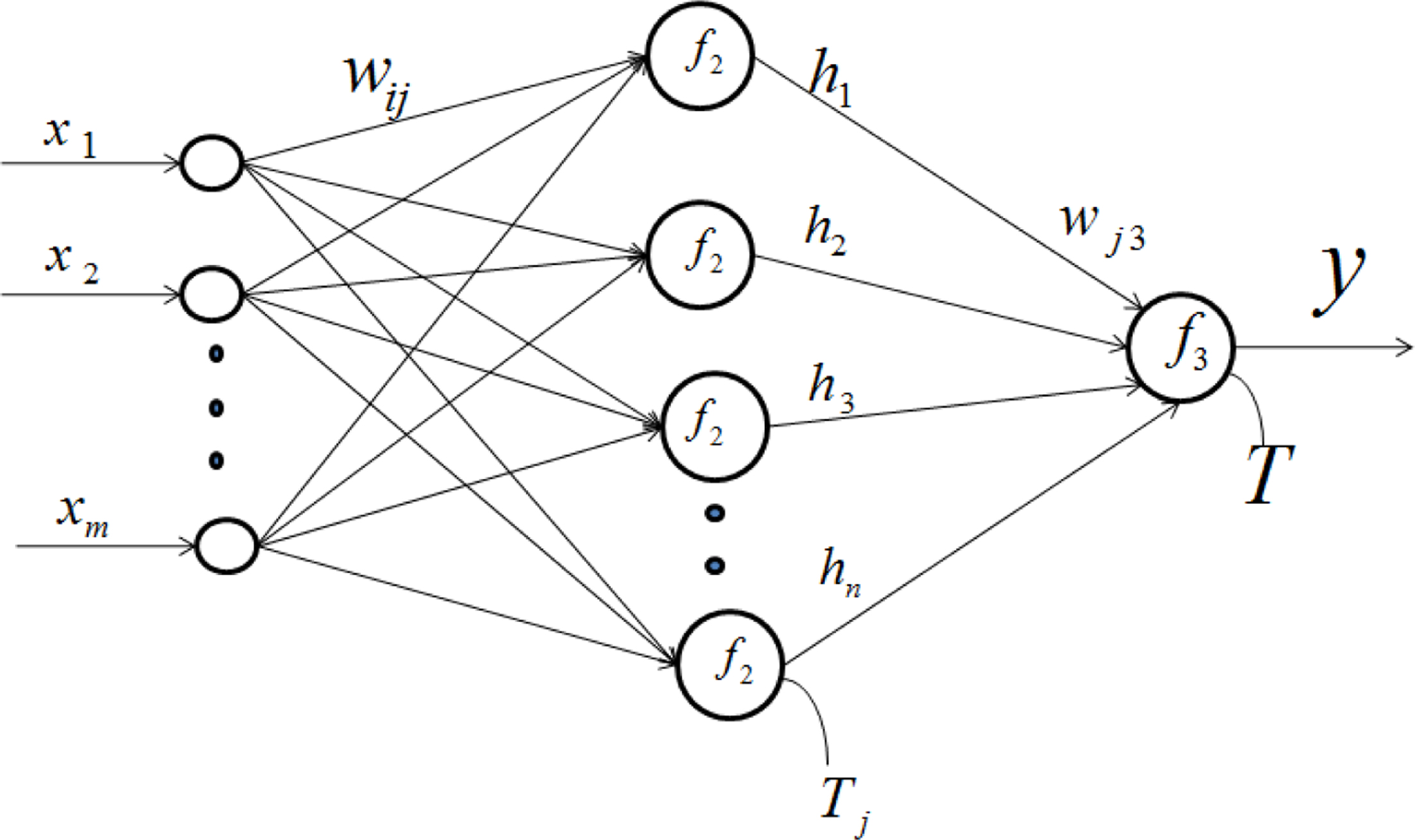

Out put of the MLP network ‘ $y$ ’ is calculated as

$\displaystyle y=f_{3}\left(\sum\limits_{j=1}^{N}{w}_{j3}h_{j}-T\right).$ (4)

where, $N$ is the number of neurons in the hidden layer, $w_{j3}$ is the weight between hidden layer to the output neuron, $h_{j}$ is the output of neuron $j, T$ is the threshold of the output neuron and $f_{3}$ is the sigmoid activation function of the output neuron. Output of the hidden layer is calculated as:

$\displaystyle h_{j}=f_{2}\left(\sum\limits_{i=1}^{M}{w}_{ij}x_{i}-T_{j}\right).$ (5)

where, $w_{ij}$ are the weights from the input neurons to neuron $j$ in the hidden layer, $x_{i}$ are the input data and $T_{j}$ is the threshold of neuron $j$ , and $f_{2}$ is the sigmoid activation function of the hidden neuron. The MLP neural networks may use different types of learning techniques for training purpose as discussed below

3.1.1 MLP with back-propagation learning

Back-propagation learning allows supervised lear-ning procedure where desired output is known by the network before training process. Learning occurs by changing connection weights based on the amount of error in the output. Error produced in the output propagate towards backward direction to the network for minimizing the error produced by the network. It uses gradient descent method for minimizing the error in weight space because weight is the solution of the learning problem. If the state of system moving in the opposite direction to the largest local scope then weight are updated in downward direction [40, 41, 42, 43, 44, 45, 46, 47]. An activation function is used in the hidden layer and output layer which compute the gradient of error as shown in Fig. 2.

Figure 2.

Back-propagation of errors for a single neuron.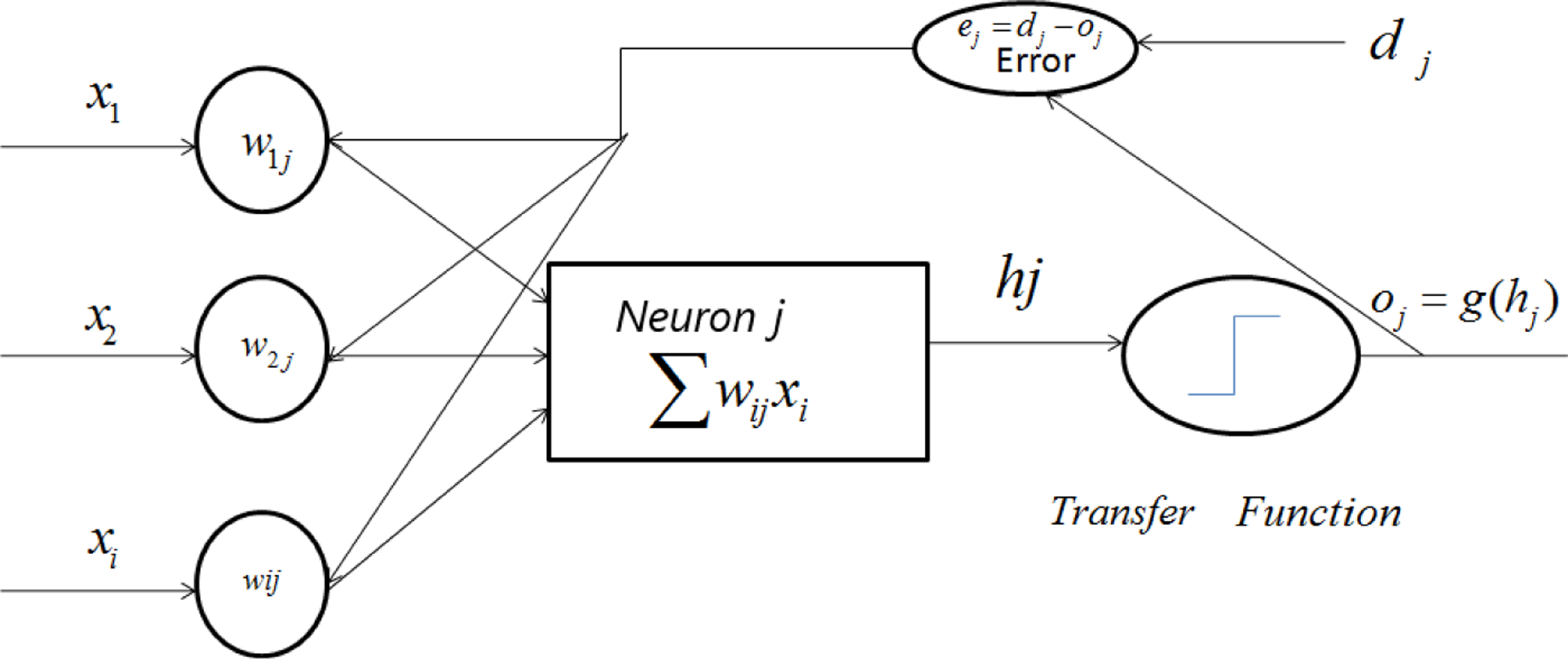

$E(n)$ is the error of whole network which is calculated as follows:

$\displaystyle E(n)=\sum_{j=1}^{p}e_{j}^{2}(n).$ (6)

where, $p$ is the size of the training set. MLP network can also be trained with Bayesian learning technique as discussed in the next subsection.

3.1.2 MLP with Bayesian learning

Bayesian network is a directed acyclic graph, used for regression, classification, and inverse problem [48, 49, 50, 51]. In Bayesian learning entire distribution of model prediction estimation is done instead of the mean prediction estimation of the model. This estimation take noise in the data and variance of the model. For all unknown data Bayesian approach produce posterior probability distributions [52, 53, 54, 55]. In Bayesian learning for MLP neural network the natural end variables are the predictions of the model for new input. For input $x_{k}$ and training data $D={(x_{1},y_{1}),(x_{2},y_{2}),\ldots(x_{k},y_{k})}$ , for the output $y_{k}$ posterior predictive distribution is calculated by integrating the predictions of the model with respect to the posterior distribution of the model,

$\displaystyle p(y_{k+1}|x_{k+1},D)$ $\displaystyle\quad=\int p(y_{k+1}|x_{k+1},\theta)p(\theta|D)d.$ (7)

where, $\theta$ denotes all the model parameters and hyper parameters of the prior structures [56, 57, 58].

The MLP neural network uses many layers and many hidden neurons in each layer, which potentially increases the complexity of the overall network. So, we can also use the simpler RBFN models to predict the exchange rate of any country having less complex neural networks, which is discussed in the next Section.

3.2 Exchange rate prediction using radial basis function network

RBFN is a simple neural network having powerful problem solving ability. Name of the network is RBFN because it uses radial basis activation function. It has three layers, that are input layer, hidden layer and output layer as shown in Fig. 3. In the input layer data are given to the network, then this input multiply with the weight and given to the hidden layer. $c_{k}$ is the cluster vector in this hidden layer and there must be cluster element $c_{ik}$ ( $i=1$ to $N,k=1$ to $L$ ) where $N$ and $L$ are number of input node and hidden node respectively [46, 47, 48, 49, 50, 51]. Each node in the hidden layer calculates the Euclidean distance between cluster head and the input and basically Gaussian type radial bias function is used as activation function [52, 53]. The out put of the hidden layer multiplies with weight are given to the output layer.

Figure 3.

Architecture of RBF neural network.

The distance between the input node and hidden node are calculates as:

$\displaystyle Dst_{k}=|x-c_{k}|=\sqrt{\left(\sum_{j=1}^{n}(x_{j}-{c_{k}})^{2}% \right)}.$ (8)

Radial basis activation function is used to transforms the Euclidean summation $Dst_{k}$ to give an output for each node. This function also has a basis width $\sigma_{k}$ and out put is $\phi_{k}$ , which is calculated as:

$\displaystyle\phi_{k}=\exp\left(\frac{-Dst_{k}^{2}}{\sigma_{k}^{2}}\right).$ (9)

The out put of the RBFN is calculated as:

$\displaystyle Y_{k}=\phi_{k}*W_{k}^{T}.$ (10)

The error is calculated as

$\displaystyle e_{n}=Y_{k}(n)-Y_{d}(n).$ (11)

where, $Y_{k}(n)$ is the model output and $y_{d}(n)$ is the desired output. Both supervised and unsupervised learning is used in RBFN. Unsupervised learning is used to decide weight value $w_{1}$ from input layer to hidden layer. Then supervised learning is used to train the weight value $w_{2}$ hidden layer to output layer. Number of hidden layer node start from 0 and increases automatically by means of checking the output errors. During each iteration it take input vector and weight value vector $w_{1}$ and form a new hidden layer and check the error of the net again. This process is repeated until we reach the acceptable error [59, 60, 61, 62, 63]. For better accuracy we can use combination of more then one RBFN networks, which is discussed in the next Section.

3.2.1 Multistage radial basis function network

Combination of RBFN models produce less amount of error and gives better result than single RBFN model. So a multistage RBFN model was develop where numbers of single RBFN are combine together and consider as a single RBFN model [64, 65, 66, 67, 68, 69, 70]. A multistage RBFN have three stage as shown in Fig. 4 and are presented as:

Figure 4.

Architecture of multistage RBF neural network.

a. a.

Producing multiple single RBFN predictorsPerformance of a RBFN depends on number of node in the hidden layer, cluster center, width of cluster and on the training data, so in the first stage multiple number of RBFN are produced by varying the number of node in the hidden layer or by changing the cluster center or by adopting different cluster radius of the RBFN neural networks or by using different training data.

Choosing appropriate ensemble membersEvery RBFN produced different result when input data are given to it, generally PCA (Principle Component Analysis) technique is used to choose appropriate RBFN having less amount of error in order to increase network efficiency. However, the PCA is a kind of data-reduction technique, which does not consider the internal correlations between different ensemble members. To overcome this problem, a Conditional Generalized Variance (CGV) minimization meth-od is proposed.

Combining the selected membersAfter selecting the appropriate model the out put of all the model are combine and final output is produced $y=f(x)$ ,

$f(x)=\displaystyle\sum\limits_{i=1}^{m}w_{i}f_{i}(x).{}$

where, $w_{i}$ is the weight of $f_{i}(x)$ . Four method are used for determining weight in the network. That are simple averaging, simple MSE, stacked regression method and variance – based weighting method.

We can also use another simple technique such as FLANN to predict the exchange rate, which is discussed in the next Section.

3.3 Functional link artificial neural network for exchange rate prediction

FLANN is a single layer artificial neural network. It is capable of performing complex decisions i.e. it can work with nonlinear data with out hidden layer [71, 72, 73, 74, 75, 76, 77]. Hidden layer is removed to reduce its computational cost. Inputs are functionally expanded using some trigonometry expansion. Let’s consider a two dimensional input $x=[x_{1}∼{}x_{2}]^{T}$ . The enhanced pattern is obtained by using trigonometric function $x^{*}=[X_{1}\cos(\pi x_{1})\sin(\pi x_{1})\ldots X_{2}\cos(\pi x_{2})\sin(\pi x% _{2})\ldots$ $X_{1}X_{2}]$ which, is used by network for equalization purpose. Block diagram of FLANN is given in Fig. 5. FLANN consists of 3 process.

a. a.
Functional expansion process: In this input element is nonlinearly expanded to create numbers of inputs. The number of element after expansion becomes more than original input.
b.
Estimation process: It compute the output of adaptive model and generate the error signal.
c.
Adaptive process: It adjust the weight by weight update learning rule.

The learning process of FLANN is given in the next Section.

Figure 5.
Block diagram of FLANN.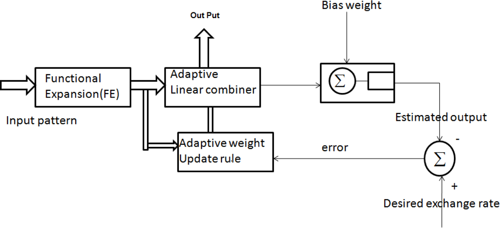

3.3.1 FLANN with back-propagation learning

FLANN use back-propagation learning algorithm for training the network [78, 79, 80, 81, 82]. Error produced by it is calculated by substituting the estimated output from desired output and propagate backward for weight updating using weight update rule as shown in Fig. 6.

Figure 6.

Architecture of FLANN.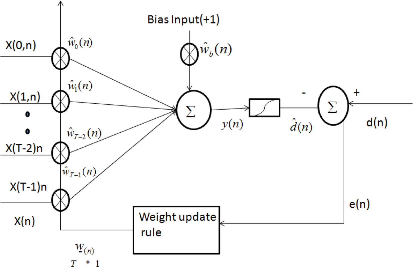

Let $q$ is the total number of input, $M$ is the number of patterns used for training the network, $N$ is the number of pattern used for testing. Input element consist of $P$ feature element and $m$ , $p$ are input pattern and feature number respectively for a matrix $d(m,p)$ such that $0\leqslant m\leqslant M-1,0\leqslant p\leqslant P-1$ . If $\rm U$ is the input feature matrix having dimension $(M*P)$ . Each row of $U$ is denoted as $D_{n}$ which is functionally expanded using sine and cosine function as $s(m,p(2k+1))=D(n,0)$ , $s{m,(2k-1)}=\sin[{(2k-1)\pi}.d(n,m)]$ . $s(m,2k)=cos[(2k-1)\pi.d(n,m)],{k=1,2}\ldots,{k}$ and ${p=0,1}\ldots{(P-1)}$ . Where, $K$ is the number of sine and cosine expansion. After expansion $S$ matrix is generated. Each row of $S$ is denoted as ${X(m)}$ which is of size $(T*1)$ . Where, $T=P(2k+1)$ and $X(m)=[s(m,0),s(m,1)s(m,2)\ldots s(m,t)]^{T}$ . In training process each input pattern $x(m)$ applies sequentially, then multiply with weight vector and passes through activation function and output of model is produced as follows:

$\displaystyle Y(m)=X^{T}(m).\hat{W}(m)+\hat{w}_{b}(m).$ (12) $\displaystyle\hat{d}_{1}(m)={f(X,m)}=\frac{1-e^{-y(m)}}{1+e^{-y(m)}}.$ (13)

where, the system output is denoted as $\hat{d}_{1}(m)$ , and $d_{1}(m)$ is the desired output. Error is calculated as the difference between the desired output and system output $e(m)=d_{1}(m)-\hat{d}_{1}(m)$ . Then error and input vector are applied to weight updated algorithm to compute correction weight vector as follows:

$\displaystyle\delta(m)=e(m)\hat{d}^{\prime}(m)=e(m)f^{\prime}{y(m)}.$ (14)

Then the correction weight vector is given by

$\displaystyle\Delta\hat{w}(m)=\eta x(m).\delta(m).$ (15)

The change in bias weight can be obtained and is given by

$\displaystyle\Delta\hat{w}_{b}(m)=n\delta(m).$ (16)

where, $\eta$ is the learning coefficient which lies between 0 and 1. Average change of weight of $t_{th}$ weight in $i_{th}$ experiment is given by

$\displaystyle\Delta\hat{w}a_{t}(i)=\frac{1}{M}\sum\limits_{m=1}^{M}\Delta\hat{% W}_{t}(m).$ (17)

Weight are updated as follows

$\displaystyle\hat{w}(i+1)=\hat{w}(i)+\Delta wa(i).$ (18)

Change of bias is calculated as follows

$\displaystyle\Delta\hat{w}a_{b}=\frac{1}{M}\sum\limits_{m=1}^{M}\Delta\hat{w}_% {b}(m).$ (19)

Bias will be updated as

$\displaystyle\hat{w}_{b}(i+1)=\hat{w}_{b}(i)+\Delta\hat{w}a_{b}.$ (20)

Experiment is continue until MSE will reach a minimum value. MSE will be calculated as

$\displaystyle\textit{MSE(i)}=\frac{1}{M}\sum\limits_{m=1}^{M}e^{2}(m).$ (21)

When, the training process is completed weight are fixed with the new value and the testing process will be conducted. We can also use CFLANN to predict the exchange rate as discussed in the next subsection.

3.3.2 Cascaded FLANN

In this model two single FLANN are connected in series as shown in Fig. 7. Each FlANN are passed through back-propagation algorithm and output of first FLANN given to the second FLANN as its input. This value also expanded using trigonometric function [83, 84, 85, 86, 87]. The block diagram of CFLANN is presented in Fig. 7.

Figure 7.

Block diagram of CFLANN.

Where, FL1 is the first FLANN and $\hat{d}_{1}(m)$ is the output of first FLANN, which is calculated as follows:

$\displaystyle\hat{d}_{1}(m)=\frac{1-e^{-y(m)}}{1+e^{-y(m)}}.$ (22)

and the output $Y(m)$ is calculated as in FLANN.

$\hat{d}_{1}(m)$ is expanded by trigonometric expansion as follows:

$\displaystyle s_{2}(m,0)=\hat{d}_{1}(m).$ (23) $\displaystyle s_{2}(m,2l-1)=\sin[{(2l-1)\pi}.\hat{d}_{1}(m)].$ (24) $\displaystyle s_{2}(m,2l)=\cos[{(2l-1)\pi}.\hat{d}_{1}(m)].$ (25)

The operational principle is same as single FLANN till we get a minimum MSE. In the next Section we have analysed some of the statistical models integrated with neural networks.

4. Auto-regressive integrated moving average model

ARIMA models are generally combination of autoregressive (AR) and moving average model (MA), a non seasonal ARIMA model is denotes ARIMA $(p,d,$ $q)$ where parameters $p, d,$ and $q$ are non-negative integers is the order of the Autoregressive model, $d$ is the degree of differentiae, and $q$ is the order of the moving-average and a seasonal ARIMA model is denoted as ARIMA $(p,d,q)_{m}$ where m is the number of period. Autoregressive mode having order $p$ is represented as

$\displaystyle Z_{t}=\phi_{1}Z_{t-1}+\phi_{2}Z_{t-2}\ldots+\phi_{k}Z_{t-p}.$ (26)

AR represent the current time series value $Z_{t}$ from the previous time series value. $Z_{t-1},Z_{t-2}\ldots Z_{t-p}$ , and $\phi_{1},\phi_{2}\ldots.\phi_{z}$ are auto regressive coefficient. Moving average model having order r is represented as

$\displaystyle Z_{t}=E_{t}-\theta_{1}E_{t-1}-\theta_{2}E_{t-2}\ldots,-\theta_{r% }E_{t-r}.$ (27)

$E_{t-1},E_{t-2}\ldots,E_{t-r}$ are independent white noise sequence having mean value $\bar{x}$ and variance $\sigma^{2}$ and $\theta_{1},\theta_{2}\ldots\theta_{r}$ are moving average coefficient. By integrating AR and MA model final model ARIMA model is found and it is represented as

$\displaystyle(1-B)^{d}Z_{t}=[{{\theta(B)}/{\phi(B)}}]E_{t}.$ (28)

where, $t$ is the time factor and $B$ is called the back shift operator and represented as

$\displaystyle BZ_{t}=Z_{t-1}.$ (29)

where, $\phi(B)$ and $\theta(B)$ are autoregressive and moving average coefficient respectively and represented as

$\displaystyle\phi(B)=1-\phi_{1}B^{1}-\phi_{2}B^{2}\ldots\phi_{k}B^{k}.$ (30) $\displaystyle\theta(B)=1-\theta_{1}B^{1}-\theta_{2}B^{2}\ldots\theta_{r}B^{r}.$ (31)

We can also use integrated ARIMA model with neural networks to produce better results as discussed in the next Section.

5. An integrated model using ARIMA, MLP AND RBF

An integrated model is produce by using ARIMA, MLP and RBF model. In this model real exchange rate is called relax and predicted exchange rate is called arimaout. First the time series data is given to the ARIMA model and the produced output and error is called error1 as shown in Fig. 8.

Figure 8.

Error in ARIMA model.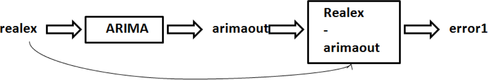

Error1 is the error produced by ARIMA model. This error1 is given to MLP and result is mlperror as shown in Fig. 9.

Figure 9.

Error in MLP model.

Relax $=$ arimout $+$ mlperror RBFN is used to further reduced the error. Output of ARIMA is added to output of MLP and the remainder of this result and the real exchange rate will be called error2 and given to the RBFN as shown in Fig. 10.

$\displaystyle{\rm Error2}={\rm realex}-{\rm(arimaout+mlperror)}$

The final result of the proposed integrated model comes from the summation of the error modeled by RBFN and the error modeled by MLP with the time series that was modeled by ARIMA [88, 89, 90, 91, 92, 93, 94]. Final model is given in Fig. 11.

Figure 10.

Error in RBFN model.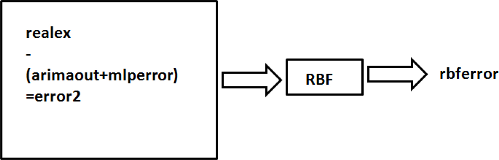

Figure 11.

Integrated model using MLP, RBFN and ARIMA.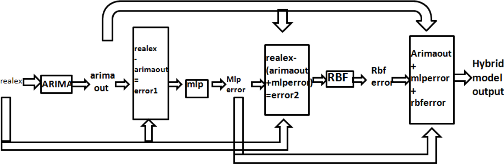

6. Empirical study

In this review paper different models are analysed that takes different exchange rates from different countries with varying time duration. The number of training and testing data are also vary with different types model and are described in this Section.

6.1 Dataset preparation

In this Section we have explained the various type of data used in different models for their analysis. Each set of data are normalized by dividing each value by the maximum value of each set such that each normalized value is less than or equal to unity.

a. a.
MLP with back-propagation learning For this model data has been collected as follows

1. 1.
Daily datasetDaily exchange rate of EUR/USD, GBP/USD, USD/JPY are taken from the site. http://www.global-view.com/forex-trading-tools/forex-history/index.html. Data are collected for the period from 1 Jan 2014 to 25 Apr 2014. From 78 training vectors 60 vectors are used for the training and 18 for the testing.
2.
Monthly datasetThe monthly exchange rate of EUR/USD, GBP/ USD, USD/JPY are taken from. http://www.oanda.com/currency/historical-rates/. Da-ta are c-ollected for the period from May 2009 to May 2014. From 55 training vectors 40 vectors are used for the training and15 for the testing.
3.
Quarterly datasetThe quarterly data of EUR/USD, GBP/USD, USD/JPY are taken from site: http://www.oanda.com/currency/historical-rates. Data are collected for the period from May 1999 to May 2014. From 54 training vectors 42 vectors are used for the training and 12 for the testing.

b.
MLP with BAYESIAN LearningFor this model data has been collected as: U.S. dollar against the British Pound (GBP/USD) and Japanese Yen (JPY/USD) from Jan 1990 to Dec, 2002 are taken daily wise, which was given by Professor Werner Antweiler, University of British Columbia, Canada. Sixty patterns are used for testing and rest of the data are taken for training the network.
c.
RBF CNY Exchange Rate For this model data has been collected as follows GBP – CNY and USD – CNY, are taken from 27-Apr-2005 to 12-Feb-2009, and from 1-Apr-2005 to 13-Feb-2009 respectively. The daily closing price of the two spot exchange rates were found on the Web site: http://www.bankofengland.co.uk/statistics/,which is the official Web site of Bank of England. In GBP – CYN from 956 input data first 900 data were used for training, and the remaining 56 data were used for testing. In USD – CYN total number of input samples to the network is 976, from which first 900 data were used for training, and the remaining 76 data were used for testing.
d.
Integrated modelFor this model data has been collected as follows EUR/USD (Euro to US Dollar) exchange rate is used for the model design, validation and testing. The data are taken from the Federal Reserve Bank of St. Luis, economics research center’s web site. The data set from 1 April 2001 to 31 July 2010 are taken and 7:2:1 ratio is used for training, validation and testing purpose.
e.
Multistage RBFData are obtained from site: http://fx.sauder.ubc.ca/, provided by Professor Werner Antweiler, University of British Columbia, Vancouver, Can-ada. US dollar against each of the four currencies British pounds (GBP), euros (EUR), German marks (DEM) and Japanese yen (JPY), from January 1971 to December 2000 used for training and data from January 2001 to November 2006 used for testing.
f.
FLANN and CFLANNFor this model data has been collected as follows: Exchange rate of US dollar to Pound, Rupees and Yen are taken. Some common features from past conversion rates are extracted for training and testing purposes. Each set of data are normalized by dividing each value by the maximum value of each set such that each normalized value is less than or equal to unity. Normalization of input data is necessary for obtaining correct trigonometric expansion.

6.2 Environment and parameters setting

In this work, most of the models have used neural network tool box provided by Matlab software package. The author has taken one input variable, six hidden nodes and 6000 iterations to compare NN models with RW, GARCH, and ARIMA model. For MLP neural networks the authors have used (7-6-5-1), (7-4-2-1) and (5-10-1) network architectures and for RBF neural networks the authors have used (7-11-1) and (7-9-1) network structures. The learning parameters for learning algorithm of MLP neural network were eta $=$ 0.3 and alpha $=$ 0.9, and for the RBF neural network, the learning parameters were eta $=$ 0.4 and alpha $=$ 0.9. In ARIMA model ARIMA (1, 1, 4) architecture was used. Each set of data are normalized by dividing each value by the maximum value of each set such that each normalized value is less than or equal to unity.

6.3 Error function

In this Section, we have discussed various error functions as follows:

We can determine the error of a system as Root – mean – square error and can be calculated as follows

$\displaystyle\textit{RMSE}=\sqrt{\sum_{t=1}^{T}(\hat{Y_{i}}-Y_{i})^{2}}.$ (32)

where, $Y$ is the original time series value and $\hat{Y}$ is the predicted value. $T$ is the number of values in the time series, or in the test set of the time series. The RMSE shows the error in terms of the level and not the direction. Mean absolute error (MAE) is a measure of difference between two continuous variables. Assume $X$ and $Y$ are variables of paired observations that express the same phenomenon. MAE is the average vertical distance between each point and the $Y=X$ line, which is also known as the One-to-One line. Mathematically MAE can be presented as:

$\displaystyle\textit{MAE}=\frac{\sum_{i=1}^{n}\left|\hat{Y_{i}}-Y_{i}\right|}{n}$ (33)

where, $\hat{Y}$ is a vector of $n$ predictions, and $Y$ is the vector of observed values corresponding to the inputs to the function which generated the predictions. MAPE is a measure of prediction accuracy of a forecasting method in statistics. It usually expresses accuracy as a percentage, and is defined by the formula:

$\displaystyle\textit{MAPE}=\frac{100}{n}\left(\sum_{i=1}^{n}\left|\frac{\hat{Y% _{i}}-Y_{i}}{Y_{i}}\right|\right)$ (34)

where, $\hat{Y}$ is a vector of $n$ predictions, and $Y$ is the vector of observed values corresponding to the inputs to the function which generated the predictions. The ability to predict movement direction or turning points can be measured by a statistic. The NMSE (Normalised Mean Square Error) is an estimator of the overall deviations between predicted and measured values. It is defined as:

$\displaystyle\textit{NMSE}=\frac{1}{N}\sum_{i}^{n}\frac{\left(\hat{Y}-Y\right)% ^{2}}{\bar{\hat{Y}}\bar{Y}}$ (35) $\displaystyle\bar{Y}=\frac{1}{N}\sum Y_{i}$ (36) $\displaystyle\bar{\hat{Y}}=\frac{1}{N}\sum\hat{Y_{i}}$ (37)

where, $\hat{Y}$ is a vector of $n$ predictions, and $Y$ is the vector of observed values corresponding to the inputs to the function which generated the predictions. The ability to predict movement direction or turning points can be measured by a Directional change statistics ( $D_{\textit{sat}}$ ) can be expressed as $D_{\textit{sat}}$ .

$\displaystyle D_{\textit{sat}}=\frac{1}{T}\sum_{t=1}^{T}a_{t}.$ (38)

if $(x_{t+1}-x_{t})(\hat{x}_{t+1}-x_{t})\geqslant 0$ then $a_{t}=1$ , else $a_{t}=0$ and $T$ is the number of testing samples.

Table 1

Error in The MLP with back – propagation learning

Exchange rate	Daily error	Monthly error	Quarterly error
	Avg – max	Avg – max	Avg – max
EUR/USD	0.2–0.4	1.3–3.3	2.3–5.1
GBP/USD	0.2–0.9	2.2–4.5	1.9–5.0
USD/JPY	0.3–1.3	0.3–1.3	3.5–10.2

Table 2

Error in neural network models (GBP/USD)

Input nodes	BPNN	Bayesian learning MLP
3	0.005471	0.005468
5	0.004491	0.004482
7	0.004496	0.004494
9	0.005467	0.005465

Table 3

Error in the neural network models (JPY/USD)

Input nodes	BPNN	Bayesian learning MLP
3	0.007438	0.007121
5	0.006348	0.006302
7	0.006358	0.006285
9	0.007293	0.006994

Table 4

Error produced in different models

EUR/USD	Integrated	Single	Single	Single
	model	ARIMA	MLP	RBF
RMSE	0.0068	0.0081	0.0076	0.0085
$D_{\textit{sat}}$ (%)	71	65	67	59

6.4 Results and analysis

In this Section we have analysed the performance of different models and we have determine which model produces less amount of error and more accurate output based on the survey analysis. The details of the analysis are given below. At last we have provided a comparison table for the above analysis.

6.4.1 MLP with back-propagation learning

Table 1 shows the daily, monthly and quarterly error rate of different exchange rates using MLP with back propagation learning. The prediction results with daily, monthly and quarterly step are depicted in Figs 12–20 for EUR/USD, GBP/USD and USD/JPY. These results show that the short-term prediction method using MLP provides good accuracy of the prediction.

Figure 12.

Prediction of exchange rate EUR/USD with daily step.

Figure 13.

Prediction of exchange rate GPB/USD with daily step.

Figure 14.

Prediction of exchange rate JPY/USD with daily step.

Figure 15.

Prediction of exchange rate EUR/USD with monthly step.

Figure 16.

Prediction of exchange rate GPB/USD with monthly step.

Figure 17.

Prediction of exchange rate JPY/USD with monthly step.

Figure 18.

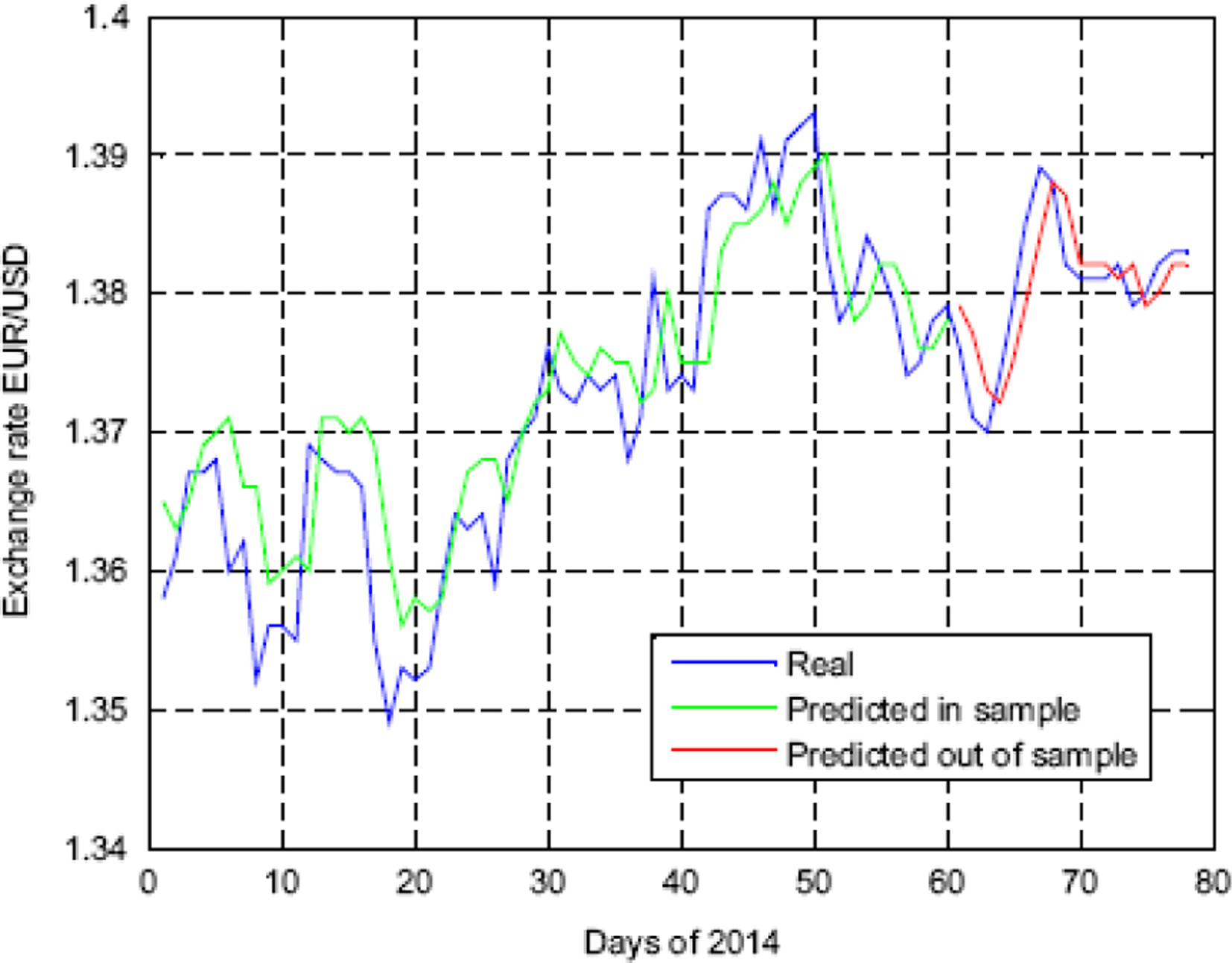
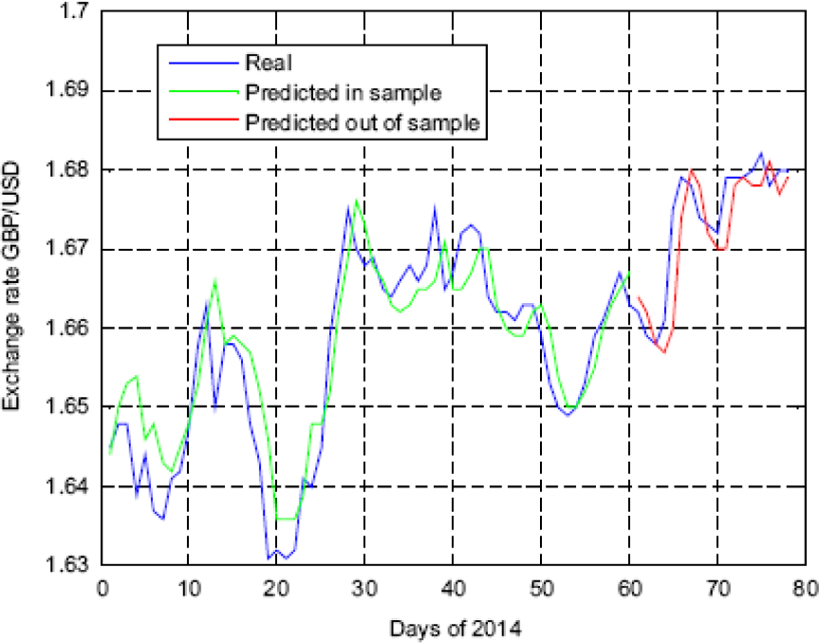
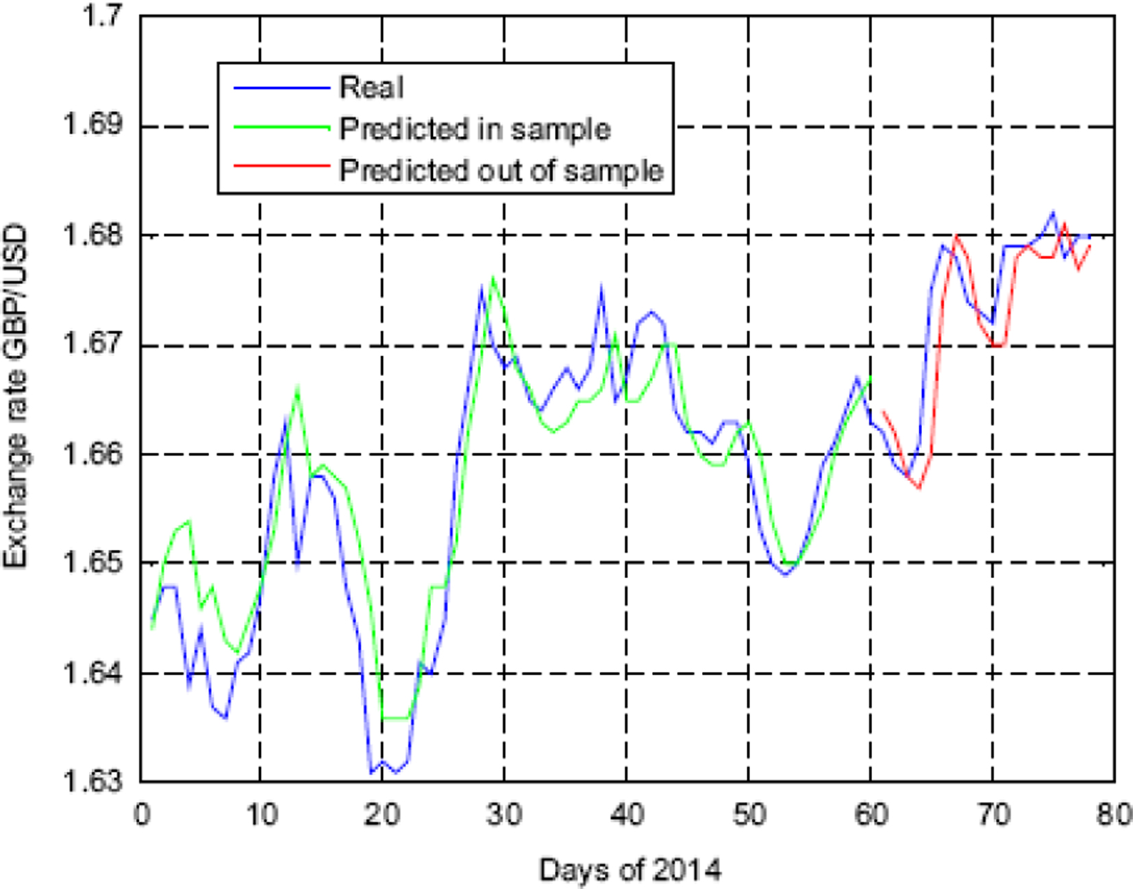
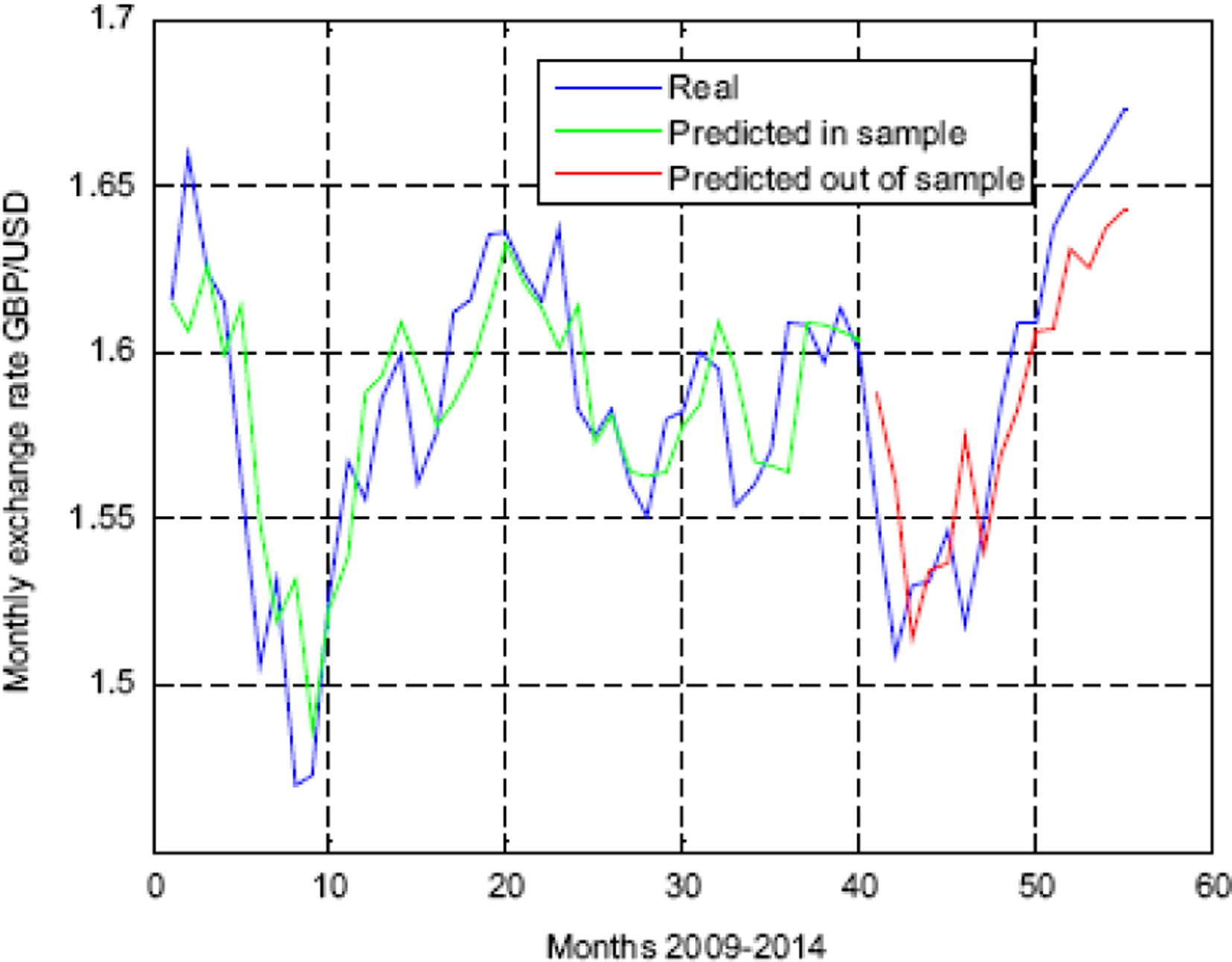
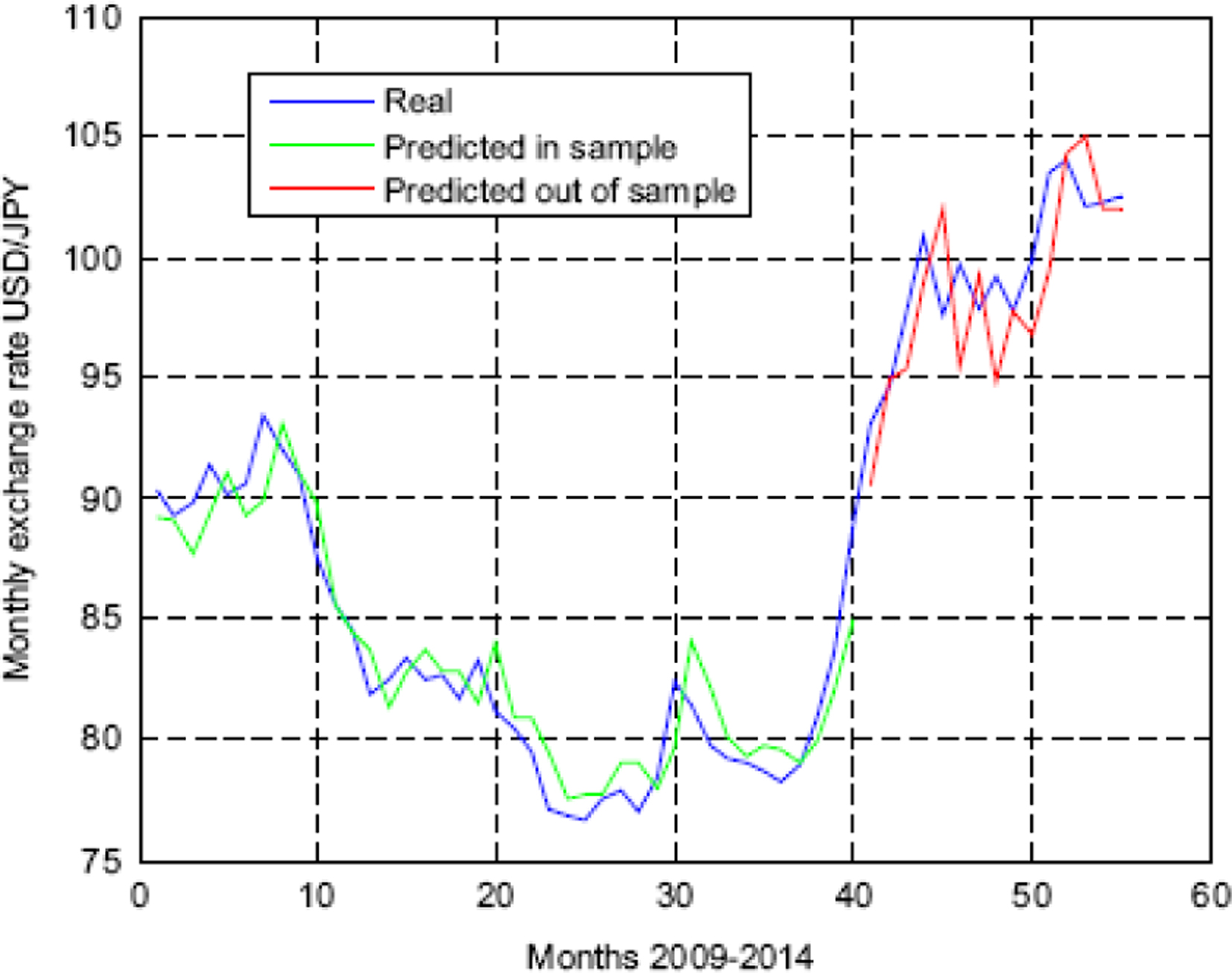
Prediction of exchange rate EUR/USD with quarterly step.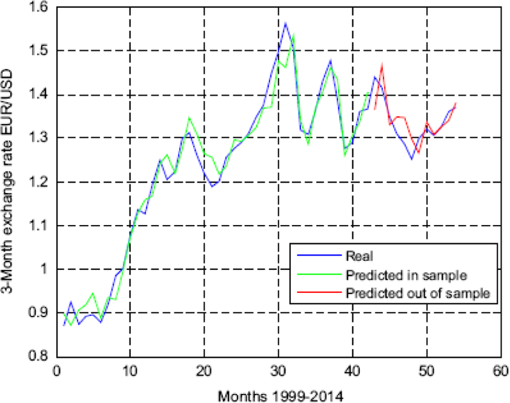

Figure 19.

Prediction of exchange rate GBP/USD with quarterly step.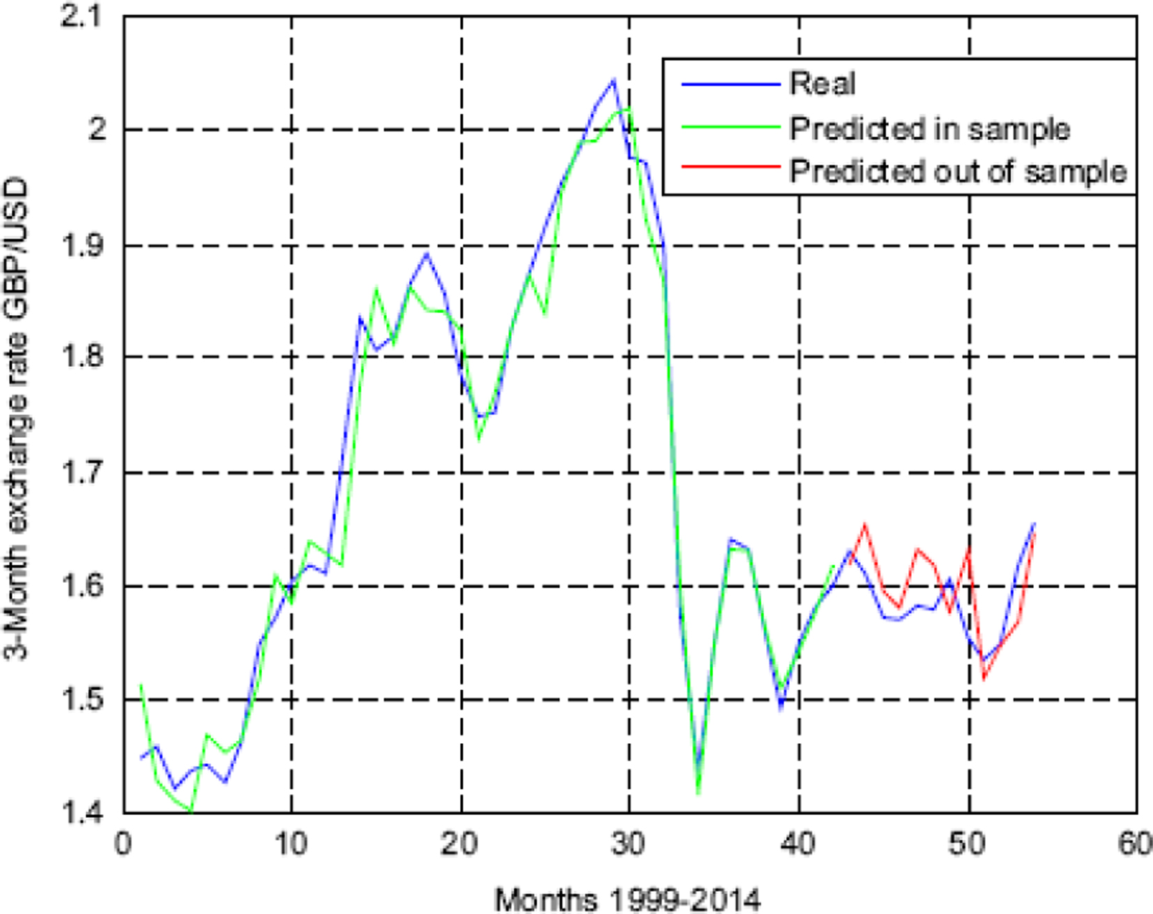

Figure 20.

Prediction of exchange rate JPY/USD with quarterly step.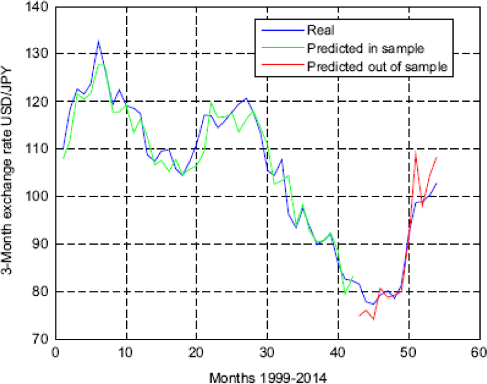

6.4.2 MLP with Bayesian learning

Tables 2 and 3 show the error rate of GBP/ USD and JPY/USD exchange rates using MLP with Bayesian learning. The experimental results shows that predicting exchange rates using MLP with Bayesian learning is producing better results than BPNN model.

6.4.3 Performance of integrated model

In this Section we have compared the proposed integrated model to simple ARIMA and simple MLP and RBF in terms of error level with RMSE. Table 4 show the error rate of different exchange rates using Integrated model. The results from the Table 4 show that the integrated model works better than the other single models both in terms of error level and directional status.

6.4.4 Performance of multistage RBFN model

In this Section, four main currency exchange rates are used to test the proposed RBF neural network ensemble forecasting model. Tables 5 and 6 show the error rate of different exchange rates using Multi stage RBFN model. The low NMSE does not necessarily mean that there is a high hit ratio for foreign exchange movement direction prediction. Thus, the Dstat comparison is necessary for business practitioners. Focusing on Dstat of Table 6, it is not hard to find that the proposed RBF neural network ensemble forecasting model outperforms the other ensemble models and the single RBF model.

Table 5
NMSE of multistage RBF with different mode

Models	GBP	EUR	DEM	JPY
	NMSE – rank	NMSE – rank	NMSE – rank	NMSE – rank
Single RBF mode	0.0614-4	0.0862-5	0.8595-6	0.0942-5
Simple averaging	0.0686-5	0.0956-6	0.0812-5	0.0978-6
Simple MSE	0.0789-6	0.0724-4	0.0733-4	0.0825-4
Stack regression	0.0484-3	0.0668-3	0.0598-2	0.0767-3
Variance based model	0.0467-2	0.0545-2	0.0654-3	0.0596-2
Multistage RBF	0.0388-1	0.0451-1	0.0462-1	0.0511-1

Table 6

$D_{\textit{sat}}$ of multistage RBF with different model.

Models	GBP	EUR	DEM	JPY
	NMSE – rank	NMSE – rank	NMSE – rank	NMSE – rank
Single RBF mode	71.83-5	66.19-6	66.19-6	63.38-6
Simple averaging	67.61-6	71.83-4	76.05-4	70.42-5
Simple MSE	73.23-4	70.43-5	69.01-5	71.83-4
Stack regression	77.46-3	76.05-3	78.87-3	73.23-3
Variance based model	80.23-2	83.09-2	81.69-2	78.87-2
Multistage RBF	88.73-1	90.14-1	91.54-1	85.91-1

6.4.5 Performance of FLANN model

In this Section the authors have proposed two efficient low complexity neural network based forecasting models for exchange rate prediction. The first model is very simple with one layer and single neuron but with nonlinearly mapped input features. The second model consists of two stage FLANNs. The output of the first stage undergoes nonlinear expansion and then fed to the second FLANN for predicting the exchange rate. Computer simulation study of both the models reveal that each of them offer better prediction performance compared to the LMS model. However, out of the FLANN and CFLANN models, the later offers superior prediction performance in all cases. Table 7 shows the error rate of different exchange rates using FLANN and CFLANN model.

Table 7
Accuracy in FLANN and CFLANN

Month	Actual	LMS	FLANN	CFLAN
ahead
Rupees
conversion
1	45.63	44.20	44.6892	45.9620
3	44.20	44.78	44.7953	44.0019
6	44.82	44.78	44.9954	44.2958
12	45.97	42.83	45.2923	46.1454
Pound
conversion
1	0.5764	0.5524	0.5725	0.5776
3	0.5654	0.5181	0.5763	0.5651
6	0.5656	0.4926	0.5802	0.5698
12	0.5181	0.4716	0.5900	0.5283
Yen
conversion
1	118.45	114.78	115.3831	116.6212
3	115.48	113.68	115.4728	115.7532
6	117.07	111.89	116.4297	116.7695
12	111.00	108.00	121.6428	113.2557

6.4.6 Performance of neural network with random walk (RW), GRACH, and ARIMA models

Here, we have investigated whether NN models can offer improvements in terms of forecasting accuracy over RW models and extensively used ARIMA and GARCH models. Given that most rate data contain nonlinear structures, one would expect NN models to be able to exploit the nonlinear structures to provide better forecasts as NN models can approximate any continuous function to a good degree of accuracy without the imposition of the assumptions regarding the form of nonlinearity. The experimental analysys, indicate that NN models can provide better forecasts than RW models and traditional models, such as, ARIMA and GARCH models. The better performance of NN models is likely to have stemmed from the fact that they are nonlinear models, that can exploit the nonlinearity in the exchange rate data without the imposition of assumptions about the form of nonlinearity. Tables 8 and 9 show the daily exchange rate predictions of Australian dollar and British pound using linear and non-linear models. It has been observed from the experimental analysis that neural network (NN) models have lessor error rates than the other linear models.

Table 8
Out-of-sample forecasts of Australian dollar

Models	RMSE (RMSE/	MAE (MAE/	MAPE (MAPE/
	RMSE (RW))	MAE (RW))	MAPE (RW))
RW	0.006882 (1.000)	0.005185 (1.000)	2.865% (1.000)
ARMA	0.006981 (1.014)	0.005256 (1.014)	2.904% (1.012)
GARCH	0.006939 (1.008)	0.005237 (1.010)	2.893% (1.008)
NN	0.006835 (0.993)	0.005149 (0.993)	2.846% (0.992)

Table 9

Out-of-sample forecasts of British pound

Models	RMSE (RMSE/	MAE (MAE/	MAPE (MAPE/
	RMSE (RW))	MAE (RW))	MAPE (RW))
RW	0.003521 (1.000)	0.002743 (1.000)	0.3962% (1.000)
ARMA	0.003527 (1.002)	0.002754 (1.004)	0.3977% (1.004)
GARCH	0.003525 (1.001)	0.002746 (1.001)	0.3966% (1.001)
NN	0.003506 (0.996)	0.002733 (0.996)	0.3947% (0.996)

Table 10

Result analysis table

Technique used for prediction	Objective	Data used for training and testing	Result analysis
Neural Network, RW, GARCH and ARIMA.	Determine which data gives better result daily wise using NN, GARCH and ARIMA models.	GBP/USD, AUS/USD data are considered.	It has been observed that daily wise data gives less error in NN model in comparison to GW, GARCH and ARIMA models.
MLP with back propagation learning.	Determine which data gives better result daily wise, monthly wise or quarterly wise using back-propagation algorithm.	EUR, GBP/USD, USD/JPY data are considered.	It has been observed that daily wise data gives less error in comparison to monthly and quarterly wise.
MLP with Bayesian learning.	Train the network using Bayesian learning with varying the nodes.	GBP/USD, JPY/USD data are considered.	It has been observed that RMSE of BPNN is larger than Bayesian learning so Bayesian learning is performing better than BPNN.
Single MLP, Single RBF, Single ARIMA, Hybrid model (combination of MLP, RBF, ARIMA).	Train the network using different approaches and determining which model give minimum error.	EUR/USD data are taken from 1 April 2001 to 31 july2010.	Hybrid models are generating minimum amount of error.
Multistage RBF, Simple RBF, Simple averaging, Simple MSE, Stack regression, Variance based method used.	Determine performance of multistage RBF.	GBP, EUR, DEM, JPY data are taken from jan 1971 to dec 2000.	Multistage RBF produced less RMSE than other model.
FLANN and CFLANN.	Get best result using low complexity model.	Rupees, Yen, Pound are taken from jan 1971 to oct 2005.	CFLANN gives more accurate result than FLANN model.

6.5 Result analysis table

Finally in Table 10 we have summarised the whole experimental study on exchange rate prediction based on different types of statistical and biologically inspired algorithms.

7. Conclusions and future work

From the above empirical study we have analyzed that in MLP if daily exchange rate data are taken to train the network then error rate will be less in comparison to exchange rate data taken monthly and quarterly basis to train the network. MLP with Bayesian learning give better result than MLP with back propagation learning. Combination of RBFN gives more accurate result than single RBFN network. The performance of integrated model with combination of RBFN, MLP, ARIMA is better than individual model. To avoid complexity and for better result FLANN can be used to predict the exchange rates of different countries. Combination of FLANN which is called CFLANN gives more accurate result than individual FLANN. From this intensive empirical study we have concluded that no single model in this study consistently outperforms the others. The forecast capability of a particular model depends on the exchange rate of interest and the forecast horizon. Given the uncertainty in selecting a model, the combined forecasts seem to have an edge over the others and in general have relatively smaller RMSE ratios and higher percentage in predicting the direction of changes correctly. In spite of the attractiveness of combining forecasts, it should be stressed that forecasting exchange rate movement is still a daunting task. The forecasts of exchange rates from any of these models should be used with caution. For the forecast-performance comparison of the models, the results suggest that in future we can involve exchange rates of different developed, under developed countries and better optimised biologically inspired algorithms to increase the prediction accuracy. We can perform fine tuning of the parameters by using biologically inspired optimization algorithms to get better performance. This will open a broad research domain for the researchers. Time series forecasting is a fast growing area of research and as such provides many scope for future works. One of them is the Combining Approach, i.e. to combine a number of different and dissimilar methods to improve forecast accuracy. A lot of works have been done towards this direction and various combining methods have been proposed in literature. Together with other analysis in time series forecasting, we have thought to find an efficient combining model, in future if possible. With the aim of further studies in time series modeling and forecasting, here we conclude the present paper.

Footnotes

Conflict of interest

We do not have any conflict of interest with other authors.

References

Kathryn

. Are foreign exchange forecasts rational? New Evidence from Survey Data. Economics Letters. 1986; 21: 277-82.

Charles

. The forward discount anomaly and the risk premium: A survey of recent evidence. Journal of Empirical Finance. 1996; 3(2): 123-192.

Ronald

. Expectations formation and risk in three financial markets: Surveying what the surveys say. Journal of Economic Surveys. 2000; 14(1): 69-100.

Amiri

. An integrated eigenvector-DEA-TOPSIS methodology for portfolio risk evaluation in the FOREX spot market. Expert Syst. Appl. 2010; 37: 509-516.

Wang

Huang

Wang

. A novel text mining approach to financial time series forecasting. Neurocomputing. 2012; 83: 136-145.

Gill

Goel

. Indian currency exchange rate forecasting using neural networks. IEEE Conference Publications. 2010; 3: 196-199.

Galeshchuk

. Neural networks performance in exchange rate prediction. Neurocomputing. 2016; 172: 446-452.

Chiang

. Complex neurofuzzy ARIMA forecasting “a new approach using complex fuzzy sets”. IEEE Transactions on Fuzzy Systems. 2013; 21(3): 567-584.

TrucÄ±os

Luiz

, Hotta. Bootstrap prediction in univariate volatility models with leverage effect. Mathematics and Computers in Simulation. 2016; 120: 91-103.

10.

Thombs

Schucany

. Bootstrap prediction intervals for autoregression. J. Amer. Statist. Assoc. 1990; 85: 486-492.

11.

Calheiros

Masoumi

Ranjan

Buyya

. Workload prediction using ARIMA model and its impact on cloud applications QoS. IEEE Transactions on Cloud Computing. 2015; 3(4): 449-458.

12.

Wongsathan

Seedadan

. A hybrid {ARIMA} and neural networks model for PM-10 pollution estimation: The case of chiang mai city moat area. International Electrical Engineering Congress, iEECON2016, 2-4 March 2016, Chiang Mai, Thailand. 2016; 86: 273-276.

13.

Hoori

Motai

. Multicolumn RBF network. IEEE Transactions on Neural Networks and Learning Systems. 2017; 99: 1-13.

14.

Kia

Fathian

Gholamian

. Using MLP and RBF neural networks to improve the prediction of exchange rate time series with ARIMA. International Journal of Information and Electronics Engineering. 2012; 2: 543-546.

15.

Rout

Setty

. Efficient forecasting of exchange rates with recurrent FLANN. IOSR-JCE. 2013; 13: 21-28.

16.

Majhi

Rout

Majhi

Panda

Fleming

. New robust forecasting models for exchange rates prediction. Expert Systems with Applications. 2012; 39: 12658-12670.

17.

Naik

Nayak

Behera

. A global-best harmony search based gradient descent Learning {FLANN} (GbHS-GDL-FLANN) for data classification. Egyptian Informatics Journal. 2016; 17(1): 57-87.

18.

Cheng

Chen

Jenfu

. Financial distress prediction by a radial basis function network with logit analysis learning. Computers and Mathematics with Applications. 2006; 51: 579-588.

19.

Cass

. Adaptive process optimization using functional-link networks and evolutionary algorithm, Control Eng. Practice. 1996; 4: 1579-1584.

20.

Bebarta

Biswal

Dash

. Comparative study of stock market forecasting using different functional link artificial neural networks. International Journal of Data Analysis Techniques and Strategies. 2012; 4(4): 398-427.

21.

Guresen

Kayakutlu

Daim

. Use of artificial neural network models in stock market index prediction. Expert Syst. Appl. 2011; 38: 10389-10397.

22.

Damper

. Determining and improving the faulttolerance of multilayer perceptrons in a pattern-recognition application. IEEE Transactions on Neural Network. 1993; 4: 788-793.

23.

Zhao

Zhang

. Pipelined chebyshev functional link artificial recurrent neural network for Non linear adaptive filter. IEEE Transaction on Systems, Man and Cybernetics. 2010; 40: 162-172.

24.

Khandelwal

Satija

Adhikari

. Forecasting seasonal time series with functional link artificial neural network. 2nd International Conference on Signal Processing and Integrated Networks (SPIN). 2015; 725-729.

25.

Patra

Kot

. Nonlinear dynamic system identification using Chebyshev functional link artificial neural networks. IEEE Transactions on Systems, Man, and Cybernetics, Part B (Cybernetics). 2002; 32(4): 505-511.

26.

Dai

Xie

. A two-phased and Ensemble scheme integrated Backpropagation algorithm. Applied Soft Computing. 2014; 24: 1124-1135.

27.

Mahanta

Pandey

Jagadev

Dehuri

. Optimized radial basis functional neural network for stock index prediction.2016 International Conference on Electrical, Electronics, and Optimization Techniques (ICEEOT). 2016; 1252-1257.

28.

Zhang

Bai

. A new extension of newton algorithm for nonlinear system modelling using RBF neural networks. IEEE Transactions on Automatic Control. 2013; 58(11): 2929-2933.

29.

Huang

Lai

Zhang

Bao

. Foreign exchange rates forecasting with multilayer perceptrons neural network by Bayesian learning. Fourth International Conference on Natural Computation. 2008; 28-32.

30.

Albers

Sprott

. Dynamical behavior of artificial neural networks with random weights. Intelligent Engineering Systems Through Artificial Neural Networks. 2002; 6: 17-22.

31.

Fink

Zio

. Two machine learning approaches for short-term wind speed time-Series prediction. IEEE Transactions on Neural Networks and Learning Systems. 2016; 27(8): 1734-1747.

32.

Kass

Carlin

Gelman

Neal

. Markov chain monte carlo in practice: A roundtable discussion. The American Statistician. 1998; 52: 93-100.

33.

Bayona

Flyer

Fornberg

Barnett

, et al. On the role of polynomials in RBF-FD approximations: II. Numerical solution of elliptic PDEs. Journal of Computational Physics. 2017; 332: 257-273.

34.

Gan

Peng

. A variable projection approach for efficient estimation of RBF-ARX model. IEEE Transactions on Cybernetics. 2015; 45(3): 462-471.

35.

Ramos

Santos

Rebelo

. Performance of state space and ARIMA models for consumer retail sales forecasting. Robotics and Computer-Integrated Manufacturing. 2015; 34: 151-163.

36.

Hikichi

Salgado

Beijo

. Forecasting number of {ISO} 14001 certifications in the Americas using {ARIMA} models. Journal of Cleaner Production. 2017; 147: 242-253.

37.

Khorasani

. Constructive feedforward neural networks using hermite polynomial activation functions. IEEE Transaction on Neural Networks. 2005; 4: 821-832.

38.

Kuriscak

Marsalek

Stroffek

Toth

. Biological context of Hebb learning in artificial neural networks, a review. Neurocomputing. 2015; 152: 27-35.

39.

Yao

Tan

. A case study on using neural networks to perform technical forecasting of forex. Neurocomputing. 2000; 34: 79-98.

40.

Cogollo

Velasquez

. Methodological advances in artificial neural networks for time series forecasting. IEEE Latin America Transactions. 2014; 12(4): 764-771.

41.

Sharda

Patil

. Neural network as forecasting experts: An empirical test. International Joint Conference on Neural Networks. 1990; 1: 491-494.

42.

Benala

Mall

Dehuri

Chinna

. Software effort prediction using unsupervised learning (clustering) and functional link artificial neural networks. 2012 World Congress on Information and Communication Technologies. 2012; 115-120.

43.

MacKay

. Bayesian interpolation. Neural Computing. 1992; 4: 415-447.

44.

Madsen

Jensen

Salmeron

Langseth

Nielsen

, et al. A parallel algorithm for Bayesian network structure learning from large data sets. Knowledge-Based Systems. 2017; 117: 46-55.

45.

Villanueva

DMaciel

. Efficient methods for learning Bayesian network super-structures. Neurocomputing. 2014; 123: 3-12.

46.

Zhang

Yuan

Wang

Guo

. Low complexity sparse Bayesian learning using combined belief propagation and mean field with a stretched factor graph. Signal Processing. 2017; 131: 344-349.

47.

Hernandez-Gonzalez

Inza

Lozan

. Learning Bayesian network classifiers from label proportions. Pattern Recognition. 2013; 46(12): 3425-3440.

48.

Zhang

Tian

. Performance study of multilayer perceptrons in a low-cost electronic nose. IEEE Transactions on Instrumentation and Measurement. 2014; 63(7): 1670-1679.

49.

Huang

Lai

Wang

. A reliability-based RBF network ensemble model for foreign exchange rates prediction. ICONIP, Part III, Lecture Notes in Computer Science. 2006; 4234: 380-389.

50.

Gasse

Aussem

Elghazel

. A hybrid algorithm for Bayesian network structure learning with application to multi-label learning. Expert Systems with Applications. 2014; 41: 6755-6772.

51.

Majhi

Panda

Sahoo

. Efficient prediction of exchange rates with low complexity artificial neural network models. ELSEVIER. 2009; 181-189.

52.

Bone

Beauville

Crucianu

. Bayesian learning for recurrent neural networks. Neurocomputing. 2001; 36: 235-242.

53.

Zen

Peng

Zhou

. A regularized SNPOM for stable parameter estimation of RBF-AR(X) model. IEEE Transactions on Neural Networks and Learning Systems. 2017; 99: 1-13.

54.

Zhou

Peng

Qin

Zeng

Xie

, et al. RBF-ARX model-based {MPC} strategies with application to a water tank system. Journal of Process Control. 2015; 34: 97-116.

55.

Bilski

. The backpropagation learning with logarithmic transfer function. Proceeding of 5th Conf. On Neural Networks and Soft Computing, Poland. 2000; 71-76.

56.

Yang

Fang

Cheng

. Sparse Bayesian dictionary learning with a gaussian hierarchical model. Signal Processing. 2017; 130: 93-104.

57.

Lai

Wang

. Multistage RBF neural network ensemble learning for exchange rates forecasting. Neurocomputing. 2008; 71: 3295-3302.

58.

Awad

Pomares

Rojas

Salameh

Hamdon

, et al. Prediction of time series using RBF neural networks: A new approach of clustering. The International Arab Journal of Information Technology. 2009; 6: 138-144.

59.

Wang

Chen

Zhang

Robust

, et al. Bayesian non-parametric dictionary learning with heterogeneous Gaussian noise. Computer Vision and Image Understanding. 2016; 150: 31-43.

60.

Tatar

Naseri

Bahadori

Hezave

Kashiwao

, et al. Prediction of carbon dioxide solubility in ionic liquids using MLP and radial basis function (RBF) neural networks. Journal of the Taiwan Institute of Chemical Engineers. 2016; 60: 151-164.

61.

Rojas

Pomares

Gonzalez

Ros

. A new radial basis function networks structure: Application to time series prediction. IEEE-INNSENNS International Joint Conference on Neural Networks. Italy. 2002; 449-445.

62.

Gonzalez

Rojas

Pomares

. A new clustering technique for function approximation. IEEE Transaction Neural Networks. 2002; 1: 132-142.

63.

Rout

Majhi

Mohapatra

. Efficient long range prediction of exchange rates using radial basis function neural network models. IEEE-International Conference on Advances in Engineering, Science and Management. 2012; 530-535.

64.

Chen

Pedersen

Bak-Jensen

Chen

. ARIMA-based time series model of stochastic wind power generation. IEEE Transactions on Power Systems. 2010; 25(2): 667-676.

65.

Dongli

Yan

Xiaoyang

. Radial basis function neural network-based model predictive control for freeway traffic systems. Int. J. of Intelligent Systems Technologies and Applications. 2007; 2(4): 370-388.

66.

Dash

Saran

Sahoo

Dehuri

Cho

. Design of self-adaptive and equilibrium differential evolution optimized radial basis function neural network classifier for imputed database. Pattern Recognition Letters. 2016; 80: 76-83.

67.

Kiaee

Sheikhzadeh

Mahabad

. Sparse Bayesian mixed – effects extreme learning machine. an approach for unobserved clustered heterogeneity. Neurocomputing. 2016; 175: 411-420.

68.

Chen

Gong

Hong

Chen

. A fast adaptive tunable RBF network for nonstationary systems. IEEE Transactions on Cybernetics. 2016; 46(12): 2683-2692.

69.

Lampinen

Vehtari

. Bayesian approach for neural networks review and case studies. Neural Networks. 2001; 14: 257-274.

70.

Yunus

Thiringer

Chen

. ARIMA-based frequency-decomposed modeling of wind speed time series. IEEE Transactions on Power Systems. 2016; 31(4): 2546-2556.

71.

George

Panda

. A particle-swarm-optimization-based decentralized nonlinear active noise control system. IEEE Transactions on Instrumentation and Measurement. 2012; 61(12): 3378-3386.

72.

Scutari

Brogini

. Bayesian network structure learning with permutation tests. Communications in Statistics Theory and Methods. 2012; 41: 3233-3243.

73.

Yang

Siu

. Analysis of the initial values in split-complex backpropagation algorithm. IEEE Transactions on Neural Networks. 2008; 19(9): 1564-1573.

74.

Kristensen

. A multi-layered perceptron fingerprint idenfication system.2011 Third World Congress on Nature and Biologically Inspired Computing. 2011; 491-497.

75.

Mulder

Bethard

Moens

. A survey on the application of recurrent neural networks to statistical language modeling. Computer Speech and Language. 2015; 30: 61-98.

76.

Zhijun

. RBF neural networks optimization algorithm and application on tax forecasting. TELKOMNIKA. 2013; 11(7): 3492-3497.

77.

Kokkinos

Konstantinos

. Topology and simulations of a hierarchical markovian radial basis function neural network classifier. Information Sciences. 2015; 294: 612-627.

78.

Zhao

. Optimized radial basis functional neural network for stock index prediction. IEEE Transactions on Neural Networks. 1997; 8(6): 1371-1378.

79.

Mirinejad

Inanc

. An {RBF} collocation method for solving optimal control problems. Robotics and Autonomous Systems. 2017; 87: 219-225.

80.

Isa

Saad

Omar

Osman

Ahmad

Sakim

, et al. Suitable MLP network activation functions for breast cancer and thyroid disease Detection. IEEE. 2010; 39-44.

81.

Chatterji

Panda

Patra

. Identification of nonlinear dynamic systems using functional link artificial neural networks. IEEE Transactions, Systems, Man and Cybernetics, Part B. 1999; 29: 254-262.

82.

Dehuri

Roy

Cho

Ghosh

. An improved swarm optimized functional link artificial neural network (ISO-FLANN) for classification. Journal of Systems and Software. 2012; 85(6): 1333-1345.

83.

Deng

Narasimhan

Saratchandran

. Communication channel equalization using complex-valued minimal radial basis function neural networks. IEEE Trans. Neural Networks. 2002; 13: 687-696.

84.

Yoo

Pedrycz

. A comparative study of feature extraction methods and their application to P-RBF {NNs} in face recognition problem. Fuzzy Sets and Systems. 2016; 305: 131-148.

85.

Pandey

Jagadev

Dehuri

. Machine learning based classifiers ensemble for credit risk assessment. International Journal of Electronic Finance. 2013; 7: 227-249.

86.

Ong

Huang

Tzeng

. Model identification of ARIMA family using genetic algorithms. Applied Mathematics and Computation. 2005; 164(3): 885-912.

87.

Khashei

Bijari

. A novel hybridization of artificial neural networks and ARIMA models for time series forecasting. Applied Soft Computing Journal. 2011; 11(2): 2664-2675.

88.

Burse

Yadav

Shrivastava

. Channel equalization using neural networks: A review. IEEE Transactions on Systems, Man, and Cybernetics, Part C (Applications and Reviews). 2010; 40(3): 352-357.

89.

Sharifi

Abyaneh

. Using the multistage RBF neural network in order to predict the deposits of eghtesad novin bank and comparing this method with other methods. J. Basic. Appl. Sci. Res. 2014; 62-71.

90.

Suchanek

Marecki

Bucki

. Self-learning Bayesian networks in diagnosis. Procedia Computer Science. 2014; 35: 1426-1435.

91.

Rosipal

Koska

Farkas

. Prediction of chaotic time-series with a resource allocating RBF network. Computer Journal Neural Processing Letters. 1998; 7(3): 1-13.

92.

Sun

Zhang

. Generalized extreme learning machine autoencoder and a new deep neural network. Neurocomputing. 2017; 230: 374-381.

93.

Sriraam

Pradhapan

, Vijayalal

. Comparison of MLP and REN classifiers for detection of hemodynamic stress using photoplethysmograph. Int. J. of Biomedical Engineering and Technology. 2013; 12(1): 97-112.

94.

Joy

Rani

Kanagasabapathy

Suganthi

. Field programmable gate array based floating point hardware design of recursive k-means clustering algorithm for radial basis function neural network. International Journal of Intelligent Systems Technologies and Applications. 2009; 6: 61-76.

A review and empirical analysis of neural networks based exchange rate prediction

Abstract

Keywords

1. Introduction

2. Exchange rate prediction fundamentals

3.1 Multi-layer perceptron neural network

6.1 Dataset preparation

6.3 Error function

6.4.1 MLP with back-propagation learning

6.4.3 Performance of integrated model

6.4.4 Performance of multistage RBFN model

Table 5 NMSE of multistage RBF with different mode

Table 7 Accuracy in FLANN and CFLANN

Table 8 Out-of-sample forecasts of Australian dollar

7. Conclusions and future work

Footnotes

Conflict of interest

References

Table 5
NMSE of multistage RBF with different mode

Table 7
Accuracy in FLANN and CFLANN

Table 8
Out-of-sample forecasts of Australian dollar