An efficient multi-classifier method for differential diagnosis

Abstract

There are many useful data mining methods for diagnosis of diseases and cancers. However, early diagnosis of a disease or cancer could significantly affect the chance of patient survival in some cases. The objective of this study is to develop a method for helping accurate diagnosis of different diseases based on various classification methods. Knowledge collection from domain experts is challenging, inaccessible and time-consuming; so we design a multi-classifier using a dynamic classifier and clustering selection approach to takes advantages of these methods based on data. We combine Forward-backward and Principal Component Analysis for feature reduction. The multi-classifier evaluates three clustering methods and ascertains the best classification methods in each cluster based on some training data. In this study, we use ten datasets taken from Machine Learning Repository datasets of the University of California at Irvine (UCI). The proposed multi-classifier improves both computation time and accuracy as compared with all other classification methods. It achieves maximum accuracy with minimum standard deviation over the sampled datasets.

Keywords

Multi-classifier dynamic clustering selection dynamic classifier selection feature reduction disease and cancer diagnosis

1. Introduction

Machine learning methods and their applications in different domains have increased because of the increasing computing power. Therefore, applications of classification methods have increased in diverse scientific fields and many researchers tried to increase the accuracy and efficiency of classification methods. An important application area is disease diagnosis due to the importance of diagnostic accuracy. Diseases and cancers diagnosis are associated with many problems among other applications, like difficulty of decision-making for diseases and cancers, the variety of diseases and cancers, similarity of the diseases symptoms, human errors, diversity of persons in each community, etc. Therefore, machine learning methods and data mining techniques are widely accepted in this field. Obviously, no dataset has all samples of a particular disease in the world and no classification method can learn all existing relationships for diseases. Consequently, there are inevitable errors in every classification method in the real world.

We can use experts’ knowledge for designing diagnosis systems but collecting experts’ knowledge is often very challenging and time-consuming. Therefore, we design a proposed Multi-Classifier (MC) to deal with classification restrictions and complexity of real data. MC is based on six methods including Naïve Bayesian (NB), Decision Tree (DT), K-Nearest Neighborhood (KNN), Case-Based Reasoning (CBR), Radial Basis Function (RBF) and Support Vector Machine (SVM). We also use three clustering methods including K-means, Fuzzy Clustering (FC means) and Particle Swarm Optimization (PSO) to improve the performances of classification methods, especially the proposed MC. In addition, we combine Forward-backward feature selection and Principal Component Analysis (PCA) feature reduction for creating a proposed feature reduction method that takes advantages of both methods.

2. Literature review

Classification is a great field with many applications. We study papers of Web of Science between the years 1985 and 2020 and find over 883000 results that have “classification” in their fields. According to our aims, we focus on disease and find over 6000 results that have “classifier” and “disease” in their fields. Then, we search for “multi-classifier” & “disease” and find 20 results about both of them. These results show the lack of studies about MC in disease, especially in the differential diagnosis.

In this section, we study papers related to disease diagnosis. There is the high variety of used methods in the studied papers because of different situations and disease dataset. Consequently, many authors considered MC methods for diseases diagnosis; for example, Sboner et al. used them for diagnosing a skin cancer with a black tumor in deep skin cortex [1]. They used three classification methods (Linear Discriminant Analysis, KNN, and DT) for this purpose. Their input data were some image data processing with a skin dataset by eight classes. They applied MC with significant results. Binder et al. [2] and Bischof et al. [3] designed a diagnostic support system similar to Sboner et al.’s system [1]. Daskalakis et al. designed a system for identifying malignant thyroid gland using some data taken from cell-related images [4]. They used MC with three classification methods (KNN, probabilistic neural network and Bayesian Network (BN)). Their method accuracy for the selected dataset was 95.7% and the best accuracy from other classification methods was 89.6%. Peng and Hayashi et al. have independently designed a similar MC in different applications [5, 6].

Polat et al. used MC together with DT and one-against-all approach [7]. They used three datasets (dermatology, image segmentation, and lymphographic) have been taken from UCI. Their results showed that the combined approach had better accuracy and performance than other classification methods. Nanni et al. and Polat et al. worked in the same fields and had similar results reported in Ref. 77 [8, 9]. Das et al. designed and developed MC with a neural network, DMneural, regression, and DT for Parkinson disease [10, 11]. MC had the best diagnostic performance for new data among other methods.

Wozniak et al. reviewed intelligent diagnostic systems with MC approach [12]. Their paper studied a variety of MC systems analytically. There is no specific dataset used in their paper. Rather, they proposed a system for diagnosing diseases and discussed the importance of such systems. Yin et al. designed a hierarchical system for making a better diagnosis [13]. There was a voting approach among several classification methods in their system. The processed medical sensor was their system inputs and their results showed that their designed system was very efficient for five diseases datasets.

Beevi et al. designed MC system with classification methods for detecting mitosis in breast tissue images [14]. Mitosis detection has a significant role in detecting breast cancer, but it is very difficult to find out the complexity and diversity of mitoses by considering visual limits. They used classification methods and deep belief networks for dividing cells into mitotic and non-microscopic cells. Their designed system was able to detect cells with 84.29% accuracy. Chen et al. [15], Tek et al. [16], Wang et al. [17] and Veta et al. [18] created other designed models like the aforementioned model.

Dalvi et al. combined classification methods and statistical models for detecting anemia [19]. They used Stacking, Bagging, Voting, AdaBoost, and Bayesian boost combinations for combining classification methods like DT, Artificial Neural Networks (ANN), NB and KNN. Each combination method tried to achieve the highest possible accuracy by adjusting its parameters. Finally, the stacking method achieved the highest accuracy. ANN showed the highest accuracy among other classification methods in their paper and their designed MC showed better performances. Lan et al. [20] and Bashir et al. [21] had papers like the aforementioned research. Kim et al. used several Bayesian classification methods for designing a system with the highest accuracy [22]. BN can show suitable results with learning prior information and nonlinear relationships from data. In their paper, a designed MC provides appropriate accuracies for different datasets by combining several BN. Fei et al. designed a model like the previous one for predicting and classifying customer activities for an organization [23]. Therefore, we understand that MC can be a good proposed solution for disease diagnosis according to its potential.

Table 1
Used datasets

No.	Name of datasets	# of data	# of train data	# of features	# of classes	Distribution of classes	Year
1	Cervical cancer (risk factors)	668	536	33	2	582-86	2017
2	Lung cancer	32	29	57	3	9-13-10	1992
3	Breast cancer wisconsin (original)	683	548	10	2	444-239	1992
4	Breast tissue	106	91	10	6	21-15-18-16-14-22	2010
5	SPECT heart	267	216	23	2	55-212	2001
6	Parkinson speech dataset with multiple types of sound recordings	1040	834	29	2	520-520	2014
7	Acute inflammations	120	98	9	2	61-59	2009
8	Echocardiogram	61	51	12	2	44-17	1989
9	Fertility	100	82	10	2	12-88	2013
10	Quality assessment of digital colposcopies	287	232	69	2	71-216	2017

Figure 1.

The steps of data preparation and standardization.

3. Data preparation and standardization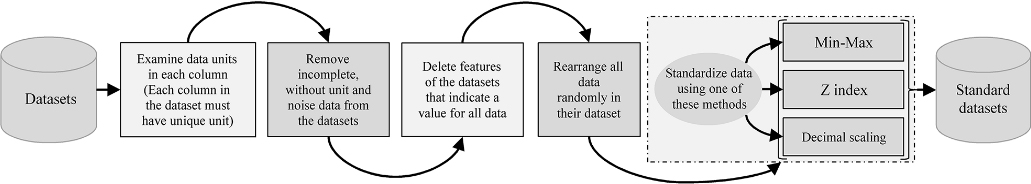

We use ten cancer and disease datasets taken from UCI datasets. In each dataset, about 20% of the data considered as test data and the rest of them as train data. We mention this number for understanding the relevant accuracies and indexes in Table 1. The number of data is in the range of 32 to 1040, and the number of features of the datasets is from nine to 69 features. There are also two, three and six classes of diseases. These intervals indicate that we focus on the significant number of datasets with different data and features; so, the results are sufficiently reliable. On the other hand, we use datasets with more than two classes of disease, so we evaluate our methods in the differential diagnosis and different disease groups. Table 1 presents some information about the selected datasets.

In the first step of data preparation, we examine the data units in each column so that each column in the dataset has a unique unit. Then, we remove all incomplete and without unit data from the datasets because of the classification methods used in this paper, which cannot work with incomplete data. However, there are other ways to solve missing and incomplete data problems, but we delete these data for learning classification methods with correct data and reducing the complexity of their learning method. We survived the noise data of each dataset as well. After deleting data with incomplete values and some noise data, we delete the features of the datasets that indicate a value for all data because these features do not contain semantics for classification methods, leading to additional operations and increased complexity.

Next, we rearrange all data randomly in each dataset because there were the same classes consecutively in some datasets. For example, assume that class of first 50 data in a dataset were all class 1 and second 50 data were all class 2; if we get first 20% of data for test data, then all of the test data have the same class and the accuracy of the classification method is not properly evaluated. In addition, this layout in a dataset occasionally led to wrong classification learning. Therefore, we mix different classes of a dataset using data rearrangement. In the fifth step, we standardize data with three methods include Z index, Min-Max, and decimal scaling. Then, we examine the standardized data and select the best standardization method for each dataset based on the correlation between the features and the data class. For most datasets, the Min-Max method is suitable because this method maintains the data behavior and makes it easier to work with the data (see Fig. 1).

After standardization, we apply feature reduction methods using PCA and Forward-backward feature selection method. Finally, we evaluate the results of this feature reduction method based on the accuracy and performances of the classification methods used herein.

4. A proposed feature reduction

Searching all subsets and orders for features is hard and time-consuming, especially for the dataset with a large number of features. Therefore, we use feature selection and feature reduction methods for decreasing complexity of computational results and increasing performances of other data mining methods. Every feature reduction and feature selection method considers a part of previous features and ignores other parts. Some of these methods pay attention to the value of features and some of them consider learning methods for evaluating resulting features. Therefore, their behaviors make different strengths and weaknesses for them. However, no method is best among feature selections and feature reductions. Therefore, we combine two different methods and create a proposed feature reduction method.

According to the literature review, feature selection methods are divided into three types based on their model and combination of selection algorithm:

•
Filter methods: These methods focus on general features like the correlation with the variables. They select features regardless of the model; for example, Fast Correlation-Based Filter (FCBF) is one of them and removes features highly correlated to each other for selecting features.
•
Wrapper methods: They consider a learning algorithm and evaluate subsets of features, unlike filter approaches, to detect the possible interactions between features.
•
Embedded methods: They try to combine the advantages of both previous methods. A learning algorithm takes advantage of its own feature selection process and performs feature selection and classification simultaneously.

Forward-backward feature selection is one of the wrapper methods. This feature selection has two steps, forward step, and backward step. If the forward step was more than the backward step, then it selects a number of features that make the best performances for learning algorithm and stores them. Next, it selects another number of features among stored features that the learning algorithm has better performances without them. If there is no any subset of feature that makes better performances for learning algorithm, feature selection stops, and stored features are accepted. If the forward step was smaller than the backward step, then it deletes a number of features that make the best performances for learning algorithm. Next, it selects another number of features among deleted features that the learning algorithm has better performances with them.

In the other hands, PCA is a feature reduction method that transforms the data to a new coordinate system such that the greatest variance by some projection of the data comes to lie on the first coordinate (called the first principal component), the second greatest variance on the second coordinate, and so on. The largest component selected in the PCA method has more value among different features, but it does not necessarily represent the most relevant feature for classifying different disease. PCA focuses on the value of features and ignores their effects on classification methods.

In the proposed feature reduction method, we use Forward-backward feature selection using NB as a learning algorithm. Then, we use PCA for finding a subset of features with more value. Therefore, the proposed feature reduction has the following steps:

(1) (1)
Select $X$ number of features among all features that make the greatest accuracy for NB and store them;
(2)
Delete $Y$ number of features among stored features that rest of them make better accuracy for NB;
(3)
Select $Z$ number of features among unstored features that make the greatest accuracy for NB that is more than previous accuracies and store them;
(4)
If there is no subset of features that make greater accuracy for NB, go to step 5, else go to step 2;
(5)
Apply PCA and keep a subset of features with the greatest eigenvalues that summation of them is more than 90% of summation of all eigenvalues.

$X$ , $Y$ and $Z$ are three integer numbers selected using Depth-first search algorithm for every dataset. $X$ is greater than $Y$ for all datasets and iterations of Depth-first search algorithm. NB is a classification method that considers the probability of features and has less complexity among other methods in this paper. Therefore, we use it as a learning algorithm of Forward-backward feature selection. The proposed feature reduction method has advantages of Forward-backward and PCA methods.
5. Classification methods

We use classification methods for disease diagnosis in this paper. Classification and regression are supervised-learning methods that match an instructional set of input-output pairs $\{{x_{n},t_{n}}\}_{n=1}^{N}$ where $x_{n}\in R^{M}$ . The output is $t_{n}\in{\cal R}$ in the regression problems and $t_{n}\in\mathbb{Z}$ in the classification problems. The main purpose is to find the suitable output $t^{*}$ for a new input data $x^{*}$ (see Fig. 2). We present more detail about NB, DT, KNN, CBR, RBF and SVM methods in the following.

Figure 2.

The structure of supervised learning problems.

5.1 Naïve bayesian method

The network structure of NB is a simple structure that the class or label node is the parent of other nodes. All features are independent in its structure, so we can find every feature probability according to independent conditional probability. Despite all the limitations, the effectiveness of NB is good even when the assumed independence among the features in most datasets is unrealistic because the independence of the features ignores any relationship between them.

5.2 Decision tree method

DT is a powerful tool for classifying and forecasting. The process of classifying for each instance in this method begins by evaluating the features expressed in the root node and then decreases the tree branches according to its value. This algorithm begins by selecting a test set that performs the best separation for the classes. In the next steps, the same steps done for other nodes with fewer data to create the best rules. There are different types of developed DT such as ID3, C4.5, CART, CHILD, and MARS. We use the C4.5 algorithm as DT in our paper.

5.3 K-nearest neighborhood method

KNN was very effective when faced with large educational collections in the 1960s, but it did not welcome widely until computational power increased. KNN learning methods are based on the analogy that comparing a set of tests with educational sets that are similar. Density or proximity defined using metric distance as Euclidean, Manhattan, Geodesic, etc. In this paper, we use Euclidean distance in the KNN method.

5.4 Case-based reasoning method

CBR is one of the decisions making methods that finds solutions for a problem by focusing on previous problem solutions in a particular domain. The basis of this approach is based on a principle that similar problems have similar solutions. Therefore, after finding solutions for previous problems similar to the new problem and adapting their solutions, we can find a suitable solution to the current problem. The criterion and standard used by this method to find similarities is an important feature. In this paper, we have taken the distance of data as the criterion.

5.5 Radial basis functions method

RBF is a type of neural networks that their processor units focused on radial basis functions. Its neural networks do not differ much from Multilayer perceptron networks in terms of general structure, but they differ in the type of processing that neurons perform on their inputs. However, its networks often have faster learning and preparation processes. In fact, it is easier to adjust its neurons because of neurons concentration on a specific functional range.

5.6 Support vector machine

We often pay attention to improve the structure of the neural network by minimizing estimation errors in neural networks such as multilayer perceptron and RBF. However, in a particular kind of neural network known as the SVM, we focus on reducing the operational risk. The structure of its network has many similarities to the multilayer perceptron neural network and practically the main difference is in the learning method. This method makes a linear superficial separator with maximum margins in a larger dimensional space. In other words, we can say that the margin of a linear classification is the smallest distance among all of the learning points on the superficial separator.

6. Reinforcing classification learning using clustering

Clustering methods are useful when we want to put data in some similar clusters and find suitable relationships. In clustering methods, we have a training dataset $\{x_{n}\}_{n=1}^{N}$ where $x_{n}\in R^{M}$ . The output is $t_{n}\in\mathbb{Z}$ and the goal is to find the suitable output $t^{*}$ for a new input data $x^{*}$ . In other words, we are looking for data clusters that have the same behavior in every cluster. We use dynamic clustering methods selection in our model for making better performances after classification. If we had a dataset with multi-group data, maybe classification cannot learn appropriate rules of all groups. Therefore, we use clustering before classification for increasing their performances. However, the clustering method can be useful for making better results; but it can make worse results if we use them without criterion and analyzing. For this purpose, we need to cluster our data according to the criterion that shows us the best method and number of clusters herein. In this paper, we find a suitable number of clusters for each method using the following criterion:

(Average distance of clusters centers or Separation – Average distance of the points within the clusters or Compactness)

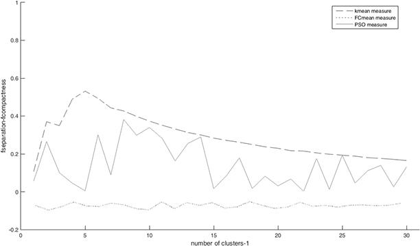
According to this criterion, the greater criterion is better and it presents a suitable number of clusters. We use K-means, Fuzzy Clustering (FC means) and Particle Swarm Optimization (PSO) as clustering methods. The number of studied clusters for each dataset is between one and $\text{round}({\sqrt{\text{number of data in a dataset}}})$ . We calculate the associated criterion for all number of clusters for every clustering method. Then, we select the maximum criterion; find the best clustering method and the number of its clusters.

Therefore, we find the best clustering method and the number of clusters according to the previous criterion. Next, we divide the data into train and test data groups, cluster data according to the best clustering method and find the train and test data in every cluster. Then, we learn every classification method with train data in each cluster, separately. When we want to predict the class of test data, we assign every test data to its cluster(s) and give it to the special classification method that learns related train data. Finally, we compare the calculated labels of test data and its main labels for finding accuracy. In this paper, we use the weighted mean for calculating classification accuracy according to the number of predicted data in every cluster.

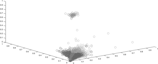
Table 2 presents two related figures for understanding previous steps. The first figure in this table presents defined criterion variations according to the number of clusters for every clustering method. According to the defined criterion, the higher criterion is better. The second figure in this table presents all data with the first third features of a dataset in the three-dimensional space.

Table 2
The output of clustering methods for one of the datasets

Summarily, we reduced the computation time of classification methods and their complexity using clustering and reducing the number of data for each train data. These methods have significant effects on classification performances.

7. The proposed multi-classifier method

According to previous steps, we make new datasets after data preparation, standardization, and applying the proposed feature reduction. Then, we use clustering methods and find the best clustering method among three clustering methods for every dataset and number of its clusters. We determine the cluster of every data and save it. Next, we select 80% of data as train data and consider them for making some rules. Rest of data are test data and the selection of test data is randomly in 10 different sets, so calculated accuracies are different for each random set. We use classification methods including NB, DT, KNN, CBR, RBF and SVM for train data of all clusters in every dataset and save their accuracy separately. These accuracies create some rules for the proposed MC. All accuracies are stored in the memory of MC. When we enter a test data to MC, it finds the cluster of this data and finds accuracies of classification methods related to this cluster. Then, it sorts these accuracies from high to low and identifies the best classification method among used classification methods. It is similar to proposed MC in the paper of Schapire [24], but there are different classification methods at previous step. The proposed MC selects one of them based on cluster of test data and accuracies of classification methods. According to samples in selected cluster, AdaBoost maintains a weight distribution over them. This distribution is uniform at first, but it updates based on following algorithm.

A set of training samples with labels $\{(x_{1},$ $y_{1}),$ $\ldots,$ $(x_{n},$ $y_{n})\}$ , a ComponentLearn algorithm, the number of cycles $T$ .

The weights of training samples: $w_{i}^{1}=1/N$ for all of $i=(1,\ldots,N)$ .

Do the following steps for $t=1,\ldots,T$ ;

•
Use the ComponentLearn algorithm to train a component classifier, $h_{t}$ , on the weighted training samples.
•
Calculate the training error of $h_{t}$ :

$\displaystyle\varepsilon_{t}=\sum^{N}_{i=1}w_{i}^{t}$ , $y_{i}\neq h_{t}({x_{i}})$ .
•
Set weight for the component classifier $h_{t}$ :

$\displaystyle\alpha_{t}={\displaystyle\frac{1}{2}}\ln\left({{\displaystyle% \frac{1-\varepsilon_{t}}{\varepsilon_{t}}}}\right)$ .
•
Update the weights of training samples:

$\displaystyle w_{i}^{t+1}={\displaystyle\frac{w_{i}^{t}\exp\{{-\alpha_{i}y_{i}% h_{t}({x_{i}})}\}}{C_{t}}}$ for all of $i=(1,\ldots,N)$ where $C_{t}$ is a normalization constant, and $\sum^{N}_{i=1}w_{i}^{t+1}=1$ .

$\displaystyle f(x)=\operatorname{sign}\left({\sum^{T}_{t=1}\alpha_{t}h_{t}(x)}\right)$ [24].

Figure 3.
Selected processes in this paper.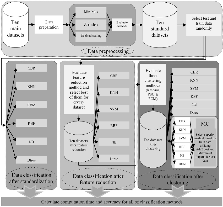

Obviously, the proposed algorithm is different for each cluster because of different selected classification method. ComponentLearn algorithm is adjusted based on this classification method. For example, we assume $\sigma$ and $\sigma_{\text{step}}$ as ComponentLearn algorithm for SVM and RBF [25], number of discrete probability ranges for NB, $\varepsilon^{t}$ and $\beta^{t}$ for DT [26]. However, if CBR or KNN classification methods are selected as best classification method, we use them together utilizing Mixture of Experts. Their weights are adjusted based on stored accuracies in MC memory. If FCmean was selected for a dataset and the test data belonged to several clusters, then MC considers its membership degree and the output of classification methods multiplied by the membership degree. After the aforementioned step, we round the answer for calculating label or class of data.

Finally, Fig. 3 shows all the steps used in this paper.

Table 3
The accuracy mean of classification methods

Classification methods Dataset 1 Dataset 2 Dataset 3 Dataset 4 Dataset 5 Dataset 6 Dataset 7 Dataset 8 Dataset 9 Dataset10 Average

Accuracy SVM 0.707 0.405 0.629 0.106 0.339 0.760 0.884 0.505 0.660 0.831 0.583

RBF 0.562 0.261 0.756 0.245 0.705 0.598 0.742 0.512 0.588 0.635 0.560

NB 0.461 0.262 0.768 0.369 0.566 0.681 0.722 0.374 0.415 0.254 0.487

KNN 0.551 0.219 0.803 0.125 0.509 0.367 0.673 0.850 0.341 0.813 0.525

Dtree 0.529 0.275 0.551 0.554 0.617 0.892 0.703 0.471 0.477 0.359 0.543

CBR 0.939 0.544 0.764 0.468 0.680 0.808 0.700 0.504 0.631 0.824 0.686

Accuracy after feature reduction SVM 0.993 0.681 0.911 0.586 0.806 0.996 0.902 0.989 0.784 0.987 0.863

RBF 0.970 0.663 0.882 0.438 0.800 0.936 0.806 0.968 0.765 0.896 0.812

NB 0.952 0.444 0.955 0.467 0.775 0.902 0.936 0.786 0.803 0.386 0.741

KNN 0.853 0.499 0.940 0.421 0.513 0.784 0.866 0.921 0.592 0.859 0.725

Dtree 0.982 0.480 0.955 0.725 0.781 0.904 0.781 0.913 0.797 0.763 0.808

CBR 0.974 0.682 0.950 0.752 0.739 0.912 0.752 0.942 0.838 0.907 0.845

Accuracy after feature reduction and clustering SVM 0.993 0.804 0.908 0.606 0.808 0.972 0.812 0.992 0.796 0.958 0.865

RBF 0.971 0.772 0.899 0.781 0.812 0.939 0.808 0.956 0.824 0.900 0.866

NB 0.951 0.593 0.956 0.804 0.786 0.909 0.948 0.905 0.902 0.455 0.821

KNN 0.840 0.572 0.937 0.466 0.550 0.861 0.930 0.928 0.668 0.792 0.754

Dtree 0.981 0.518 0.960 0.797 0.807 0.906 0.807 0.826 0.823 0.761 0.819

CBR 0.974 0.774 0.950 0.812 0.751 0.969 0.766 0.949 0.862 0.909 0.872

MC 0.993 0.810 0.963 0.824 0.811 0.984 1.000 0.989 0.895 0.971 0.924

Table 4
Accuracy variations for classification methods after modifying different train and test data for all datasets

Standard devariation of classification methods for 10 different seeds

Datasets SVM RBF NB KNN Dtree CBR MC

1 0.0081 0.0171 0.0263 0.0200 0.0295 0.0182 0.0083

2 0.0930 0.1139 0.0842 0.1535 0.2259 0.1257 0.0575

3 0.1276 0.0294 0.0220 0.0178 0.0119 0.0398 0.0105

4 0.1290 0.0447 0.0407 0.1137 0.1860 0.2346 0.0318

5 0.0617 0.0557 0.0414 0.0519 0.0851 0.1371 0.0543

6 0.0000 0.0902 0.1952 0.1178 0.1991 0.0511 0.0283

7 0.0000 0.0000 0.0279 0.0451 0.0000 0.0000 0.0000

8 0.0162 0.0748 0.0687 0.0417 0.1558 0.0665 0.0244

9 0.1759 0.0503 0.1168 0.1285 0.1084 0.0902 0.0531

10 0.0050 0.0469 0.2432 0.1135 0.2423 0.0486 0.0246

Mean 0.0617 0.0523 0.0866 0.0804 0.1244 0.0812 0.0293

8. Computational results

Classification methods	Dataset 1	Dataset 2	Dataset 3	Dataset 4	Dataset 5	Dataset 6	Dataset 7	Dataset 8	Dataset 9	Dataset10	Average
Accuracy	SVM	0.707	0.405	0.629	0.106	0.339	0.760	0.884	0.505	0.660	0.831	0.583
	RBF	0.562	0.261	0.756	0.245	0.705	0.598	0.742	0.512	0.588	0.635	0.560
	NB	0.461	0.262	0.768	0.369	0.566	0.681	0.722	0.374	0.415	0.254	0.487
	KNN	0.551	0.219	0.803	0.125	0.509	0.367	0.673	0.850	0.341	0.813	0.525
	Dtree	0.529	0.275	0.551	0.554	0.617	0.892	0.703	0.471	0.477	0.359	0.543
	CBR	0.939	0.544	0.764	0.468	0.680	0.808	0.700	0.504	0.631	0.824	0.686
Accuracy after feature reduction	SVM	0.993	0.681	0.911	0.586	0.806	0.996	0.902	0.989	0.784	0.987	0.863
RBF	0.970	0.663	0.882	0.438	0.800	0.936	0.806	0.968	0.765	0.896	0.812
NB	0.952	0.444	0.955	0.467	0.775	0.902	0.936	0.786	0.803	0.386	0.741
KNN	0.853	0.499	0.940	0.421	0.513	0.784	0.866	0.921	0.592	0.859	0.725
	Dtree	0.982	0.480	0.955	0.725	0.781	0.904	0.781	0.913	0.797	0.763	0.808
	CBR	0.974	0.682	0.950	0.752	0.739	0.912	0.752	0.942	0.838	0.907	0.845
Accuracy after feature reduction and clustering	SVM	0.993	0.804	0.908	0.606	0.808	0.972	0.812	0.992	0.796	0.958	0.865
RBF	0.971	0.772	0.899	0.781	0.812	0.939	0.808	0.956	0.824	0.900	0.866
NB	0.951	0.593	0.956	0.804	0.786	0.909	0.948	0.905	0.902	0.455	0.821
KNN	0.840	0.572	0.937	0.466	0.550	0.861	0.930	0.928	0.668	0.792	0.754
Dtree	0.981	0.518	0.960	0.797	0.807	0.906	0.807	0.826	0.823	0.761	0.819
CBR	0.974	0.774	0.950	0.812	0.751	0.969	0.766	0.949	0.862	0.909	0.872
	MC	0.993	0.810	0.963	0.824	0.811	0.984	1.000	0.989	0.895	0.971	0.924

	Standard devariation of classification methods for 10 different seeds
Datasets	SVM	RBF	NB	KNN	Dtree	CBR	MC
1	0.0081	0.0171	0.0263	0.0200	0.0295	0.0182	0.0083
2	0.0930	0.1139	0.0842	0.1535	0.2259	0.1257	0.0575
3	0.1276	0.0294	0.0220	0.0178	0.0119	0.0398	0.0105
4	0.1290	0.0447	0.0407	0.1137	0.1860	0.2346	0.0318
5	0.0617	0.0557	0.0414	0.0519	0.0851	0.1371	0.0543
6	0.0000	0.0902	0.1952	0.1178	0.1991	0.0511	0.0283
7	0.0000	0.0000	0.0279	0.0451	0.0000	0.0000	0.0000
8	0.0162	0.0748	0.0687	0.0417	0.1558	0.0665	0.0244
9	0.1759	0.0503	0.1168	0.1285	0.1084	0.0902	0.0531
10	0.0050	0.0469	0.2432	0.1135	0.2423	0.0486	0.0246
Mean	0.0617	0.0523	0.0866	0.0804	0.1244	0.0812	0.0293

We used Matlab R2015a (8.5.0.197613) 64-bit software on a personal computer with Intel (R) Core (TM) i3-2120 CPU @ 3.30GHz processor and 4.00 GB RAM for all runs. We use 10 random sets of train and test data for evaluating classification methods. Table 3 presents the accuracy mean of them.

Table 5
The computation time mean of classification methods

Classification methods		Dataset 1	Dataset 2	Dataset 3	Dataset 4	Dataset 5	Dataset 6	Dataset 7	Dataset 8	Dataset 9	Dataset10	Average
Computation time	SVM	8.582	4.306	5.330	4.516	4.593	38.559	4.058	1.219	2.161	2.956	7.628
Computation time	RBF	3.575	4.155	5.236	0.383	1.566	6.554	0.354	0.204	0.980	4.517	2.752
	NB	3.834	0.189	2.938	4.620	0.688	0.555	2.547	3.384	3.939	4.933	2.763
	KNN	4.447	4.330	0.947	0.651	3.119	5.021	0.239	2.581	4.994	0.300	2.663
	Dtree	2.065	3.667	2.515	3.045	1.492	1.580	3.775	4.466	3.236	1.130	2.697
	CBR	2.912	4.170	5.732	2.408	4.920	6.301	2.853	3.910	2.004	2.813	3.802
Computation time after feature reduction	SVM	7.150	0.072	2.414	1.119	0.879	38.401	1.080	0.172	0.375	0.782	5.244
	RBF	1.297	0.082	3.759	0.130	0.204	2.394	0.140	0.089	0.105	0.185	0.838
	NB	0.056	0.017	0.030	0.005	0.018	0.074	0.005	0.004	0.005	0.049	0.026
	KNN	0.416	0.009	0.863	0.044	0.081	0.921	0.036	0.013	0.022	0.081	0.249
	Dtree	0.613	0.236	0.521	0.237	0.263	0.503	0.223	0.208	0.229	0.372	0.340
	CBR	2.215	0.030	2.407	0.146	0.355	4.943	0.157	0.068	0.100	0.454	1.087
Computation time after feature reduction and clustering	SVM	14.62	0.120	70.651	3.391	1.552	73.363	0.964	0.283	0.449	1.249	16.664
	RBF	1.025	0.186	2.573	0.826	0.401	3.177	0.868	0.568	0.438	0.263	1.032
	NB	0.961	0.083	2.483	0.281	0.632	2.299	0.254	0.082	0.137	0.694	0.791
	KNN	1.119	0.016	3.721	0.215	0.219	3.963	0.178	0.057	0.074	0.142	0.970
	Dtree	0.936	0.477	3.389	2.208	0.883	1.794	2.172	1.470	1.200	0.626	1.516
	CBR	7.403	0.029	24.339	0.540	1.080	28.047	0.595	0.133	0.233	0.843	6.324
	MC	71.61	0.262	202.720	8.566	5.784	942.006	9.545	1.910	2.563	2.521	124.749

According to Table 3, the accuracy mean of CBR is better than other classification methods after standardization (68%). Next, we use the proposed feature reduction and it improves classification accuracies. The most improvement belongs to SVM (28%) and it has the best accuracy mean (86%) as well. Then, we use clustering for improving previous results. All classification methods present better accuracy means and MC has the best accuracy mean among them (92%). In addition, CBR has better accuracy among rest of classification methods (87%).

Figures 4–6 are related to first, second and third part of Table 3 and present more details about accuracy mean variations of classification methods.

Figure 4.

Accuracy mean of different classification methods for every dataset.

Figure 5.

Accuracy mean of different classification methods for every dataset after feature reduction.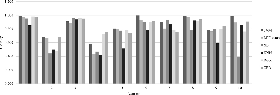

Figure 6.

Accuracy mean of different classification methods for every dataset after feature reduction and clustering.

We use 10 random sets of train and test data for evaluating the performances of the classification methods in different datasets. Table 4 presents standard devariations for accuracies of classification methods. According to Table 4, MC has the least accuracy mean variations with random sets.

In Table 5, we present the computation time of classification methods for different datasets.

According to Table 5, the computation time mean of KNN is better than other classification methods after standardization (2.66). Next, we use the proposed feature reduction and it decreases all classification computation times. The most improvement belongs to NB (2.74) and it has the best computation time mean (0.02) as well. Then, we use clustering for improving accuracies. It increases their accuracy and computation time means. NB has the best computation time mean among them after clustering (0.79).

9. Conclusion

Every classification method has certain strengths and weaknesses. We can improve its performances using some methods but they cannot improve all of their weaknesses. In this paper, we combine Forward-backward feature selection and PCA feature reduction methods and present a proposed feature reduction method that increases accuracy and decreases computation time of all used classification methods. In addition, we use three clustering methods for dividing the datasets into smaller datasets in order to simplify the classification learning process and increase accuracy. Then, we present the MC classification method that takes advantages of all used classification methods in this paper. We evaluate and compare the performances of different classification methods based on ten disease-related datasets from the UCI website according to accuracy, computation time and variations of accuracies for different test and train datasets. We use 10 random different sets of train and test data for every dataset.

According to our computational results, we conclude that CBR has the best accuracy mean (68%) and KNN has best computation time mean (2.66) after standardization. Next, we use the proposed feature reduction and it improves all classification accuracies and computation times. The most improvement in accuracy belongs to SVM (28%) and it has the best accuracy mean (86%) as well. However, the most improvement in computation time belongs to NB (2.74) and it has the best computation time mean (0.02) as well. Then, we use clustering for improving previous results. All classification methods present better accuracy means. MC has the best accuracy mean among them (92%) and the least accuracy mean variations with random sets. In addition, CBR has better accuracy among rest of classification methods (87%). It is noteworthy that NB has the best computation time mean among classification methods after clustering (0.79).

The proposed MC presents good results for differential diagnosis in datasets with more than two disease classes. Therefore, it is a very useful method for designing a decision support system for the aforementioned cancers and diseases. Based on our extensive computational results, we believe that the proposed MC can reduce physicians’ decision errors and the cost of medical care.

References

Sboner

Eccher

Blanzieri

Bauer

Cristofolini

Zumiani

, et al. A multiple classifier system for early melanoma diagnosis. Artificial Intelligence in Medicine. 2003; 27(1): 29-44.

Binder

Schwarz

Winkler

Steiner

Kaider

Wolff

, et al. Epiluminescence microscopy: A useful tool for the diagnosis of pigmented skin lesions for formally trained dermatologists. Archives of Dermatology. 1995; 131(3): 286-291.

Bischof

Talbot

Breen

Lovell

Chan

Stone

, et al. Automated melanoma diagnosis system. 1999; 3747: 130-141.

Daskalakis

Kostopoulos

Spyridonos

Glotsos

Ravazoula

Kardari

, et al. Design of a multi-classifier system for discriminating benign from malignant thyroid nodules using routinely H&E-stained cytological images. Computers in Biology and Medicine. 2008; 38(2): 196-203.

Peng

. A novel ensemble machine learning for robust microarray data classification. Computers in Biology and Medicine. 2006; 36(6): 553-573.

Hayashi

Setiono

. Combining neural network predictions for medical diagnosis. Computers in Biology and Medicine. 2002; 32(4): 237-246.

Polat

Gunes

. A novel hybrid intelligent method based on C4.5 decision tree classifier and one-against-all approach for multi-class classification problems. Expert Systems with Applications. 2009; 36(2): 1587-1592.

Nanni

. Letters: An ensemble of classifiers for the diagnosis of erythemato-squamous diseases. Neurocomputing. 2006; 69(7): 842-845.

Polat

Gunes

. The effect to diagnostic accuracy of decision tree classifier of fuzzy and k-NN based weighted pre-processing methods to diagnosis of erythemato-squamous diseases. Digital Signal Processing. 2006; 16(6): 922-930.

10.

Das

. A comparison of multiple classification methods for diagnosis of Parkinson disease. Expert Systems With Applications. 2010; 37(2): 1568-1572.

11.

Das

Turkoglu

Sengur

. Effective diagnosis of heart disease through neural networks ensembles. Expert Systems With Applications. 2009; 36(4): 7675-7680.

12.

Woniak

Grana

Corchado

. A survey of multiple classifier systems as hybrid systems. Information Fusion. 2014; 16: 3-17.

13.

Yin

Jha

. A health decision support system for disease diagnosis based on wearable medical sensors and machine learning ensembles. 2017; 3(4): 228-241.

14.

Beevi

Nair

Bindu

. A multi-classifier system for automatic mitosis detection in breast histopathology images using deep belief networks. IEEE Journal of Translational Engineering in Health and Medicine. 2017; 5: 1-11.

15.

Chen

Dou

Wang

Qin

Heng

. Mitosis detection in breast cancer histology images via deep cascaded networks. 2016; 1160-1166.

16.

Tek

. Mitosis detection using generic features and an ensemble of cascade adaboosts. Journal of Pathology Informatics. 2013; 4(1): 12-12.

17.

Wang

Cruzroa

Basavanhally

Gilmore

Shih

Feldman

, et al. Cascaded ensemble of convolutional neural networks and handcrafted features for mitosis detection. Proceedings of SPIE. 2014; 9041.

18.

Veta

Diest

Pluim

. Detecting mitotic figures in breast cancer histopathology images. Proceedings of SPIE. 2013; 8676: 867607.

19.

Dalvi

Vernekar

. Anemia detection using ensemble learning techniques and statistical models. 2016; 1747-1751.

20.

Lan

Gao

. A new model of combining multiple classifiers based on neural network. 2013; 154-159.

21.

Bashir

Qamar

Khan

Javed

. An efficient rule-based classification of diabetes using ID3, C4.5, a CART ensembles. 2014; 226-231.

22.

Kim

Cho

. Ensemble bayesian networks evolved with speciation for high-performance prediction in data mining. 2017; 21(4): 1065-1080.

23.

Fei

Shuan

Yan

Xiaoning

King

. Prediction on customer churn in the telecommunications sector using discretization and Naïve Bayes classifier. International Journal of Advances in Soft Computing & Its Applications. 2017; 9(3).

24.

Schapire

Singer

. Improved boosting algorithms using confidence-rated predictions. 1998; 37(3): 80-91.

25.

Wang

Sung

. AdaBoost with SVM-based component classifiers. Engineering Applications of Artificial Intelligence. 2008; 21(5): 785-795.

26.

Quinlan

. Bagging, boosting, and C4.S. 1996; 725-730.

An efficient multi-classifier method for differential diagnosis

Abstract

Keywords

1. Introduction

2. Literature review

Table 1 Used datasets

4. A proposed feature reduction

5.2 Decision tree method

5.3 K-nearest neighborhood method

5.4 Case-based reasoning method

5.5 Radial basis functions method

5.6 Support vector machine

6. Reinforcing classification learning using clustering

Table 2 The output of clustering methods for one of the datasets

Table 5 The computation time mean of classification methods

References

Table 1
Used datasets

Table 2
The output of clustering methods for one of the datasets

Table 5
The computation time mean of classification methods