Comparative investigation of machine learning algorithms for detection of epileptic seizures

Abstract

In modern day Psychiatric analysis, Epileptic Seizures are considered as one of the most dreadful disorders of the human brain that drastically affects the neurological activity of the brain for a short duration of time. Thus, seizure detection before its actual occurrence is quintessential to ensure that the right kind of preventive treatment is given to the patient. The predictive analysis is carried out in the preictal state of the Epileptic Seizure that corresponds to the state that commences a couple of minutes before the onset of the seizure. In this paper, the average value of prediction time is restricted to 23.4 minutes for a total of 23 subjects. This paper intends to compare the accuracy of three different predictive models, namely – Logistic Regression, Decision Trees and XGBoost Classifier based on the study of Electroencephalogram (EEG) signals and determine which model has the highest rate of detection of Epileptic Seizure.

Keywords

Epileptic seizures electroencephalogram (EEG) signals logistic regression decision trees XGBoost classifier true positive prediction rate preictal state prediction time

1. Introduction

Neurological disorders have been on the rise in the past few decades at an alarming rate and affect millions of people worldwide every year. Neurological disorders are the diseases that are responsible for the breakdown of the human nervous system that includes the nerves, spinal cord and the brain. Alzheimer’s, epilepsy, migraine etc. are a few of the most prominent of the diseases. Among them, Epilepsy [1] is the neurological disorder that is the number two most prevailing in the world. As per the WHO, more than 50 million people all across the globe are affected by epilepsy and 6 million deaths per year are caused by stroke. Thus, it is clear that epileptic seizures are a major neurological health concern throughout the world. Although there is no cure that can treat epilepsy permanently, there are various methods through which health experts detect and diagnose epilepsy.

Epilepsy can be recognised by the sudden seizures [2] experienced by the patient without any warnings that leave the patient convulsing, cause muscle pain and spasms and lose consciousness. Epilepsy is most prominent in the elderly over the age of 65 but is also commonly seen in children who show autistic behaviour. It has also been found that people with certain genes are more susceptible to epilepsy, though finding relations between genes of brain and epilepsy is very complex and in fact, not possible at all for some forms of epilepsy. Another common cause of epilepsy is an infection in the brain. Curing such infections often results in the formation of scars inside the brain and makes the person more prone to epilepsy. Epilepsy can be categorised into four types based on the type of seizure one experiences. They are namely: Generalised epilepsy, Focal Epilepsy, Generalised and Focal epilepsy and Unknown Epilepsy. Generalised epilepsy affects a major portion of the brain’s electrical signals and often causes unconsciousness. Focal epilepsy is epilepsy that only affects a certain portion of the brain. The third category is where the patient has both of the epilepsies together. Unknown epilepsy is the type where it is known that the patient has seizures but the type of epilepsy cannot be determined.

Past studies about application of AI in detection of emotion, heart rate and Parkinson’s disease [3, 4, 5] have shown that no method exists which guarantees the hundred percent successful detection of any disease using machine learning technique as within every proposed method there may exists some form of errors. Hence, there exist wide variety of parameters and their combination which can be used for reliable seizure detection and therefore need for finding the most accurate models and selecting features which yield best results will be always there. Thus, this study aims to test the accuracy by training and testing sample dataset of 178 features of EEG signal, using same dataset to test and compare different machine learning models so as to find algorithms having highest AUC score and finally to test the how different learning method i.e., logistic regression, ensemble learning and tree-based method performs for these kinds of detections.

For this study, the predictive analysis of the dataset is done by deploying specific prediction models, that are studied under the domain of Machine Learning. Machine Learning has similar origins as to the field of AI and is used to make systems perform tasks that they are not exclusively programmed for. Machine learning has various applications in AI, designing of digital control systems and, as in this case, prediction and forecasting. The main contributions of authors are as follows.

•
The paper aims to devise a method to detect the occurrence of an epileptic seizure by training machine learning [6] algorithms using a sample dataset of 178 features of the EEG signals [7].
•
The Extreme gradient boost method is proposed for detection of epileptic seizure with improved accuracy.
•
The results of the proposed technique have been compared with Logistic Regression and Decision trees for investigation of its effectiveness.

The paper has been organised in the following sections – Related work tells the research and experimental work that has been done until now. In this section, different methods have been used which are broadly classified into linear and non-linear techniques and the different number of features, channels, their combinations along with different processing and pre-processing procedures and different ML algorithms have been used for classification.
2. Dataset

The dataset that is taken into consideration for carrying out the predictive analysis is taken from the UCI Machine Learning Repository. The data corresponds to multivariate time series data, comprising of a total of 178 features, that are observed over one categorical variable, for a total of 11,500 number of instances. In the dataset, every numerical value corresponds to a neurological pulsating voltage signal of different degrees that are recorded at different instantsof time. The dataset comprises of five different classes of data, depicted by classes – A, B, C, D, E, each class consisting of 100 single-channel EEG signalsegments, that are recorded for a total time duration of 23.4 seconds. For the classes A and B, different segments of EEG signals were recorded for a total of five neurologically healthy persons by deploying the scheme of placing the standard electrode. In the case of class A, it was ensured that people are in a conscious state ensuring that their eyes were opened, while in class B, the people were conscious making sure that their eyes were closed. For the classes C, D and E, the data is recorded in archived format by performing the presurgical diagnosis of the EEG signals. This data is recorded in the case of five different patients, who were subjected to complete control of the seizures and subsequent diagnosis of theirzone of epilepsy was performed. In the case of class C, the data was collected during the formation process of Hippocampal on the opposite hemisphere of the neurological brain, while the class D of data was recorded during the zone of Epilepsy [34].

It is to be noted that the data taken into consideration has been pre-processed and reorganised, in reference to the original dataset on the UCI online machine learning repository [35]. Each class of data – A, B, C, D and E are represented in digital format, in the form of 4097 different data points. These data points are furthermore divided into 23 different chunks of data whose distribution is performed along 178 time – feature readings of neurological voltage pulsating signals. Henceforth, creating 5 different classes of data for 100 individual EEG signal data segments leads to the creation of 11,500 instances of data. The distribution of data in chunks of 23 data elements refers to the fact that 23 different electrodes are deployed during the recording process of the EEG signals.

From this, we derive an attribute that represents the output in the form of different classes.

Class 5: Class 1:
For these patients, the recording of the EEG signals was performed during the activity of seizures, corresponding to Ictal data.
Class 2:
In this case, the data elements are recorded from the zone of Epilepsy of the patient’s brain and subsequently, tumours are identified.
Class 3:
This class corresponds to the patients for whom, the data elements are recorded from the non-epileptic part or the healthy part of the brain in achieved formats and subsequent tumours are detected and located.
Class 4:
It is used to represent healthy people who are acting as volunteers (data class – B), for whom, the EEG signal activity is recorded in perfectly normal conditions with their eyes closed.
Class 5:
This class represents healthy people serving as a volunteer (data class – A), and for those, the activity of the EEG signals is recorded in a perfectly normal environment with their eyes open.

It should be noted that the data is recorded in a time-series or time-stamp format, corresponding to neurological pulsating voltage signals, depicted in the unit of microvolts. These signals are recorded at different time instances in correspondence to 178 different attributes. After performing meticulous exploration of the raw dataset, it was discovered that there were no missing elements in the dataset.
3. Related work

As discussed in the previous section, the onset of the epileptic seizures can be predicted a few minutes before the onset of seizures based on the Electroencephalography of the person concerned. This prediction is done by studying the neural activity of the brain with the help of recordings taken from Electroencephalography (EEG) combined with the Machine learning techniques.

Electroencephalography (EEG) is a monitoring method to study the electrophysiological activity of the brain. It records the electrical activity of the brain non-invasively by measuring the voltage fluctuations due to the flow of ionic current within the neural mesh. The voltage difference from the two sides of the brain is recorded over time and graphically displaced representing a proportional measure of activity. The EEG data is represented as a continuous-time series waveform representing the voltage fluctuations in microvolts. Though the recording is taken by placing small metal plates as electrodes on the surface of the brain, the waveforms recorded are influenced by neural activities going deep within the cortex [23].

The Electrodes are placed at specifically designated parts of the scalp and the recordings are measured with respect to the reference electrodes placed individually or preconfigured cap. With the invent of Analog to digital converter these analogue signals can now be recorded, displaced and processed for further evaluation. These digital machines give an edge over the conventional analogue machines as they are useful only for continuous pattern analysis, moreover, the waveform generated is displaced in the groups [24, 25].

The ionic potential across the neural membranes is responsible for normal neural activity. The potential across the diffusion membrane exist due to the efflux of potassium ion to establish the electrochemical equilibrium. This membrane potential resulting from the electrophysiological activity of the brain give rise to brain waves. These brain waves are recorded by the Electroencephalography (EEG) [22, 23]. The signal generated hasa sinusoidal waveform witha peak-to-peak voltage having a magnitude of 0.5 up to 100 microvolts in the healthy human brain. These waves are grouped into four categories viz. 1) Delta: 0.5 to 4 Hz, 2) Theta: 4 to 8 Hz, 3) Alfa: 8 to 13 Hz and 4) Beta: all greater than 13 Hz [20, 21].

EEG has a wide span in clinical application and Epilepsy being the most common one [21]. Interpretation of EEG is a highly complex process involving multi-disciplinary expertise and involves many decision-making steps [21]. It is due to the fact that a similar pattern may result due to different reasons or unrelated patterns may indicate the same reason. Irregular EEG pattern may or may not indicative of epileptic seizures.

EEG pattern in an epileptic seizer can be categorised into four stages viz. 1) The preictal state, the state which is a precursor to the onset of a seizure, 2) The ictal state, the second state that coincides with the onset of a seizure, 3) The postictal state, it is the state that comes after the ictal stateand 4) Interictal state, the state that starts after the end of postictal of first seizures and ends before the onset of the preictal state of second seizures.

Table 1
Comparison of machine learning models for the prediction of epileptic seizures

Models	Number of seizures	Number of subjects	Number of features	EEG Channel used	False positive rate	Average sensitivity (%)
Bandarabadi et al. [23]	87	24	12	6	0.06	73.98
Gadhoumi et al. [24]	86	6	3	02/03	0.15	88.00
Rasekhi et al. [25]	86	10	22	6	0.17	71.97
Teixeira et al. [26]	87	224	22	6	0.33	73.08
Zandi et al. [27]	86	20	18/23	18/23	0.155	88.34

The detection of the preictal state gives us sufficient time before the seizure occurs. It starts some moments before the onset of seizure [26]. For this purpose, many researchers have tried classification for differentiating the preictal and the ictal state, Pre-processing of EEG signal with an aim to increase SN ration and use the use of modern techniques like feature extraction plays a vital role in reliable prediction. Various researchers have tried to combine multiple features into a feature vector with an aim to improve the models.

In the recent literature we can find references to various seizure detection method that are broadly categorized into five linear domains such as frequency domain [36], time-domain [37], EMD – empirical mode decomposition [38], wavelet domain (time-frequency) [39], and rational transform domain [40] and other non-linear domains such as HOS – higher-order spectra [41], information theory and entropy [42], Lyapunov exponent [43], and intrinsic mode functions (IMF) [44] for detecting epileptic seizures through EEG signals analysis using Machine learning (ML) frameworks. Non-linear methods have shown higher potential in detecting epileptic seizures rather linear methods since EEG are known to have more non-linear feature.

Whereas other literature hadtried to use a different number of features, channels, different methods and different ML algorithms, such as spectral power features [26], wavelet method [27], univariate linear features extraction [28], expansion of features [29], zero-crossing technique [30].

It has been observed through the comparative study of different researches that, there is no reliable method for selection of channels and EEG signal processing. Table 1 shows a comparative view of various methods, machine learning models trained on the basis of different number of seizures, number of subjects, Number of features, EEG Channel, type of EEG data, false-positive rates, average sensitivity.

4. Methodology

The Data is collected for processing through the method of EEG, or Electroencephalography [9]. EEG refers to the process of observing the electrical signals generated by human brain when millions of neurons fire up simultaneously at a particular part of the brain and in a similar rhythm or pattern. This electrical activity of the brain that has recognisable behavioural pattern is usually associated with certain body actions and thus can be processed to predict the response of the body in advance. Electroencephalography records these signals in the form of the amplitude of their voltage.

Normally, this electrical activity of the brain shows a similar pattern for most of the people and only differs in case of any abnormality in the body or brain. Hence detecting these unusual patterns in brain activity can help in identifying the various neurological disorders that a person may be afflicted with. The paper proposes a method of using the EEG as inputs to predicting the chances of a seizure at any given time by using machine learning, specifically, logistical regression, decision tree and extreme gradient boosting. The aim is to use these techniques to successfully predict the occurrence of a seizure and observe the accuracy of prediction to find the best possible technique of all the ones discussed here. The relevant theory regarding the working of the three techniques is discussed below.

The input signals received from the EEG are processed in the time domain [10] and then passed through the predictor model for analysis. It gives valuable information like features with the most impact on the occurrence of a seizure, the true and false positive rates and their area under the curve, etc. that are then used for feature selection and judging the accuracy of the models. The graphical representation of methodology is shown in Fig. 1.

Figure 1.

Steps for detection of epileptic seizures.

One of the benefits of using the extreme gradient boost is that it has the important functionality of feature selection. What it does is that it allots a score to all the features that tell how important that feature is in ascertaining the output. The score is calculated by the amount of increase in performance due to the attribute split point for each decision tree and multiplied by the number of observations for that particular node. Then the average of this score is taken over all the decision trees.

The overall accuracy [11] of the prediction is judged by finding out the true and false positive rates and carrying out further calculations [12]. The true positive rate signifies the rate of the correct affirmative predictions that are made by the model whereas the false positive rate tells the rate of incorrect affirmative predictions made by the model.

Accuracy can then be found out using this data. Accuracy can be defined as ratio of correct observations to all the observations made by the model. In this case, as per definition:

$\displaystyle\text{Accuracy}=\text{Correct predictions}/\text{All Predictions}$

This can be further divided based on the nature of the prediction whether it is affirmative or negative:

$\displaystyle\text{Accuracy}={(\textit{Tp}+\textit{Tn})}/{(\textit{Tp}+\textit% {Tn}+\textit{Fp}+\textit{Fn}})$ (2)

where $\textit{Tp}=$ True Positive; $\textit{Tn}=$ True Negative; $\textit{Fp}=$ False Positive; $\textit{Fn}=$ False Negative.

Figure 2.

Positive feature importance score – XGBoost Classifier.

The value of accuracy always is less than 1, or equal to 1 in the case of 100% accuracy, which is practically highly unlikely and may be due to overfitting. Also, while useful, the accuracy alone does not give us the full picture of the performance of the prediction model. There might be the case when only one type of true value (either positive or negative) may have a good prediction but the other not so good. But accuracy alone won’t be able to detect this. Hence, we use multiple different approaches [9] to ensure the best results. One such method is finding the AUC (Area Under the Curve) and ROC (Receiver Operating Characteristics) respectively [14]. Positive feature importance score is presented for XGBoost model in Fig. 2.

Figure 3.

ROC prediction curve.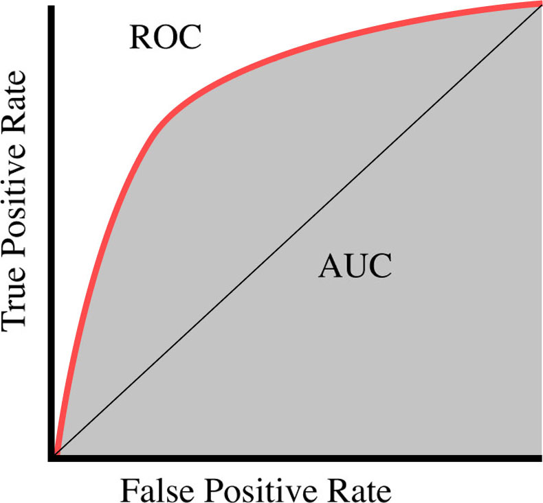

This AUC-ROC curve is used for analysing the performance of the classification techniques in various stages, represented for proposed work in Fig. 3. A higher value of AUC means that the model can differentiate between the different classes much more sharply. This is especially useful for binary classification problems.

Some defining features of the curve are:

$\displaystyle\textit{True Positive Rate/Recall}=\textit{Tp}/{(\textit{Tp}+% \textit{Fn})}$ (3) $\displaystyle\textit{Specificity}=\textit{Tn}/{(\textit{Tn}+\textit{Fp})}$ (4) $\displaystyle\textit{False Positive rate}=1-\textit{Specificity}$ (5) $\displaystyle\textit{False Positive rate}={\textit{Fp}}/{(\textit{Tn}+\textit{% Fp})}$ (6)

The model which has AUC of 1 is considered to be an accurate one, whereas the model with AUC of 0.5 is considered the worst. Interestingly, the model that has AUC of 0 means that it is complementing the actual output, that is, the prediction is the opposite of the true value in all the cases.

4.1 Logistic regression (as a classifier)

Logistic regression [15] is a machine learning technique whose objective in our paper is to perform binary classification of data. Binary classification means dividing data into two classes. For example, for testing a patient to be diabetic or not we denote a patient being diabetic by 1 or 0 for not diabetic. Thus 2 classes are denoted here by 1 and 0. Now by using the logistic regression algorithm we are training our machine learning model and trying to classify data in either of the two classes as accurately as possible.

Logistic regression is similar to linear regression technique as they both are used to perform classification. The significant differences between the two lies in the way they both model the data. In Logistic regression, the data is modelled as binary values whereas in linear regression the data is modelled as a continuous numeric value. Another key difference is, in the case of linear regression there is a linear relationship between dependent and independent variables whereas there is no such dependency in logistic regression. Linear regression uses a straight line to classify data whereas logistic regression uses sigmoidal function [16] to do the classification.

Linear Regression

$\displaystyle Y=A_{0}+A_{1}*W_{1}+A_{2}*W_{2}+\ldots+A_{k}*W_{k}$

where, $Y$ is the log of odds, $W_{1},W_{2},\ldots,W_{k}$ are independent variables, $A_{0},A_{1},\ldots,A_{k}$ are the coefficient of inputs.

Sigmoid Function

$\displaystyle P=\frac{1}{1+e^{-y}}$ (8)

where, $P$ is a probability function, $y$ is the log of odds.

Usually, Logistic regression performs better than linear regression in solving classification problems especially when there are outlier points in the dataset. These outlier points may affect the overall prediction accuracy of linear regression.

Figure 4 above is a sample of the logistic regression model [17].

Figure 4.

Logistic regression model.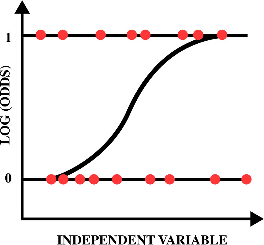

4.2 Logistic regression algorithm

1.
Calculate the weighted sum of inputs by using the equation below:

$\displaystyle Y=mw+c$ (9)

Here, $Y$ is dependent variable, $W$ is independent variable.

This $Y$ represents log of odds* [18].

$\displaystyle\textit{Odds}=\frac{P}{1-P}$ (10)

where $P$ represents the probability of an event to occur.
2.
Now we need to find the probability of a person having a seizure which is given by substituting the value of the log of the odds in the sigmoidal function given below:

$\displaystyle P=\frac{1}{1+e^{-y}}$ (11)
3.
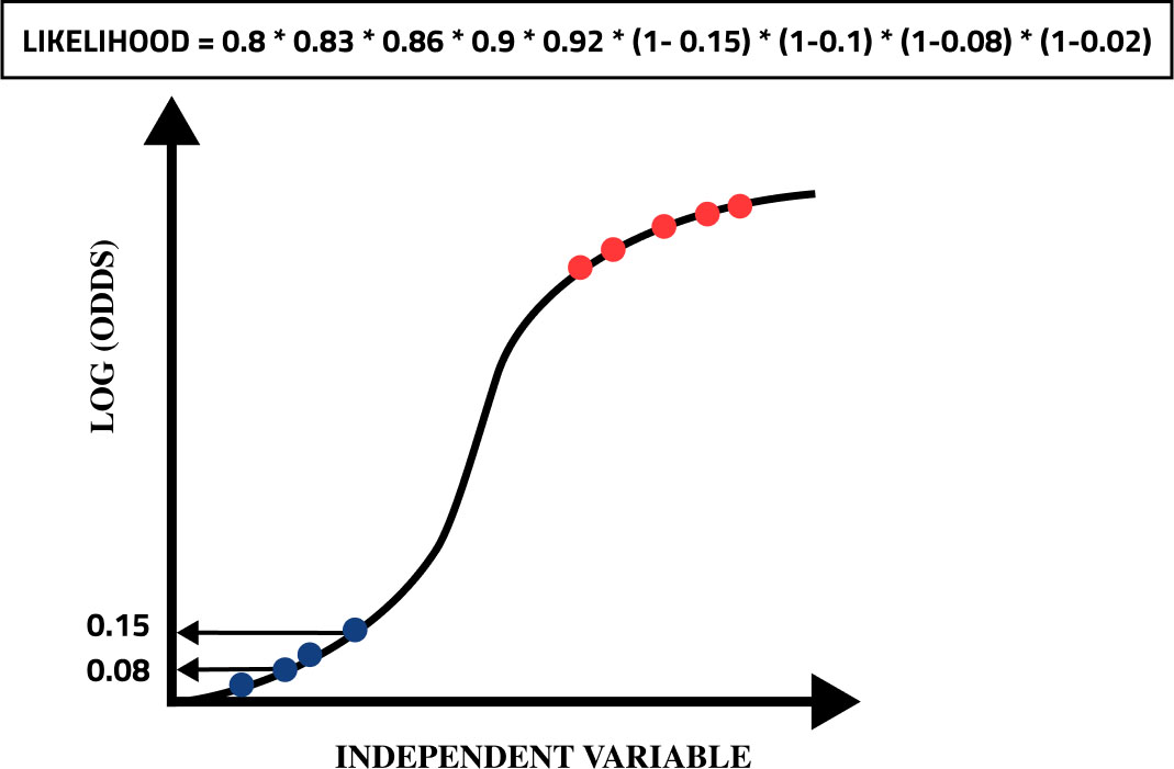
Now after finding the probabilities of a person having a seizure or not, we need to select a sigmoidal function that best fits our data. For this, we need to train our machine learning model using techniques like Gradient Descent, Maximum likelihood etc.
4.
In maximum likelihood technique, we include the chances of people who have a seizure and those who don’t have a seizure.

The value of likelihood is found by the product of each value.

Figure 5.
Denoting likelihoods of people.

Figure 6.
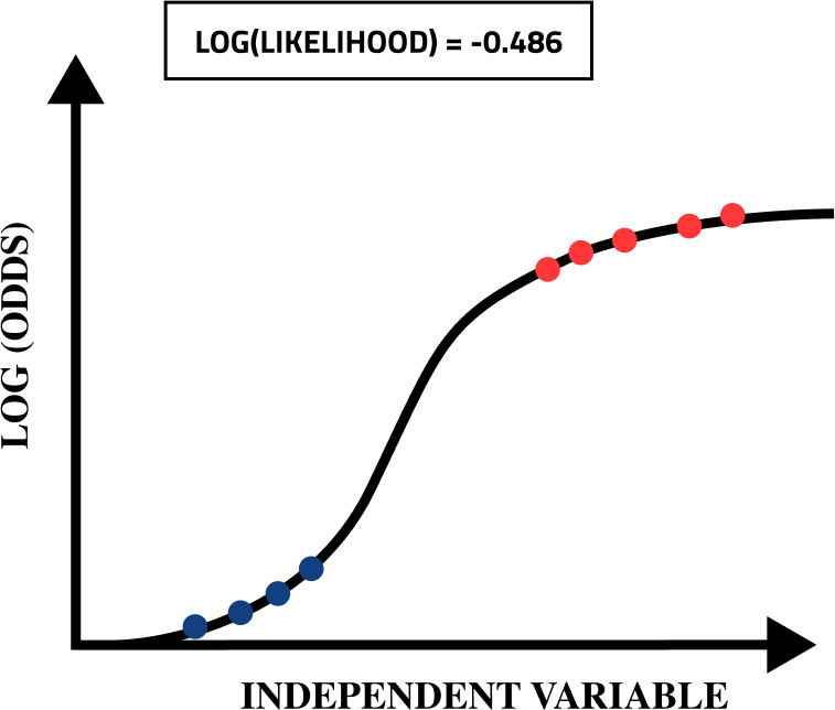
Value of likelihood for a particular line.

On taking Log of the likelihood we end up with the following likelihood, presented in Figs 5 and 6.
5.
We will keep on repeating the entire process for different lines and find the value of likelihood for each line. The line which is providing the maximum value of likelihood is chosen.
6.
Upon training the logistic regression model using the maximum likelihood technique, we can check the accuracy of the model by calculating the errors after predicting the data of some people having epilepsy or not.

4.3 Decision tree

Decision Tree [36] is a modern classification algorithm implemented in the domain of Machine Learning and Data Science based on the Supervised Learning Algorithmic Model. This algorithm can be deployed to solve modern computational problems that involve predicting data trends with the help of advanced Regression and Classification techniques. The core structure depicting this algorithm resembles the structure of a tree comprising of different nodes. All these nodes in a Decision Tree are used to describe a statement pertaining to a certain condition. Interconnection of these nodes is made possible with the help of branches, which serve the purpose of depicting the results to the statements represented by the decision tree nodes. The execution of the algorithm commences from the topmost node, also known as the Root node, and finishes when the execution reaches the Bottom-most node, also known as the Leaf Node. Once all the attributes pertaining to the upper nodes are executed, the final decision made by the algorithm is represented by the Leaf Node. In this sense, the Leaf node is also called the Terminal Node. In comparison to conventional Machine Learning Algorithms, this technique is significantly preferable in terms of parameters like algorithmic accuracy and algorithmic stability and its interpretation in comparison to other techniques is far easier. Diagrammatical representation is given in Fig. 7.

Figure 7.

Diagrammatic representation of a decision tree.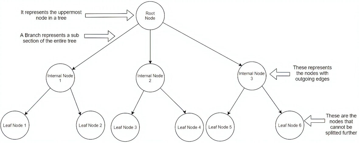

Steps involved in building a Decision Tree model [36] are as follows:

The first step of the building process involves a meticulous inspection of the dataset and based on that, deciding which elements of the dataset can be considered as the Root Node of the decision tree.

The second step deals with dividing the dataset into different subsets to create subsequent datasets that are available for training and testing the algorithm.

The third step involves validating that every single subset should depict homogenous values corresponding to every individual element.

The last step of the building process involves the repeated execution of the aforementioned steps until the Terminal Nodes corresponding to all the branches of the decision tree is determined. Henceforth, the nodes at the terminal depicts the Predicted values.

4.4 XGBoost classifier

Extreme Gradient boost also known as XGBoostis a highly efficient and scalable implementation ofthe gradient boosting package. The XGBoost offers better scalability and has the capability to perform parallel and distributed computing offering faster learning and model exploration. This newly introduced package offers various objective functions including Ranking, Classifier and Regression.

With its advantage of adjustable parameters, XGBoost can make predictions on the set of defined standard features and offers better results than other machine learning models. The package contains a linear model and tree learning algorithm [32].

Figure 8.

XGBoost algorithm as an implementation of gradient boosted decision tree.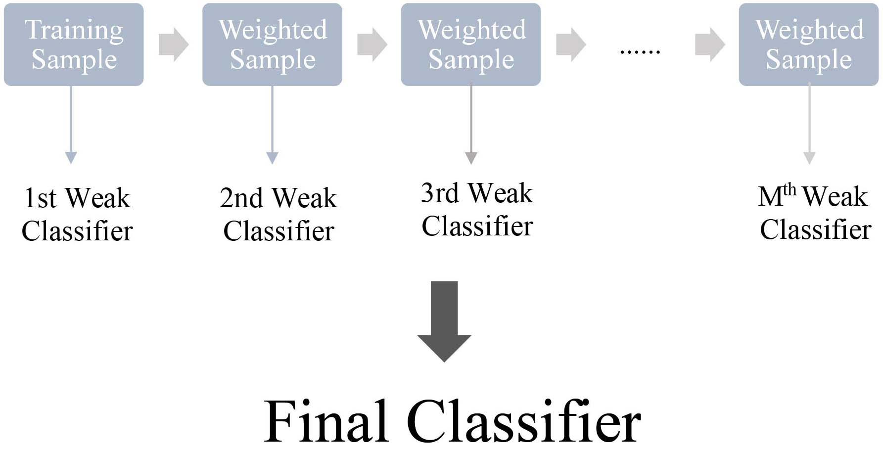

XGBoost is based ensemble learning method, which generates an ensemble model by the iterative cycle of predictions as presented in Fig. 8. In this model, a naive model is used to start the cycle as we need initial predictions. Even if these predictions are wildly inaccurate, subsequent cycles can address these errors. To make predictions, predictions from all the previous models are used to build a new model [33].

New predictions are based upon the model having previously added predictions. These predictions are then used to calculate errors, build into a model and added to the ensemble. These iterations are performed until the residuals from the previous model are reduced as much as possible. Figure 9 depicts the flow chart for XGBoost model.

Figure 9.

Flow Chart representing XGBoost algorithm.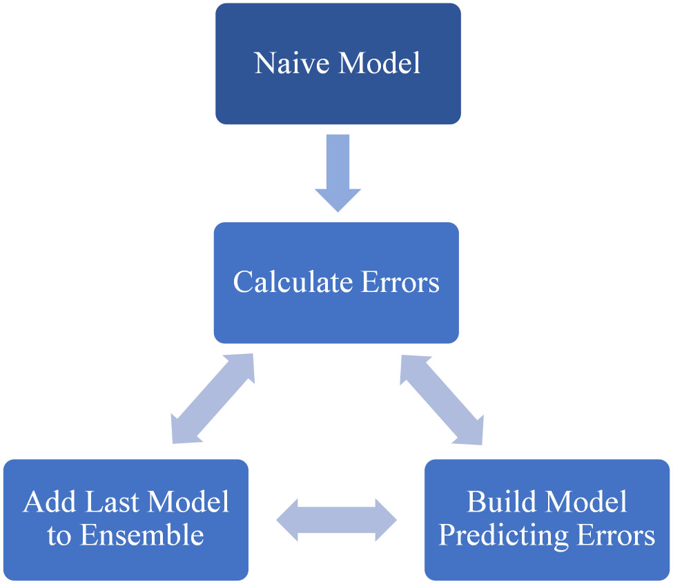

Figure 10.

AUC Score comparison for 3 different classification techniques.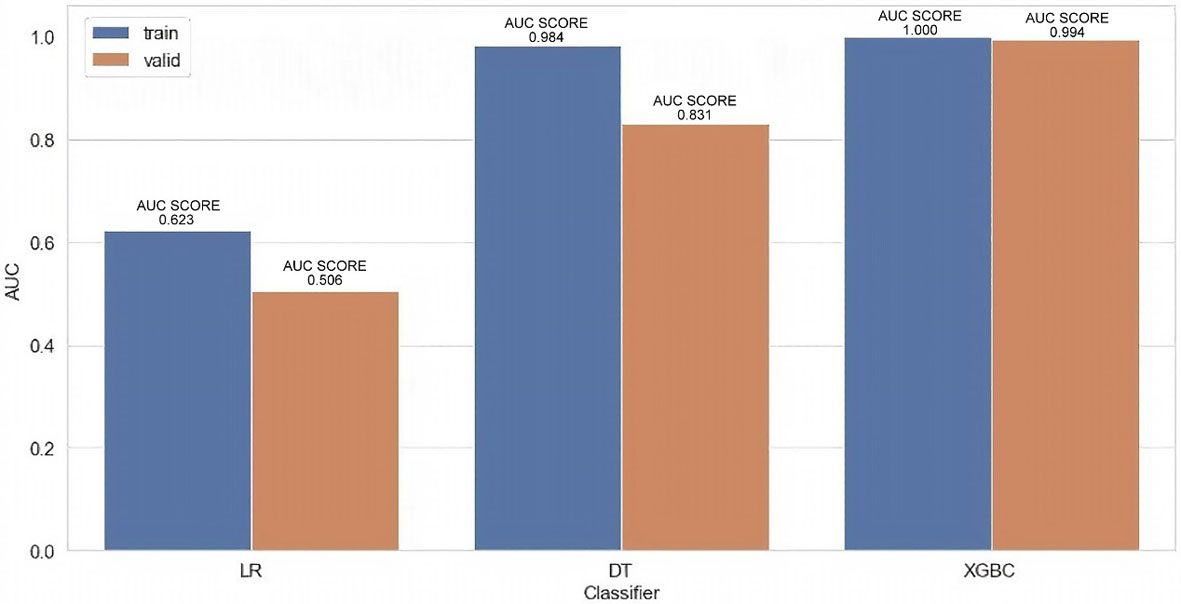

Figure 11.

ROC Curve for XGBoost classification algorithm.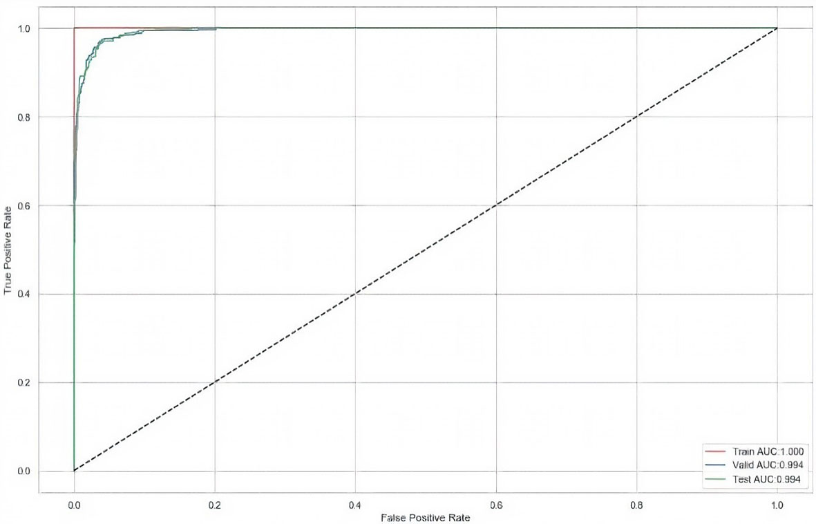

There are three stems in boosting using ensemble learning technique:

•

A target variable $y$ is predicted based upon an initially defined model $F_{0}$ . This model will be associated with a residual $(y-F_{0})$ .

•

A new model $h_{1}$ is fit to the residuals from the previous step

•

Now, $F_{1}$ a boosted version of $F_{0}$ is built upon $F_{0}$ and $h_{1}$ . $F_{1}$ will have a lower mean squared error than that from $F_{0}$ :

$\displaystyle F_{1}(x)\to F_{0}(x)+h_{1}(x)$ (12)

The residuals of $F_{1}$ are used to create a new model $F_{2}$ to further enhance the performance of $F_{1}$ :

$\displaystyle F_{2}(x)\to F_{1}(x)+h_{2}(x)$ (13)

We try to minimise the residual as much as possible by performing iterations up to $m$ cycle:

$\displaystyle F_{m}(x)\to F_{m-1}(x)+h_{m}(x)$ (14)

The functions created in previous models do not get disturbed by the additive learners. Instead, they impart information to bring down the errors.

Here, $F_{0}(x)$ is the initially defined model, $F_{1}(x),$ $F_{2}(x),\ldots,F_{m-1}(x)$ are the intermediate model, $F_{m}(x)$ is the final model in $m^{\text{th}}$ cycle, $h_{1}(x)$ is theinitial regression tree which tries to reduce the residuals from the previous step, $h_{2}(x),h_{3}(x),\ldots,h_{m-1}(x)$ are the regression tree in intermediate cycle, $h_{m-1}(x)$ is the final regression tree which along with $F_{m-1}(x)$ is used to create final model $F_{m}(x)$ .

5. Results

The results of different binary classification algorithms are depicted with the help of AUC Scores for different classification techniques. AUC Scores are significant when it comes to the analysis of different classification techniques due to the fact that they represent the degree of separability of the algorithm. In other words, it tells the degree up to which the classification model is correctly able to distinguish between different classes.

The Fig. 10 represents the AUC score comparison for 3 different binary classification techniques, namely – Logistic Regression (as a classifier), Decision Tree classifier and XGBoost Classifier. For better analysis, the dataset is divided into 2 separate subsets of data – Training Data and Validation Data. For both these subsets of data, it is visible that the XGBoost Classification technique produces the highest value of the AUC score, thus depicting a higher degree of separability.

Table 2 shows a comparative view of AUC scores of the training data and validation data for Logistic Regression, Decision Tree classifier and XGBoost Classifier.

Table 2
AUC score of the training and validation data for different machine learning models used

Models	AUC scores of the training data	AUC scores of the validation data
Logistic regression	0.623	0.506
Decision tree classifier	0.984	0.831
XGBoost classifier	1.000	0.994

The ROC (Receiver Operating Characteristic) as shown in Fig. 11, Curve is plotted between two algorithmic parameters namely, the True Positive Rate and False Positive Rate for a specified classification technique. The area under this curve is calculated for determining the AUC Score of a classification algorithm. In the above figure, the ROC curve is plotted for the XGBoost Binary Classification Algorithm. The AUC scores obtained for the Training, Validation and Testing Datasets are 1.00, 0.994 and 0.994 respectively. From this information, we can infer that the XGBoost Classification algorithm is 99.4% correct in the prediction of the positive classes in the testing dataset.

6. Conclusion

This paper entails the accuracy of the predictive models namely XGBOOST, LR and DT for the detection of epileptic seizures based on the study of EEG signals. In the proposed work, XGBOOST model have been implemented to analyse the EEG readings and automatically classify the patient as having epilepsy or not. The results of XGBOOST have compared with LR and DT model for investigation of effectiveness of the proposed method. In the case of classification problems, we have compared the classification ability of different ML techniques using AUC score. Technique which is having more AUC score is said to have better classification ability. On comparing the AUC score of all the techniques, we concluded that XGBoost is the best technique to classify the given data with the AUC score 0.994. This study can be extended in future by using extra tree classifier, addition of more parameters and implementation latest machine learning techniques for improving the accuracy to detect epilepsy.

References

De Lucia

Fritschy

Dayan

Holder

. A novel method for automated classification of epileptiform activity in the human electroencephalogram-based on independent component analysis. Med Biol Eng Comput. 2008; 46: 263-272. doi: 10.1007/s11517-007-0289-4.

Hamad

Houssein

Hassanien

Fahmy

. A hybrid EEG signals classification approach based on grey wolf optimizer enhanced SVMs for epileptic detection. in: International Conference on Advanced Intelligent Systems and Informatics (Cairo). 2017; 108-117.

Saxena

Tripathi

Khanna

Gupta

Sundaram

. Emotion detection through eeg signals using FFT and machine learning techniques. in: International Conference on Innovative Computing and Communications. Advances in Intelligent Systems and Computing. Khanna

Gupta

Bhattacharyya

Snasel

Platos

Hassanien

, eds, 2020; 1087. Springer, Singapore. doi: 10.1007/978-981-15-1286-5_46.

Prerna

Krishna

Kshitij

Rahul

Deepak

Arun

. Artificial plant optimization algorithm to detect heart rate & presence of heart disease using machine learning. Artificial Intelligence in Medicine. 2020; 102: 101752. doi: 10.1016/j.artmed.2019.101752.

Goel

Khanna

Gupta

. Detection of parkinson’s disease using machine learning techniques for voice and handwriting features. in: International Conference on Innovative Computing and Communications. Advances in Intelligent Systems and Computing. Khanna

Gupta

Bhattacharyya

Snasel

Platos

Hassanien

, eds, 2020; 1087. Springer, Singapore. doi: 10.1007/978-981-15-1286-5_56.

Ahmedt-Aristizabal

Fookes

Nguyen

Denman

Sridharan

Dionisio

. Deep facial analysis: A new phase I epilepsy evaluation using computer vision. Epilepsy Behav. 2018; 82: 17-24. doi: 10.1016/j.yebeh.2018.02.010.

Iasemidis

Shiau

Pardalos

Chaovalitwongse

Narayanan

Prasad

, et al. Long-term prospective on-line real-time seizure prediction. Clin Neurophysiol. 2005; 116: 532-544. doi: 10.1016/j.clinph.2004.10.013.

Yuan

Zhou

Liu

Wang

. Epileptic seizure detection with linear and nonlinear features. Epilep Behav. 2012; 24: 415. doi: 10.1016/j.yebeh.2012.05.009.

Wilson

Scheuer

Emerson

Gabor

. Seizure detection: Evaluation of the reveal algorithm. Clin Neurophysiol. 2004; 115: 2280-2291. doi: 10.1016/j.clinph.2004.05.018.

10.

Chen

Xie

Bui

Krzyżak

. Automatic epileptic seizure detection in EEG using nonsubsampled wavelet-fourier features. J Med Biol Eng. 2017; 37: 123-131. doi: 10.1007/s40846-016-0214-0.

11.

Ullah

Hussain

Qazi

EUH

Aboalsamh

. An automated system for epilepsy detection using eeg brain signals based on deep learning approach. Exp Syst Appli. 2018; 107: 61-71. doi: 10.1016/j.eswa.2018.04.021.

12.

Shoeb

Guttag

. Application of machine learning to epileptic seizure detection. in: International Conference on Machine Learning (Haifa). 2010; 975-982.

13.

Pachori

Patidar

. Epileptic seizure classification in EEG signals using second-order difference plot of intrinsic mode functions. Comput Methods Programs Biomed. 2014; 113: 494-502. doi: 10.1016/j.cmpb.2013.11.014.

14.

Quintero-Rincón

Pereyra

, D’ Giano

Batatia

Risk

. A new algorithm for epilepsy seizure onset detection andspread estimation from EEG signals. Journal of Physics: ConferenceSeries. 2016; 705(1): 012032.

15.

Fisher

Acevedo

Arzimanoglou

Bogacz

Cross

Elger

Forsgren

French

Glynn

Hesdorffer

Lee

Mathern

Moshe

Perucca

Scheffer

Tomson

Watanabe

Wiebe

. ILAE official report: A practical clinical definition of epilepsy. Epilepsy. 2014; 55(4): 475-482.

16.

Bishop

. Pattern recognition and machine learning. Springer-Verlag New York Hosmer

Lemeshow

Sturdivant

. Applied logistic regression. Wiley; 2013.

17.

Alkan

Koklukaya

Subasi

. Automatic seizure detection in EEG using logistic regression and artificial neural network. Journal of Neuroscience Methods. 2005; 148: 167-176.

18.

Bhowmick

Abdou

Bener

. Predictive analytics in healthcare epileptic seizure recognition. in: Proceedings of the 28th Annual International Conference on Computer Science and Software Engineering. 2018; 323-330. IBM Corp.

19.

Benbadis

. Abnormal nonepileptiform EEG. in: Handbook of EEG Interpretation, second ed. Demos Medical Publishing, New York, USA. 2014; 2: 51-70.

20.

Martinerie

Adam

Le Van Quyen

Baulac

Clemenceau

Renault

Varela

. Epileptic seizures can be anticipated by non-linear analysis. Nature Medicine. 1998; 4: 1173-1176.

21.

Niedermeyer

Lopes da Silva

. Electroencephalography: Basic principles, clinical applications, and related field, fifth ed. Lippincott Williams and Wilkins, Philadelphia, USA; 2005.

22.

William

Tatum

Normal

EEG

. In Handbook of EEG Interpretation, second ed. Demos Medical Publishing, New York, USA. 2008; 1: 1-50.

23.

Chernecky

Berger

. Laboratory tests and diagnostic procedures, six ed. Elsevier Health Sciences, USA; 2013.

24.

Teplan

. Fundamentals of EGG measurement. Measurement Science Review. 2002; 2(2): 1-11.

25.

Usman

Fong

. Epileptic seizures prediction using machine learning methods. Computational and Mathematical Methods in Medicine; 2017.

26.

Bandarabadi

Teixeira

Rasekhi

Dourado

. Epileptic seizure prediction using relative spectral power features. Clinical Neurophysiology. 2015; 126(2): 237-248.

27.

Gadhoumi

Lina

Gotman

. Discriminating preictal and interictal states in patients with temporal lobe epilepsy using wavelet analysis of intracerebral EEG. Clinical Neurophysiology. 2012; 123(10): 1906-1916.

28.

Rasekhi

Mollaei

MRK

Bandarabadi

Teixeira

Dourado

. Preprocessing effects of 22 linear univariate features on the performance of seizure prediction methods. Journal of Neuroscience Methods. 2013; 217(1-2): 9-16.

29.

Teixeira

Direito

Bandarabadi

. Epileptic seizure predictors based on computational intelligence techniques: A comparative study with 278 patients. Computer Methods and Programs in Biomedicine. 2014; 114(3): 324-336.

30.

Zandi

Tafreshi

Javidan

Dumont

, Predicting epileptic seizures in scalp EEG based on a variational bayesian gaussian mixture model of zero-crossing intervals. IEEE Transactions on Biomedical Engineering. 2013; 60(5): 1401-1413.

31.

Chen

Benesty

Khotilovich

Tang

. Xgboost: Extreme gradient boosting. R package version 0.4-2. 2015; 1-4.

32.

Chen

Guestrin

. Xgboost: A scalable tree boosting system. in: Proceedings of the 22nd Acmsigkdd International Conference on Knowledge Discovery and Data Mining. 2016; 785-794.

33.

Andrzejak

Lehnertz

Mormann

Rieke

David

, and Elger, CE. Indications of nonlinear deterministic and finite-dimensional structures in time series of brain electrical activity: Dependence on recording region and brain state. Physical Review

. 2001; 64(061907): 1-8.

34.

University of California Irvine. Epileptic Seizure Recognition DataSet. https://archive.ics.uci.edu/ml/datasets/Epileptic+Seizure+Recognition; 2017.

35.

Song

. Decision tree methods: Applications for classification and prediction. Shanghai archives of psychiatry. 2015; 27(2): 130-135. doi: 10.11919/j.issn.1002-0829.215044.

36.

Bhople

Tijare

. Fast Fourier transform based classification of epileptic seizure using artificial neural network. Int J Adv Res Comput Sci SoftwEng. 2012; 2(4).

37.

Shanir

Khan

Farooq

. Time domain analysis of EEG for automatic seizure detection. in: National Conference on Emerging Trends in Electrical and Electronics Engineering (ETEEE-2015); 2015.

38.

Huang

Shen

Long

Shih

Zheng

Yen

Tung

Liu

. The empirical mode decomposition and the Hilbert spectrum for nonlinear and non-stationary time series analysis. Proceedings of the Royal Society of London. Series A: Mathematical, Physical and Engineering Sciences. 1998; 454(1971): 903-995. doi: 10.1098/rspa.1998.0193.

39.

Polat

Ozerdem

. Epileptic seizure detection from EEG signals by using wavelet and Hilbert transform. in: 2016 XII International Conference on Perspective Technologies and Methods in MEMS Design (MEMSTECH). 2016; 66-69. IEEE. doi: 10.1109/MEMSTECH.2016.7507522.

40.

Samiee

Kovacs

Gabbouj

. Epileptic seizure classification of EEG time-series using rational discrete short-time Fourier transform. IEEE transactions on Biomedical Engineering. 2014; 62(2): 541-552. doi: 10.1109/TBME.2014.2360101.

41.

Acharya

Sree

Ang

PCA

Yanti

Suri

. Application of non-linear and wavelet based features for the automated identification of epileptic EEG signals. International Journal of Neural Systems. 2012; 22(2): 1250002. doi: 10.1142/S0129065712500025.

42.

Chai

Zou

. Hilbert marginal spectrum analysis for automatic seizure detection in EEG signals. Biomedical Signal Processing and Control. 2015; 18: 179-185. doi: 10.1016/j.bspc.2015.01.002.

43.

Faust

Acharya

Adeli

. Wavelet-based EEG processing for computer-aided seizure detection and epilepsy diagnosis. Seizure. 2015; 26: 56-64. doi: 10.1016/j.seizure.2015.01.012.

44.

Kumar

Sriraam

Benakop

Jinaga

. Entropies based detection of epileptic seizures with artificial neural network classifiers. Expert Systems with Applications. 2010; 37(4): 3284-3291. doi: 10.1016/j.eswa.2009.09.051.

Comparative investigation of machine learning algorithms for detection of epileptic seizures

Abstract

Keywords

1. Introduction

Table 1 Comparison of machine learning models for the prediction of epileptic seizures

Table 2 AUC score of the training and validation data for different machine learning models used

References

Table 1
Comparison of machine learning models for the prediction of epileptic seizures

Table 2
AUC score of the training and validation data for different machine learning models used