A parallel feature selection algorithm for detection of cancer biomarkers

Abstract

Biomarker plays an important role in early disease diagnosis including cancer. The World Health Organization defines a biomarker as any structure or process in the body that is measurable and affects the prognosis or outcome of the disease. Today, biomarkers can be identified using bioinformatics tools. The detection of biomarkers in the field of bioinformatics is considered more as a problem of feature selection. Many feature selection algorithms have been used for biomarker discovery however these algorithms do not have enough accuracy or have computational complexity. For this reason, the researchers discard the high accuracy algorithms because they are time consuming. We redesigned an efficient algorithm based on parallel algorithms. We used the Cancer Genome Atlas (TCGA) including breast cancer patients. The proposed algorithm has the same accuracy and increases the speed of algorithm.

Keywords

Biomarker bioinformatics breast cancer parallel algorithm MSVM-RFE

1. Introduction

Any matter, structure, or process that is measurable in the body and can affect the prediction or trend of the disease is known as a biomarker [1, 2]. Biomarkers can diagnose the disease before clinical symptoms appear, so it is vital to use them in early detection of diseases [3]. The discovery of cancer biomarkers results in the early detection of cancer, which will have a significant impact on the mortality rate of the disease. Biomarkers are obtained from the analysis of biomolecules such as DNA, RNA and proteins and can themselves be proteins, genes, hormones and enzymes [4].

The discovery of biomarkers is a matter of feature selection in bioinformatics, especially when the distinction between features is important [5]. Feature selection means finding a subset of attributes with the minimum possible size that contain the necessary information for the intended purpose. In the biomarker detection problem, we also encounter a large number of features and samples. The goal is to select a subset of the minimal features that are very close and efficient to the examples. The feature selection algorithms, in addition to returning a set of features as output, reduce the dimension and the redundancy of data and increase the accuracy [6]. With the help of these algorithms, it is possible to identify and validate biomarkers in several steps. First, the needed genomic and proteomic data is collected and organized by databases. In addition, unnecessary data is deleted. The second step involves feature selection and, in some cases, use classification methods. Appropriate tools should validate the candidate biomarkers at a later stage [7].

1.1 Feature selection algorithms

Feature selection algorithms can be grouped into three categories: filter, wrapper, and embedded. Filter approach work based on the inherent nature of the data. These types of algorithms are usually simple and do not have high computational complexity. However, these algorithms are not very accurate and usually not stable. It means, for each execution, it usually returns different attributes [8]. An example of these algorithms is the Relief algorithm that is unstable and has been used for the detection of biomarkers [9]. Wrapper algorithms use classification methods for ranking features. Wrapper algorithms have high computational complexity and are not sufficiently fast, but due to using classification, the relationships between features are considered and algorithms are highly accurate [8]. One of the most widely used algorithms for biomarker discovery is subset that was used as a wrapper algorithm [10]. Because this algorithm has constraints as a feature selection algorithm, a combination of this algorithm and a recursive feature elimination algorithm (SVM-RFE)1

¹
SVM-RFE: Support Vector Machine - Recursive Feature Elimination.

was proposed. This algorithm has increased the accuracy of its previous algorithms [11]. Since then, the SVM-RFE was considered as a benchmark algorithm for other feature selection classification [12].

Feature selection algorithms generally have different performances on different data types in terms of biology [8]. In addition, due to the growing amount of data in biology area, the choice of fast algorithms has priority. Only the filter algorithms with this data volume can return the output at an acceptable time. As stated, these algorithms do not have the required precision in detecting cancer biomarkers, while misinterpreting biomarkers can cause many problems [8]. The use of wrapper algorithms is now increasing rapidly due to the high accuracy but the computational complexity of these algorithms and their running time is significant [12]. One of the main solutions to reduce the computational complexity of algorithms is the parallelization method. Parallelization means increasing the number of processors and dividing the work or data into several sub-tasks so, the calculations are divided between the processors and the response time is reduced [13, 14].

2. Proposed parallel SVM-RFE

The SVM-RFE algorithm is one of the best feature selection algorithms for biomarker detection and is considered by many researchers in this field. This algorithm is stable, meaning that the output of the algorithm is constant at each repeat. It also has good accuracy in detecting biomarkers, and it is very time-consuming just because of the use of a support vector machine algorithm [15, 16]. This algorithm performs very well on genomic data [12]. In this paper, first, the dataset is introduced then the parallelization method for this algorithm is described.

2.1 Data source

The Cancer Genome Atlas (TCGA) is a large dataset of genomic variation in more than 33 types of cancer, which is valuable for computing tools. This dataset contains the genomic changes, DNA sequences, and gene expression in a cell tumor relative to a healthy cell. This study covers gene expression for more than a thousand patients with breast cancer and includes the expression of genes, metabolism, and clinical data for 2012–2015 [15]. By integrating these collections, the number of samples is more than 1,800 patients and the number of features is more than 2000 features. This data consists of rows as samples (patients) and columns show features. The second column is the patient’s status, which consists of two modes: live or dead, that plays the role of the tag. In fact, we are looking for biomarkers that play the biggest role in survival or death.

2.2 mSVM-RFE

In 2005, a different implementation of the SVM-RFE algorithm was introduced which at each step instead of one support vector machine, it uses several support vector machines [16]. This algorithm was known as a tool to select the effective genes in cancer classification and it returned better features than the SVM-RFE algorithm. In addition, the quality of the classifier is better [16]. Due to using several classes at the classification stage, this algorithm was called the mSVM-RFE algorithm.

The algorithm receives the data from the user, then $k$ -Fold method is used to create sub-samples randomly. The user with $k$ variable introduces the number of these subsamples. In the second step, the support vector machines (the number is specified by the user) are trained on each subsample, and the value of each feature is estimated using all machines. Each machine has its weight vector and for each property such as $i$ , let $w_{j,i}$ be the weight of the $i^{\text{th}}$ feature in $j^{\text{th}}$ SVMs [15]:

$\displaystyle vj,i=\left({w_{j,i}}\right)^{2}$

And the ranking score for each feature such as $i$ , is defined as:

$\displaystyle ci=\frac{v_{i}}{\sigma_{i}}$ $\displaystyle v_{i}=\frac{1}{t}\mathop{\sum}\limits_{j=1}^{t}\left({w_{j,i}}% \right)^{2}$ $\displaystyle\sigma_{i}=\sqrt{\frac{\mathop{\sum}\nolimits_{j=1}^{t}\left({v_{% j,i}-v_{i}}\right)^{2}}{t-1}}$

Figure 1.

The proposed parallel algorithm.

In the next step, the feature with the smallest ranking is eliminated. The second and third steps are repeated until for all features, their ranking be calculated. In the end, five (or more) features with the highest ranking are returned as an output [16]. In this algorithm, as in SVM-RFE, in each iteration, we can eliminate several features instead of one by one.

This algorithm is more expensive than the SVM-RFE algorithm because it uses multiple SVMs instead of one machine. However, this cost will ultimately lead to a better feature selection and more accurate ranking. In addition, one of the ways that we can increase the stability of algorithms is to select the features on different subsets [16]. Both algorithms were performed on the breast, lung, colon, and blood dataset and the best features for breast cancer and blood cancer were obtained by mSVM-RFE. On colon cancer, the selected features by SVM-RFE were better [16].

2.3 Parallelization method

We used R studio in this research implemented the mSVM-RFE algorithm in R [17]. There are several libraries for parallelism in R that the most important is the Rmpi library [18]. Suppose that $k=$ 10 for the $k$ -Fold function. It means we have 10 subsamples of data. The user determines the number of SVMs ( $t$ ). If $t=$ 1, SVM-RFE will be executed, if $t>$ 1, mSVM-RFE will be executed. The larger number increases the accuracy. However, the complexity will also increase significantly. With $k$ subsamples and $t$ linear SVMs, ( $k*t$ ) machines will be executed in each iteration [16].

In the first step, the $k$ -fold function divides data into subsamples. Therefore, we do not need to split data from the beginning. Then we scatter folds to processors, and then each process executes the other steps of the algorithm. The number of subsamples in parallel mode should be set based on the number of processors. If our computer uses four simultaneous processors so, the number of subsamples will be a multiple of 4. If there are 8 subsamples, each of the processors will get two subsamples. Therefore, at each step of mSVM-RFE, the number of linear SVMs altogether is:

$\displaystyle t\left(\textit{svm}\right)\ast k\left(\textit{fold}\right)=t\ast k$

In general, the time complexity of algorithms in the recursive part will be as follows:

$\displaystyle\left(\mathop{\sum}\limits_{i=0}^{m}\left({t\ast k}\right)\right)% \ast n=O\left({\left({m\ast t\ast k}\right)\ast n}\right)$

Where $m$ is the number of features and $n$ is the number of samples.

Suppose that we have $p$ processor. The dataset is partitioned into $k$ folds and each processor has one or more folds. Therefore, in this case, we have data parallelism. Furthermore, each processor runs $t$ machines on its folds. It means the linear SVMs $\left({t\ast k}\right)$ are distributed on different processors:

$\displaystyle\left[\sum_{i=0}^{m}\left(\frac{t\ast k}{p}\right)\right]\ast% \frac{n}{p}=O\left(\!\!\left(m\ast\frac{t\ast k}{p}\right)\!\ast\!\left(\frac{% n}{p}\right)\!\!\right)$

Finally, the algorithm estimates generalization error using a varying number of top features. In this paper, the error is calculated for four features. It means the error for each fold, estimated using the first feature then, using the first two features then, the first three features, and finally all four features. These four functions are executed in parallel on processors and each fold is assigned to one processor. Therefore, the computational complexity of this part of algorithm will be decreased. The parallel algorithm is described as Fig. 1.

3. Experimental results

We execute the proposed parallel algorithm on a system with Intel Core i3 $\sim$ 1.3 GHz (4 simultaneous processing) and the main memory of 8 GB on Windows 8 (64 bits). First, the accuracy of the parallel design is compared to the sequential algorithm, and then the parallelization effect is evaluated at the response time.

3.1 The accuracy of the parallel algorithm

We executed the algorithm with data consisting of 500 samples and 600 features, and we considered the number of subsamples generated by the $k$ -fold function equal to the number of processors. The output of the sequential and parallel mode is shown in Fig. 2. The features that are eventually returned as probable biomarkers are almost identical in both cases, and even the prioritization of the features is the same just the last attribute is not the same. The discrepancy of some cases in the sequential code relative to the parallel code is the result of a random number sequence. Although the seed value of the random number is the same, the random sequence in the sequential program is continuous, while in parallel this sequence is distributed between the processes. Therefore, the same sequence of the random sequence is not necessarily observed on all processes.

Figure 2.

The output of the sequential and parallel mode.

3.2 Runtime evaluation

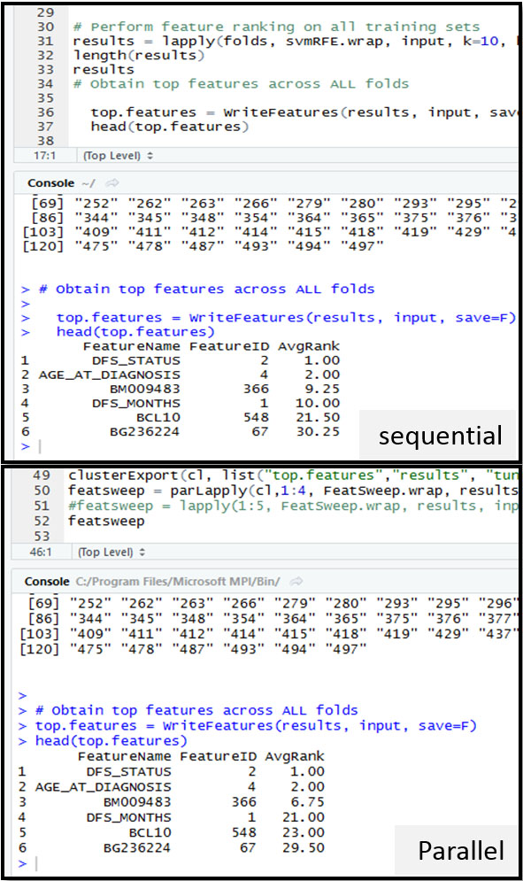
Parallel runtime relative to the sequential mode can eventually reduce by the number of processors, which is ideal because runtime depends on other things, such as data communication between processes. In all sequential implementations, we set the number of subsamples ( $k$ -folds variable) to four because, in parallel mode, only four processes can be executing simultaneously.

In Fig. 3 the results obtained by executing parallelized mSVM-RFE are compared with sequential methods. The vertical axis represents the number of samples and the horizontal axis shows execution time. It can be observed from Fig. 3 that the execution time of parallel algorithms has been a significant reduction and reports a 60 percent reduction. In this proposed parallel algorithm, some parts of the algorithm have not been parallelized. When the number of features is bigger than 100, the features will be cut in half each round. This part of the algorithm takes much time and executes sequentially. For this reason, we have not more reduction.

Figure 3.

The execution time of parallel vs Sequential mSVM-RFE.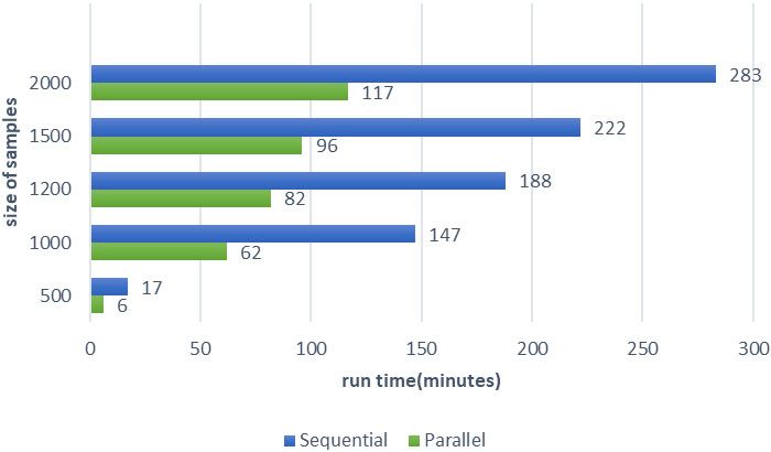

Figure 4.

The execution time of parallel mSVM-RFE with different subsamples.

In the next experiment, the number of samples was identical. First, we tested for 4 subsamples and then 8 subsamples. In this comparison, the sample size is 500 and the number of features is 600. In addition, in this evaluation, we do not consider the execution time for the generalization error.

Figure 4 shows the execution of the algorithm in a situation where the number of subsamples is 4 and 8. As we can see, in the case of 4 processors, the best runtime is achieved because each processor has only one dedicated subsample and thus more parallelism. When each processor has more than one subsamples, each processor begins to reduce features down to less than 100, which is time-consuming. In addition, each processor must run more machines due to having more subsamples. By comparing the runtime in single-core with four-cores, we find that the speed of algorithm has more than doubled. Although with 4-cores, we expect the runtime to be nearly four times higher, when the number of subsamples exceeds the number of processors, we cannot assign subsamples to the processors at one stage. Therefore, if we have 8 subsamples and 2 processors, we need to assign subsamples to processors in 4 steps, which is time-consuming. Besides, when the processors finish, the value of the features must be collected from different processors and then integrated into the master processor.

As shown in Fig. 4, with the increase in the number of subsamples, the run-time is significantly increased. However, we should not forget that the reason for creating more subsamples is actually increasing the accuracy of the algorithm. As the graphs show, when the number of subsamples is equal to the number of processors, the best balance is achieved.

Figure 5.

The classification error (Cross-Validation).

Figure 6.

The speed up.

As it was stated before, the algorithm estimates classification error for each fold in the external 10-fold. Classification error can eventually indicate which error is less fault and more suitable for classification. In addition, by comparing the classification error in parallel mode with sequential mode, we can show how the accuracy of the algorithm has changed. This error has been evaluated for data with a sample size of 500 and 600 attributes. As seen in Fig. 5, in both mSVM-RFE and parallel mSVM-RFE the minimal classification error can be reached when we use two features. It is observed that the classification error in two sequential and parallel modes is much closed. It means that parallelism has not reduced the accuracy of the algorithm.

4. Conclusion and future work

Figure 6 shows the rate of speeding up resulting from parallelism. This experiment is run on two computers running 2 and 4 simultaneous processing and in all cases, the number of subsamples is also 4. The speedup of 4 processes into one process is better than the two processes to one process. In the case of 4-cores, only one sample is assigned to each processor, but in 2-cores, each processor has two subsamples. Therefore, as the number of processors increases, we observe more speed. On a computer with 4 processors, the rate of acceleration is about two and a half. The best rate of acceleration occurred at 500 data size, which in quad-processor was about 2.8 times. In addition, in dual-processor it is about 1.90. It can be said that in this case, the best data distribution has been done, which has been proportional to the number of processors and sub-samples as well as the volume of sub-samples. We did not parallelized a small percentage of the algorithm (classification error), which is the reason for the difference between the obtained rate and the ideal state.

In addition to the parallelized part of algorithm, the classification error can also be estimated in parallel. This error is calculated for each sub-sample for the final properties. Therefore, the error calculation for each sub-instance can be done in parallel so that each processor can calculate the error for each sub-instance.

In this implemented algorithm, the support vector machine has a linear kernel that does not support non-numeric data, therefore for a wider use of the algorithm, its kernel can be changed to support non-numeric data as well. In addition, we mentioned that the algorithm for each sub-sample starts to decrease the number of features from the beginning, that is, for example, if we have 8 sub-samples and the number of features is 500, the algorithm starts reducing the number of features 8 times from 500 to 100 or less because each reduction is based on a different sub-pattern. This process can be summed up as doing it once at the beginning of the algorithm, although it may affect the algorithm’s accuracy a bit.

References

Siegel

Miller

Fuchs

Jemal

. Cancer Statistics. CA Cancer J Clin. 2021; 71: 7-33.

Rice

Wang

. Cancer bioinformatics: A new approach to systems clinical medicine. BMC Bioinformatics. 2012; 2(1): p. 71.

Moses

Nass

. Cancer biomarkers: the promises and challenges of improving detection and treatment. National Academies Press. 2007.

Joshi

Kaur

. Biomarkers in cancer. Biology, Medicine. 2016.

Panagoulias

Sotiropoulos

Tsihrintzis

. Nutritional biomarkers and machine learning for personalized nutrition applications and health optimization. 12th International Conference on Information, Intelligence, Systems and Applications (IISA 2021). Chania, Crete, Greece. 2021.

Liu

Motoda

. Computational methods of feature selection. Chapman & Hall Crc, ISBN978-1-58488-878-9, 2007.

Quo

Kaddi

Phan

, et al. Reverse engineering biomolecular systems using omic data: challenges, progress and opportunities. Briefings Bioinform. 2012; 13(4): 430-445.

Saeys

Inza

Larranaga

. A review of feature selection techniques in bioinformatics. Bioinformatics, 2007; 23(19): 2507-2167.

. Stable feature selection for biomarker discovery. Computational Biology and Chemistry. 2010; 34(4): 215-225.

10.

Guyon

Gunn

Masoud Nikravesh

Zadeh

. Feature Extraction: Foundations and Applications. Studies in Fuzziness and Soft Computing. Springer-Verlag New York, Inc. Secaucus, NJ. 2006.

11.

Devi Arockia Vanitha

Devaraj

Venkatesulu

. Gene expression data classification using support vector machine and mutual information-based gene selection. Procedia Computer Science. 2015; 47: 13-21.

12.

. A Comprehensive Comparison of Neural Network-Based Feature Selection Methods in Biological Omics Datasets. In 4th International Conference on Signal Processing and Machine Learning (SPML 2021). Beijing, China. ACM, New York, NY, USA. 2021.

13.

Panagoulias

Sotiropoulos

Tsihrintzis

. Biomarker-based deep learning for personalized nutrition. Proceedings of the 33rd IEEE International Conference on Tools with Artificial Intelligence (IEEE-ICTAI-2021). 2021.

14.

Zhou

Porwal

Zhang

Ngo

Nguyen

Ré

Govindaraju

. Parallel feature selection inspired by group testing. Proceedings of the 27th International Conference on Neural Information Processing Systems. Montreal, Canada. 2014, pp. 3554-3562.

15.

Tomczak

Czerwińska

Wiznerowicz

. The Cancer Genome Atlas (TCGA): an immeasurable source of knowledge. Contemp Oncol (Pozn). 2015.

16.

Cao

Zhang

Wang

Yang

. A fast gene selection method for multi-cancer classification using multiple support vector data description. Journal of Biomedical Informatics. 2015; 53: 381-389.

17.

Sanz

Valim

Vegas

et al. SVM-RFE: selection and visualization of the most relevant features through non-linear kernels. BMC Bioinformatics. 2018; 19: 432.

18.

Mathur

. Statistical Bioinformatics: with R. Academic Press, California. 2010.