
Abstract
Educational Data Mining has turned into an effective technique for revealing relationships hidden in educational data and predicting students’ learning outcomes. One can analyze data extracted from the students’ activity, educational and social behavior, and academic background. The outcomes which are produced are, the following: A personalized learning procedure, a feasible engagement with students’ behavior, a predictable interaction of the students with the learning processes and data. In the current work, we apply several supervised methods aiming at predicting the students’ academic performance. We prove that the use of the default parameters of learning algorithms on a voting generalization procedure of the three most accurate classifiers, can produce better results than any single tuned learning algorithm.
Keywords
Introduction
Nowadays, many universities offer innovative and high-quality education via the distance learning method. The adoption of digital technologies in education, and more general in society, establish a necessity for data and learning analytics. As the students’ needs vary, the way the distance learning courses are offered should be adapted to these needs and also to the students’ prior knowledge. In conventional education, the instructors and the auxiliary staff, guide and assist the students through the learning procedure by using different types of learning material [1, 2, 3]. In distance learning, the students schedule their study time by themselves and the successful completion of each course depends on the students’ effort but also on additional parameters, like their educational background, the psychological support of their family, and their job obligations. Many institutions that apply the distance learning methodology, include in their teaching procedure some contact sessions that are non-obligatory face-to-face contacts with lecturers and other students where questions are asked and clarification on issues are given [4].
The performance prediction is a useful information, especially when it concerns those students who fail in their quizzes and their final exams, as the instructors can intervene during the academic year and alter the applied educational methodology, based on these students’ learning style.
The prediction of the students’ performance is a hot issue in the field of machine learning. Educational Data Mining is a viable solution in this domain. The goal is the analysis of the students’ learning behavior and as well the prediction of their performance. The educational issues can be enhanced with machine learning methodologies [5]. The supervised classification methods consist of a viable aspect for this field.
In the work of [6], the authors use Pivot Tables of Excel to visualize the learners’ participation in a blended learning course. The proposed methodology is useful to discover data that affect the prediction of learners’ performance and the optimization of the course organization. Thus, a tutor is efficient to advise the students during the learning procedure. A study of the opportunity that the Learning Management Systems provide to a data scientist to record the students’ learning activity is suggested by the authors in [7]. This potential offers a benefit to students, faculty, and administration to improve important issues such as the learning procedure, the course design and the educational methodology. This cited work aims to analyze learners’ behavior and performance so that to reveal abilities useful to enhance the functionality of a distance learning course. In this study, we extend the above methodologies by using data mining and artificial intelligence in order to predict the students’ performance.
Research questions
1
2
The rest of the paper is structured as follows: Section 3 presents recent works regarding the application of classification methods in education. A detailed description of the dataset and the attributes which are used in this study are presented in Section 4. We define the algorithms in section 5. We present our experiments and our results in Section 6. The significance of each parameter in the proposed methodology, is presented in Section 7. In the same section, the methodology for predicting the students’ grades in their final exams, is also presented. Finally, in Section 8, we communicate our conclusions and we present our future research focus.
Related work
A decision tree classifier is built in [8] for detecting students at risk of failing, in an early undergraduate computer programming course. The authors use several data related to students’ assessment marks, their activity in an automatic marking system and their participation in discussion forums, in order to early identify the low performers. By using only the assessment attributes, the authors achieve an accuracy of 83%, while by using all attributes they reach an accuracy of 87%.
The authors in [9] investigate the effectiveness of familiar supervised techniques (Naïve Bayes, SVM, J48 decision tree, and multilayer neural networks) for the early prediction of at-risk students. As a risk, the study considers the eventual failure in two introductory programming courses in a Brazilian university. The first dataset is referred to 262 students attending a 10 weeks distance course and the second one is referred to 161 students attending a 16 weeks on-campus course. Both datasets contain several demographic, social, and university attributes. The experimental results show that EDM methods are effective in the early identification of low performers. Moreover, the effectiveness is enhanced after data preprocessing and fine-tuning of algorithms.
A behavioral analysis of the students and the effect of this analysis on their performance are suggested in [10]. The authors utilize the data which are derived from smartcards. The metric for the performance estimation contains the grade of each course. The poor performers are those who are at risk. The methods which are used to predict the performance are Decision Tree, Random Forest, Ridge Regression, and other algorithms. In order to speculate students’ similarity, the authors consider the presence of students in the same place (library, dormitories, teaching buildings, etc.) within a short time interval (one minute). Sleep pattern is also taken into account as students who wake up later perform worse. Moreover, the authors study the effect in different majors and during different semesters.
A study for various contingency tables is presented in [11]. The authors use these tables to predict the students’ performance. Specifically, during the semester, the performance in online exercises is considered in order to predict the students’ performance on paper-based exams, at the end of the semester. It is highlighted that the number of a student’s attempts to answer the online exercises, is associated with the grades in the final exams.
The use of the application of machine learning techniques in education is demonstrated in [12]. A case study with the prediction of the students’ grades is analyzed by the authors. Furthermore, there is use of demographical data and grades in the written assignments in order to predict students’ performance with a regression method. In addition, the authors provide a novel software tool appropriate for tutors.
In a recent study [13] machine learning methodologies such as Artificial Neural Network, K-Nearest Neighbor, K-Means Clustering, Naïve Bayes, Support Vector Machine, Logistic Regression, and Decision Tree, are presented. It is the authors’ choice to implement in Weka the prediction of the at-risk students. This prediction takes place before the students start their new academic program, i.e., pre-start data. It is highlighted that the Auto-Weka tool [14] performs the selection of the algorithm automatically with better accuracy.
An overview of studies on the prediction of the students’ performance is highlighted in [15]. Some researchers use cumulative grade point average (CGPA) and internal assessment, as data sets. The most common approaches for this prediction are the Decision Trees and the Neural Networks.
According to [16], we are able to predict the students’ failure in distance learning by using the most common classification algorithms. The authors suggest the development of a framework, which can transfer, manage and implement Machine Learning to tackle the imbalance problem in the final examinations.
A drawback of binary decision trees is confronted in [17]. It is strongly considered that the sharing of datasets from various organizations incurs this drawback. The goal is to preserve the privacy of those sensitive patterns. Furthermore, the authors compare their proposed methodology with other methodologies such as output perturbation or cryptography methodologies. The results lead the authors to conclude that the proposed method is better. In addition, with this proposed methodology the decision tree rules, which have the minimum impact than the other rules, are hidden.
Moreover, in [18] it is suggested by the authors that the privacy-preserving record linkage is confronted with private blocking techniques. The proposed technique is based on sorted nearest neighborhood clustering and it is twice faster than other existed private blocking methodologies. We also use in our experiments decision trees and k-Nearest Neighborhood algorithms.
Data coming from the learning management system Moodle are used in [19]. In addition, data have been collected from questionnaires. The goal of this cited work is to predict the students’ success or failure to pass the lesson. For this purpose, the authors use four different methods (visualization of the variables determined by the questionnaires, C4.5 decision tree, class association rules, and k-means implementation). The R language and the Weka tool are used for the implementation of the proposed methodologies.
Moreover, in [20] it is suggested by the authors the combination of classification algorithms in order to enhance the prediction accuracy of students’ performance. For the combination, the authors use the voting methodology. The algorithms Naive Bayes, the 1-NN, and the WINNOW are used.
In [21] multimodal techniques are employed for the analysis of the learning activities in a laboratory classroom. Video technology is utilized for this aim. The techniques offer great research possibilities for the investigation of various classroom and pedagogical conditions. These possibilities are appropriate for the optimization of classroom teaching and learning. The data come from audio and video recordings.
In [22] a student model for a web-based course with a subject the programming language C is proposed. The system in which this student model is incorporated attempts to identify the needs, background, and prior knowledge of the learners. This is feasible before the interaction among the system and the student so that a better experience to be available. Data analysis is used for the creation of the model. The collection of the data comes from an initial implementation of the system with the name ELaC.
Many aspects of Learning Analytics (LA) are covered in the chapters of [23]. Specifically, subjects such as LA in distance learning in postsecondary education, prediction of students’ performance in a blended introductory course, prediction of dropout students, dashboards for project and problem-based learning are negotiated in the [23] book.
Some well-known algorithms are used [24] in order to remove noisy and redundant data from the data set used in predictive data mining. It is highlighted that this methodology is efficient to enable knowledge discovery as an easier task.
Dataset parameters used in the study
Dataset parameters used in the study
In this study, we used a dataset provided by the Hellenic Open University (HOU), an institution which is mastering the open and distance learning education and always seek modern and innovative ways of communicating Knowledge [25, 26, 27]. Our study focused on the year-long class module called “Algorithms and Complexity”, a module on the subject of algorithms introduction of the Informatics graduate programme. It is the authors’ preference to characterize each instance by the values of 10 variables (Table 1). These instances consist of five submitted projects and five not obligatory attended consulting Sessions (aka contact session (CS)).
The completion of the module requires the submission of five projects and a grade equal to or higher than five, in the final exams. Students can undertake the final exams of the module, only if they have successfully completed the four or five projects with a total score of twenty-five or more, on a ten-grade scale for each project. During the academic year, students have the opportunity to attend, if they wish, five attended consulting sessions of four-hours each.
In the figures: Figs 1 to 10, we illustrate our dataset. In each pair of figures, we can make the following observations. The orange bar of Figs 1, 3, 5, 7, and 9, regards the percentage of students over the total number of students who have attended each attended consulting session, while the blue bar corresponds to the percentage of the students over the total who have not attended each consulting session. All figures regard the students who have passed the course. The orange bar in Figs 2, 4, 6, 8, and 10, denotes the range of the grades in the corresponding submitted project for those who have passed the final exams. The blue bar denotes the range of the grades of the same project for those students who have failed in the final exams. The vertical line of each interval denotes the mean grade of the grades’ range.
In Fig. 1, we observe that the majority of the successful students have attended the first consulting session.
Percentage of the successful students who have attended or not the contact session 1.
Grades range of students who pass or fail the submitted project1.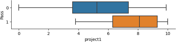
Percentage of the successful students who have attended or not the contact session 2.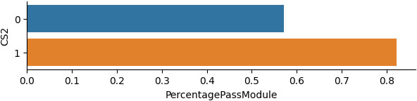
Grades range of students who pass or fail the submitted project2.
Percentage of the successful students who have attended or not the contact session 3.
Grades range of students who pass or fail the submitted project3.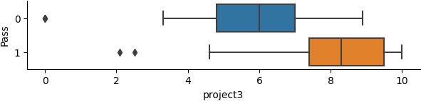
Percentage of the successful students who have attended or not the contact session 4.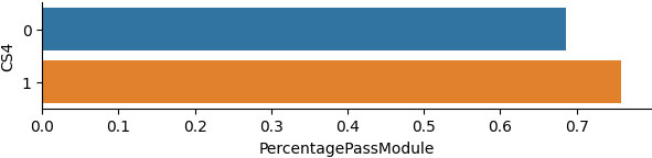
Grades range of students who pass or fail the submitted project4.
Percentage of the successful students who have attended or not the contact session 5.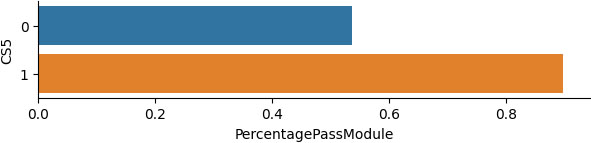
Grades range of students who pass or fail the submitted project5.
Based on Fig. 2 it is apparent that the successful students who attended the first contact session have higher grades in the first submitted project than their fellow students who did not attend this particular session.
According to Fig. 3 it is obvious that many successful students attended the second contact session. The percentage of the students who passed the exams but they didn’t attend the second contact session over the total number of students who didn’t attend the second session is low. Thus, a small number of students are not influenced positively from the attendance of the second consulting session.
In addition, as we observe in Fig. 4 all the successful students who attended the second session obtained higher grades than those who did not participate in it.
Similar observations can be made for those students who did and did not participate in the third contact session, as presented in Figs 5 and 6.
Figure 7 demonstrates that the successful students who attended the fourth contact session are almost equal to the successful students who did not.
As it is apparent in Fig. 8, the students’ grades, after participating in the fourth consulting session, are higher than the grades of those students who did not participate in it. The difference among the mean grades is not negligible.
According to Fig. 9 the percentage of the successful students who attended the final consulting session is higher than the percentage of the successful students who did not. The successful students who attended the contact sessions 1 and 2, 3 and 5 are more than those who attended the contact session 4.
As a conclusion of the Table 2, we observe that most students have attended the first two Contact Sessions (CS). Furthermore, the students who attended the CS2 are slightly less than the students who attended the CS1.
Combination of contact sessions participation and relevant statistics
Grade value limit of project1 to project4 and the corresponding percentage of the successful students
Participation of the students in each Contact Session and the corresponding mean project grade and percentage of passed students
Grades distribution of each submitted project.
The students’ grades after attending the fifth contact session, are better than those of the students who were absent in this session, as we can observe in Fig. 10. It also should be noted that many students have a fail grade in the submitted project5 and all of them were absent in the corresponding contact session. This regards almost the half of the successful students. That happens, due to the difficulty of the final project. It is also a proof that the half successful students made an effort to study the submitted projects themselves without the help of a third person.
In Figs 2, 4 and 8 it is obvious that there is a small overlap between the grades of those students who attended the first, second and the fourth contact session, in comparison with the grades of the students who did not participate in these sessions. Figure 10 presents that this overlap is bigger for the fifth session which is the final session. This can be attributed to the fact that there were many students in this class who prefer only the remote communication with their tutor and their fellow students. Alternatively, there is a chance that those students assign their projects to third persons and as a result they had no questions to pose.
By using and combining classification algorithms with this dataset, we are able to predict the students’ performance. Moreover, we can locate the more informative attributes for the prediction. In the following sections, we present a methodology with this goal.
Initially, we describe the algorithms with which we experiment. Furthermore, we compare the combinations in pairs of contact sessions. Each combination is represented by a binary number with two digits. When a digit is 1 this denotes the present students in the corresponding contact session. Useful conclusions for each pair are the mean and the median grade in the final exams, the percentage of the successful students and also the numerical value of those students (Table 2).
The grades of each project and the percentage of the successful students who achieve a grade greater or smaller than a value are given in the Table 3. For example the 86.2069% of the successful students achieve a grade greater than 6.5 in project3. The 75% achieves a grade greater than 3.5 in project1, the 73.9726% achieves a grade greater than 5 in project2 and the 81.3559% achieve a grade greater than 5 in project4.
In Table 4, we observe the percentage of the students who passed the final exams and also they had participated in each Contact Session or not. In addition, we observe the mean grade and the median grade of each submitted project and the number of the successful students according to their presence or absence in each Contact Session. The median grade separates the numerical value of the higher half of a sample, a population or a probability distribution from the lower half.
In the Fig. 11 we can observe the grades distribution of each submitted project according to the participation or not to each corresponding Contact Session.
A decision tree is a classification method which uses for representation purpose, a collection of decision nodes connected by branches. Each decision node consists of the tested attributes whereas the outcome produced is a branch. The goal is to classify the instances according to the attributes they contain. In our approach, we use the CART decision tree [28]. It is a binary tree which produces two branches for each decision node. CART uses the Gini Impurity function [29] to measure the attribute selection in order to build a decision tree. This function determines the calculation of the sum of squared probabilities of each class. After the training, the algorithm selects as a root node the attribute with the highest information calculated by the Gini Index. Similarly, the maximum Gini coefficient is selected in every split. When there are not remaining decision nodes, the complete tree is grown.
Naïve Bayes is an algorithm that assumes that the dependency relationships, which a classifier uses among the features, are unknown [29]. The simplest assumption is taken into account i.e. when a category is given, the features are conditionally independent. The conditional probability assumes that the features are conditionally independent by considering the product of features’ conditional probabilities.
The k-Nearest Neighbor is an algorithm that applies instance-based learning [30]. Initially, the algorithm trains some data in order to find a classification for a new unclassified entry. To achieve this, a comparison is performed to the most similar entries in the training set. The algorithm takes into account the nearest points of each centroid in each neighborhood to perform classification. In case some random points are inserted after the training, the classification approximates the initial clusters which accrue after the training. These random points are also called noise. In case one removes a data point from the classification of kNN and executes the algorithm to predict a class for this point, then the incorrect prediction is called a cross-validation error. It is the authors’ preference to use 3NN in the experiments.
Logistic regression is a methodology domain that is useful for the description of the relationship between a categorical response variable and a set of predictor variables. It can be used for binary or dichotomous variables, or in variables with more than two categories [31]. The latter case is called polychotomous logistic regression. In order to interpret the outcomes of the above methodologies, the term of the odds ratio should be used. The data are processed in the terms of logit functions and maximum likelihood estimation.
The neural networks have a structure of three layers. The first layer is called the input layer, the intermediate layers are called hidden layers and the last layer is called the output layer. The training of the neural networks detects the optimal weights in order to achieve the maximal accuracy for new data inputs. This is feasible by iterating through training aiming to improve the accuracy. At the end of the training, the model is efficient to estimate the output for a new data pattern. Multi-Layer Perceptron (MLP) is a Feed-Forward NN and it consists of one hidden layer. The Feed Forward NN allows the signal to propagate in one direction only, from input to output. In the work of [32], the authors use the Moth-flame Optimization to find the optimal weights of MLP by minimizing the Mean Squared Error of actual and desired outputs and to obtain a high classification rate.
The goal of using an SVM is to find the separating hyperplane which has the largest margin. The separation among two classes is determined as margin. The classifier is generalized better according to the size of the margin. More specifically, the hyperplane is selected so that the distance of every data point from each side of the hyperplane, is maximum. In this case, the corresponding linear classifier is called the maximum margin classifier. The linear classifier SVM is useful to classify the most difficult patterns because of the optimal hyperplane separation property [33, 34].
The Random Forest [35] is a classification algorithm that considers a large number of different decision trees. The prediction is the one that corresponds to the decision tree with the most votes. The procedure of selecting a random sample from the dataset with a replacement for individual decision trees is called bagging. The bagging and the random features are used in order to create a forest of decision trees that have a more accurate prediction, in comparison with each individual tree.
The boosting term corresponds to a method that enables a more accurate prediction rule. This results from the combination of rough and moderately inaccurate rules of thumb. The most popular algorithm is the AdaBoost [36] where each example is weighted. Initially, all the examples are assigned with the same weight. In order to classify the examples, the algorithm considers the distribution of the weights. The boosting algorithms use a weak learner. A prediction is binary (correct or not). According to the verification or not of a correct prediction, the algorithm adapts the weight of each example. In order to achieve the final classification, the algorithm uses the weights which the weak learners determine.
According to [37] there is the ability to combine classification algorithms. Each classifier votes for each decision. The class, which the authors prefer to select, comes from the combination of the algorithms with the larger number of votes. This selection is also called a consensus decision.
Machine learning algorithms.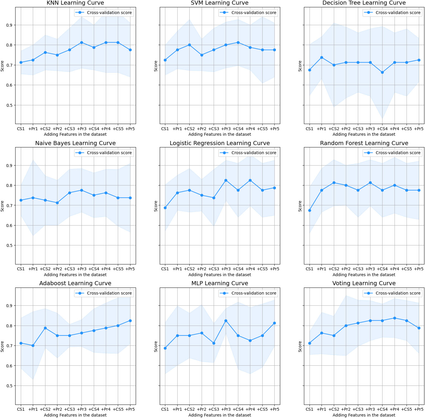
Random forest feature importance.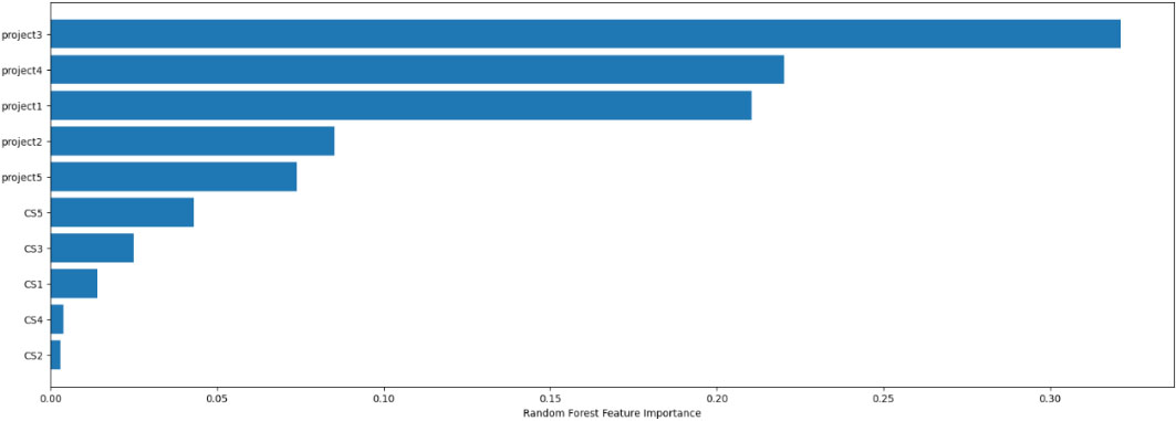
Permutation importance.
Mean shapley values.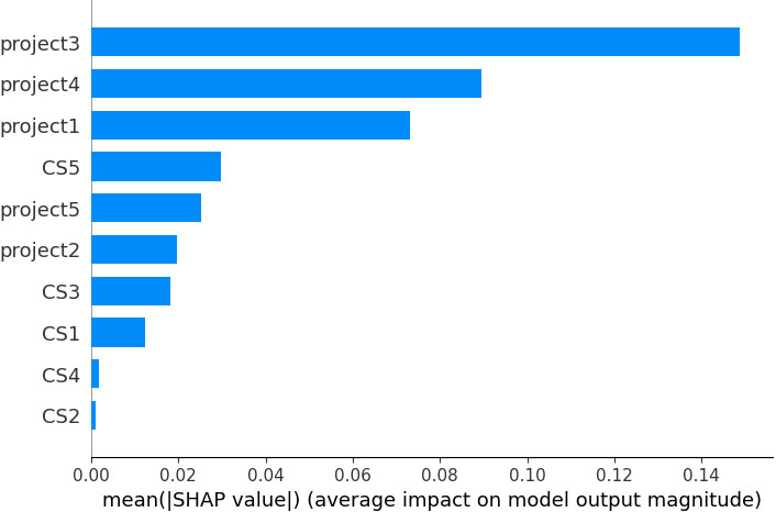
We carry out the experiments by using the Scikit-learn, and we conduct them in ten successive steps. Initially, we separate the data into groups of the same size. The total number of groups is 10. The 1
In every iteration, each group is considered as test data and the remaining groups are the training data set. Therefore, for each group, it is the authors’ preference to calculate the accuracy of each classifier algorithm applied to the training of the remaining groups. The current group is considered as a test data set. We obtain the accuracy of each algorithm for this procedure with the cross-validation estimation.
Hyperparameters are the parameters that the machine learning algorithms use to control the training procedure. These parameters determine the degree to which the model obtains the desired output during training. The correct combination of hyperparameters that we use is the one that contributes to the estimation of a maximum or the minimum value of a function. In order to calculate this combination, a random search of the hyperparameters in a grid of those parameters is employed. The performance is computed by cross-validation. This method is applied to the following machine learning algorithms in Fig. 12.
The default parameters of the three most accurate classifiers on a voting generalization procedure can produce better results than any single tuned learning algorithm.
Feature importance
In Fig. 13, the significance of each parameter is highlighted in order to make a prediction, in comparison with the significance of the other parameters. We assign to our data the most relevant or most irrelevant parameters to calculate the target variable with each predictive model. Moreover, it is the authors’ preference to use the Random Forest algorithm [35] for parameter importance implemented in scikit-learn [38]. There is a description of this algorithm in the previous Section 5.
Using Feature Importance, we can identify the features of a model which are most or least significant in order to perform a prediction. Initially, we apply a model to our data even if this model does not support native feature importance scores. Then, we perform predictions for each feature even though the values of each feature (column) are shuffled. This procedure is repeated for a small number of times (up to 10 times). The mean score for the importance of each feature, and the distribution of those scores in each iteration, are determined. With the application of this method, we are able to identify the feature importance metric which affects the performance. This metric can be the mean squared error for regression and accuracy for classification. The Feature Importance of the Random Forest algorithm is illustrated in Fig. 13, while the Permutation Feature Importance by shuffling the features is presented in Fig. 14.
With the use of the methodology proposed in [39], we are able to measure the importance of each feature of various prediction methods. This is necessary to make these methods easy to comprehend. Game theory is used to find a unique solution. Next, we compare the predictions by including or not each feature. In addition, we consider three properties for reasons of approximation. These properties are local accuracy, absence, and consistency. Specifically, we calculate the Shapley values from game theory by employing a weighted linear regression as it is illustrated in Fig. 15. Linear regression and Shapley values are combined in the above-cited work. The authors of [39] consider the mean as the best least-squares point estimation for a set of given data elements. The computational efficiency of this method offers a more accurate estimation with fewer computations of the original model in comparison with other estimations based on samples.
The results lead us to conclude that the most informative attributes according to all examined feature importance strategies are Project3, Project4, and Project1 grades.
Final grade estimation
In this subsection, we build a linear regression model for predicting the final grade in Eq. (1).
Grade
In order to run this regression, we separate the data into 10 subsets. We reserve one subset to test the model while we use the other subsets to train the model. As a next step, we repeat the regression for each subset used as a test set. It is the authors’ preference to trace the prediction error and to calculate the average of the 10 traced errors. This performance metric is called the cross-validation error. The algorithm is called Repeated K-fold cross-validation. We run a 10 cross-validation and we calculate the mean values for mean absolute error and root mean squared error. Furthermore, we use the Root Mean Squared error to calculate the average difference between the observed and the predicted values which the model produces. The Mean Absolute Error is a metric that we use instead of RMSE as it is less vulnerable to outliers.
Mean Absolute Error: 1.7958424729267497 Root Mean Squared Error: 2.2347550840313413
Discussion and concluding remarks
In this study, we investigate the effectiveness of active learning algorithms to predict students’ performance (pass or fail) in a distance learning undergraduate course module in the HOU. The prediction focuses on the grades achieved in the students’ final exams. The prediction of the students’ performance has been an interesting and highly important research topic for educational institutions in the recent years. Identifying as soon as possible, the low performers in a class, could lead to the development of personalized learning strategies for enhancing the learning outcomes, in accordance with the learning profile.
In order to approach this matter with artificial intelligence techniques, we combine several machine learning algorithms to predict the students’ performance. The most significant factors for the prediction are their grades in Project3, Project4, and Project1. The performance of each algorithm is calculated with cross-validation. We calculate the mean score for the importance of each feature. Then we calculate the distribution of the mean scores in each iteration of the Feature Importance method. Hence, we are capable to identify the feature importance metric which affects the algorithm performance. Furthermore, we can find a unique solution by employing Game Theory and Shapley values applied to a weighted linear regression. The average difference between the observed and the predicted values of the model are measured with the Root Mean Squared error or with the Mean Absolute Error.
We employ a generalized procedure based on votes. By using the classification algorithms which correspond to the three best accurate estimations we prove that they perform better than any single balanced learning algorithm.
There is a clear need for further insights into ascertaining the salient features that contribute to both a highly predictive and explanatory model. In future work, we will explore these features. Moreover, as a test benchmark, we will use data mining techniques to explore the students’ socialization during the contact sessions with associations among variables. In addition, we will cluster the students with similar performance and presence in the Contact Sessions with fuzzy classification. The sequences of presence in Contact Sessions and grades achieved in the submitted projects will be explored with hidden Markov models.