An effectual recommendation model using hybrid learning models for early detection of Alzheimer’s disease

Abstract

Alzheimer’s disease (AD) is a neurodegenerative disorder that affects millions of individuals worldwide, causing progressive cognitive decline. Early prediction and diagnosis the AD accurately is crucial for effective intervention and treatment. In this study, we propose a comprehensive framework for AD prediction using various techniques, including preprocessing and denoising with Multilayer Perceptron (MLP) and Ant Colony Optimization (ACO), segmentation using U-Net, and classification with Spatial Pyramid Pooling Network (SPPNet). Furthermore, we employ Convolutional Neural Network (CNN) with SPPNet for training and develop a chatbot for recommendation based on MRI data input. The preprocessing and denoising techniques play a vital role in enhancing the quality of the input data. MLP is utilized for preprocessing, where it effectively handles feature extraction and noise reduction. ACO is employed for denoising, optimizing the data to improve the signal-to-noise ratio, and enhancing the overall performance of subsequent stages. For accurate segmentation of brain regions, we employ the U-Net architecture, which has shown remarkable success in medical image segmentation tasks. U-Net effectively identifies the regions of interest, aiding in subsequent classification stages. The classification phase utilizes SPPNet, a deep learning model known for its ability to capture spatial information at multiple scales. SPPNet extracts features from segmented brain regions, enabling robust classification of AD and non-AD cases. To enhance the training process, we employ CNN with SPPNet, leveraging the power of convolutional layers to capture intricate patterns and improve predictive accuracy. The CNN-SPPNet model is trained on a large dataset of MRI scans, enabling it to learn complex representations and make accurate predictions. Hence the proposed work can be integrated with a chatbot that takes MRI data as input and provides recommendations based on the predicted AD probability. Experimental evaluation shows that the combination of preprocessing, denoising, segmentation, and classification offers a comprehensive solution for accurate and efficient AD diagnosis and management.

Keywords

Alzheimer’s disease early detection learning algorithms recommendation model neurodegenerative disorder and MRI-based diagnosis

1. Introduction

Alzheimer’s disease (AD) is a leading cause of disease in brain. It is caused by a problem called intellectual disability, which leads to a decline in intellectual abilities, alterations in actions, and memory decay. AD impacts the flexibility required to be developed [1]. Although medical science has advanced, there is still no active treatment for Alzheimer’s disease (AD). Instead, the best approach is to delay the disease’s development [2]. In order to stop Alzheimer’s from progressing to more severe stages, it is crucial to recognize the signs of the disease as soon as possible in the beginning stages [3]. The most prevalent type of AD is cognitive impairment, which is a result of the disease’s absence of a curative therapy [4].

AD advances gradually before clinical indicators become apparent. There are alterations in the cerebral fluid, like a 50% reduction in AB42 because of more p-Tau and amyloidosis building up in the brain. As a result, both kinds of tau are increasing, reflecting the damage to neurons that leads to dementia and ADs. The assessment of the depletion of protective capacities that lead to ADs is made by APOE 4 alterations, which have toxic consequences. People with Alzheimer’s rise every five years, based to the CDC. In 2050, there are expected to be 152 million people living with the illness, according to the WHOs. AD’s beginnings are still unknown [5]. However, some hypotheses propose that neurons in the brain develop higher phosphorylated molecules of proteins and amyloid plaques [6]. As a result, the accumulation of tangled neurofibrillary fibers or plaques made of amyloid causes neurons to undergo destruction [7]. MCI is the beginning phase of AD [8]. People who are at this stage may still do everyday tasks but have modest impairments in their cognitive capacity. 20% of those over 65% have MCI, and 35% of them develop AD within three to five years [9]. So, depending on how soon it is discovered, MCI either stays stable or progresses to AD. Dynamic patterns [10] that manifest early, before AD develops, describe structural as well as functional alterations in AD. With the use of MRI imaging, changes in patterns can be recorded, brain shrinkage can be measured, and degeneration may be recognized [11]. Functional MRI also monitors changes in brain activity, blood flow, and connections [12]. GABAs, GSHs & NAAs receptor alterations are detected using MR spectroscopy. Pictures alone cannot provide information about an MRI, hence image reconstruction is necessary to turn the received raw data into pictures that a physician can understand [13].

The information processing on current MRI appliances translates info into pictures [14]. The inner workings and functions of the brain are extensively studied using brain scanning methods. So, MRI helped doctors look at functionally busy parts of the cognitive system to find Alzheimer’s disease earlier [15]. MRI feature retrieval manually requires knowledge, skill, and work. Thus, AI diagnosis is needed to address these issues. To identify MCI phases, precise data is required. Deep learning models can therefore successfully extract the characteristics of each AD step. This work focuses on constructing systems that can detect AD in its early stages utilizing fused characteristics, extracting characteristics using deep learning algorithms, and combining characteristics from a variety of deep learning algorithm, as well as integrating deep learning characteristics with organic characteristics.

The biochemical and medical characteristics of the various phases of Alzheimer’s illness are similar, making it difficult to differentiate among them. CNN’s characteristic extraction and classifying do not provide results that are accurate enough to differentiate among Alzheimer’s phases. In addition, there persists an absence of precision in the extraction and classification of the organic characteristics. Thus, by integrating CNN and handmade traits, our research helped separate Alzheimer’s phases and forecast them efficiently.

The proposed works’ novel contributions can be summarized in three points:

•
Integration of advanced techniques is to enhance the accuracy of AD prediction. The use of U-Net architecture enables accurate segmentation of brain regions, aiding in subsequent classification stages. Additionally, the incorporation of SPPNet captures spatial information at multiple scales, improving the robustness of AD and non-AD classification. The integration of MLP preprocessing and ACO denoising optimizes the quality of input data, enhancing overall performance.
•
The utilization of SPPNet for classification enables the capture of spatial information at multiple scales. SPPNet effectively extracts features from segmented brain regions, contributing to robust classification of AD and non-AD cases.
•
Any bot-based applications’ can take MRI data as input and provides recommendations based on predicted AD probability is a significant contribution. The chatbot assists healthcare professionals in interpreting MRI results and making informed decisions regarding patient care.

The remaining portions of this work are structured as, a variety of earlier research towards the early recognition of Alzheimer’s illness are discussed in Section 2. Techniques and resources for assessing MRI images of Alzheimer’s illness are presented in Section 3 along with the effectiveness of data for the proposed methods to identify Alzheimer’s disease. The effectiveness of the proposed approach is discussed in Section 4. Section 5 presents overall conclusion of the proposed findings.
2. Review of previous literature

The given section describes a thorough evaluation of prior studies on a particular subject. The pertinent earlier research must be listed, described, summarized, reviewed objectively, and explained in this evaluation.

In [16] used the data collected by OASIS and enhancement of images to identify AD. They performed each trial with 98.2% accuracy using transferable learning. [17] integrated MRI with FDG-PET utilizing SVM to enhance AD detection. FDG PET and MRI pictures were accidentally erased from the ADNI and Leipzing Participants systems. They were able to achieve an accuracy rate of 87.8% for ADNI information sets. To aid in the recognition of Alzheimer’s illness, MCI and policies [18] present a Probabilistic classification algorithm. They fared far better than some well-known classifiers, such as NB, LRC, ANN, DT Adaboost-enhanced selection basis. Though fold’s Probabilistic kernelization technique in [19] provided mediocre results when identifying MCI-converter & MCI non-converter it might accurately identify among people with Alzheimer’s and healthy control subjects.

[20] Enhanced iterative trace ratio (iITR) technique excelled the PCA, locality protection projections (LLP), and selection boundaries criteria in solving the TR-LDA issue in dementia research. They utilized two datasets (PET and SPECT) encompassing both AD individuals and normal controls. The 91% effective NMF-SVM. [21] Discovered that VBMs & KNNs had a precision of 90.25%, a sensitivity of 80.25%, as well as specificity of 75.52% when evaluating MRI images for individuals both with and without MC. T. [22] Have shown the value of using already trained networks as a basis for creating supplemental networks. Two additional research models, Google Net and ResNet, are improved by Python’s Tensor framework and so come pre-trained on ImageNet, giving them a greater ability to discern among a wide range of real-world picture types. The simulations used in this investigation were limited to being educated on completely linked networks after starting out on partly interconnected network.

To confidently identify moderate dementia on MRI, it is necessary to increase data numbers. [23] Use Augmented & TL approaches. Utilizing OASIS2, the overall correctness for MCI vs. Normal Controls were 90.6%. Displacement Distortion Imaging patterns show a horizontal compactness for AD Diagnose. By converting the information from MRI information to DTI images, transfer learning, as described by [24], is possible. Prior to uploading the information to the DTI database utilizing the ADNI database repositories for Normal sample classification, AD, and MCI, they applied significant novel augmenting procedures for training the algorithm utilizing MRI [25, 26, 27, 28, 29]. Discriminated among patients who had MC & healthy consents using FreeSurfer yielding SVM, yielding an accuracy of 82.89% and a specificity of 78.90%. [30] used SVM for distinguishing among Alzheimer’s illness as well as other types of FTDs with a precision of 79.9%, a specificity of 77.9%, with sensitivity of 82.72%. [31, 32, 33, 34, 35] Table 1 presents the overall results of the section.

Table 1
Review on ADs forecasting techniques in existing researches

Ref no.	Methods	Pros. and cons.
[25]	(SVMs, with K-NNs & LDAs) Partial least squares	• Pros: Effective for both linear and non-linear classification, handles high-dimensional data well, good generalization performance. • Cons: Computationally intensive, sensitive to kernel choice and hyperparameters, requires careful preprocessing, can be affected by imbalanced datasets.
[15]	SVMs & Non-negative Matric Factor	• Pros: Non-negative representation for interpretability, handles high-dimensional data, effective for feature extraction and clustering. • Cons: Requires careful initialization and regularization, may not converge or find global minimum, limited in handling missing data, sensitive to factorization rank.
[16]	Meta Evaluation & SVMs	• Pros: Combination of SVM models for improved performance, model selection and ensemble learning, systematic evaluation, and comparison. • Cons: Additional computational resources, complexity increases with models, additional hyperparameters, challenging interpretability.
[17]	Multifold Bayesian kernel	• Pros: Combination of Bayesian learning and kernel methods, incorporation of prior knowledge, efficient handling of high-dimensional data, probabilistic outputs. • Cons: Requires appropriate prior distributions, complexity increases with dataset size, sensitivity to kernel choice, challenging interpretability.
[18]	Kernel PCAs, Trace Ratio (TR), LDAs	• Pros: Nonlinear dimensionality reduction with Kernel PCA, focus on discriminative power with TR LDAs, capture complex relationships, suitable for feature extraction. • Cons: Complexity increases with dataset size, sensitivity to kernel choice, challenging interpretability.
[19]	BNNs	• Pros.: BNNs provide a measure of uncertainty for predictions, which is useful in decision-making and risk assessment. The uncertainty estimates can help identify cases where the model is unsure or where the input data is ambiguous. • Cons.: BNNs can be computationally demanding compared to standard neural networks. Bayesian inference involves sampling from posterior distributions, which can increase the training and inference time. This complexity may restrict the scalability of BNNs to large datasets.
[20]	Methods, on K-NNs	• Pros: Simple and easy to implement, no training phase, flexible, adapts well to local patterns. • Cons: Computationally expensive for large datasets, sensitive to distance metric choice, requires optimal value of K, struggles with high-dimensional and imbalanced data.
[24]	FreeSurfer, SVMs	• Pros: FreeSurfer provides automatic brain segmentation and cortical surface reconstruction, SVMs offer effective classification. • Cons: FreeSurfer may require manual intervention for accurate results, SVMs can be computationally intensive, requires careful preprocessing.
[21] [22]	TLs TLs	• Pros: Utilizes knowledge from a source domain to improve performance in a target domain, reduces data and computation requirements, enables knowledge transfer. • Cons: Requires suitable source domain and task similarity, potential domain shift issues, performance dependent on transferability, challenges in fine-tuning.
[23] [14]	TLs, MRIs to DTIs TLs	• Pros: Transfer learning applied from MRI to DTI data, leveraging knowledge from MRI domain for DTI prediction, potential improved performance. • Cons: Domain shift challenges from MRI to DTI, requires careful selection of transferable features, potential loss of information between domains.

3. Proposed methodology

3.1 Data pre-processing

Data preprocessing plays a crucial role in improving the performance of machine learning models by transforming raw data into a suitable format. In this research paper, we propose a hybrid approach that combines the power of Multilayer Perceptron (MLP) with the optimization capabilities of Ant Colony Optimization (ACO) for data preprocessing. The objective is to leverage ACO to select the most relevant features or attribute subset, thereby enhancing the accuracy and generalization capabilities of the MLP model. We present the mathematical formulation of the proposed approach, outlining the key steps involved in the integration of ACO with MLP. Experimental results on real-world datasets demonstrate the effectiveness and efficiency of the proposed approach compared to traditional preprocessing methods.

3.1.1 Multilayer perceptron (MLP)

The MLP is a popular feedforward neural network architecture that consists of multiple layers of interconnected nodes (neurons). It is trained using backpropagation and gradient descent to learn the mapping between input and output data.

3.1.2 Ant colony optimization (ACO)

ACO is a metaheuristic algorithm inspired by the behavior of ants when searching for the shortest path. It uses pheromone deposition and evaporation to find optimal solutions in complex problem spaces. This hybrid approach combines MLP and ACO for data preprocessing. The main steps of the proposed approach are as follows.

Initialization

Initialize the ant colony with a set of features (attributes) as candidate solutions. Set the initial pheromone levels for each feature to a small positive value.

Feature evaluation

Evaluate the quality of each feature subset using an objective function, such as classification accuracy or information gain.

Update the pheromone levels of features based on their fitness values.

Feature subset selection

Perform a probabilistic feature selection process based on the pheromone levels. Use the probabilities to select a subset of features for the MLP model.

Training the MLP model

Train the MLP model using the selected feature subset as input. Update the weights and biases of the MLP using backpropagation and gradient descent.

3.1.3 Mathematical formulation

Feature Evaluation is, Let F be the set of features, and A be a subset of features. Let fitness(A) be the fitness value of subset A, evaluated using an objective function.

Pheromone Update consider $\tau{\_}ij$ represent the pheromone level between feature $i$ and feature $j$ . Let $\rho$ be the pheromone evaporation rate, and $\Delta\tau{\_}ij$ be the change in pheromone level. The pheromone update equation is given by Eq. (1):

$\displaystyle\Delta\tau\_ij=\left({1-\rho}\right)\ast\Delta\tau\_ij+\rho\ast% \Delta\tau\_0$ (1)

where $\Delta\tau$ _0 is a constant representing the pheromone deposited by successful ants.

Feature Subset Selection assumes $P{\_}ij$ be the probability of selecting feature $j$ given feature $i$ . The probability of selecting feature $j$ is given by Eq. (2):

$\displaystyle P\_ij=\left({\tau\_ij\wedge\alpha\ast\eta\_ij\wedge\beta}\right)% /\Sigma\_k\left({\tau\_ik\wedge\alpha\ast\eta\_ik\wedge\beta}\right)$ (2)

where $\alpha$ and $\beta$ are parameters that control the relative importance of pheromone levels ( $\tau)$ and heuristic information ( $\eta)$ .

Figure 1.

Overall flow of the proposed work.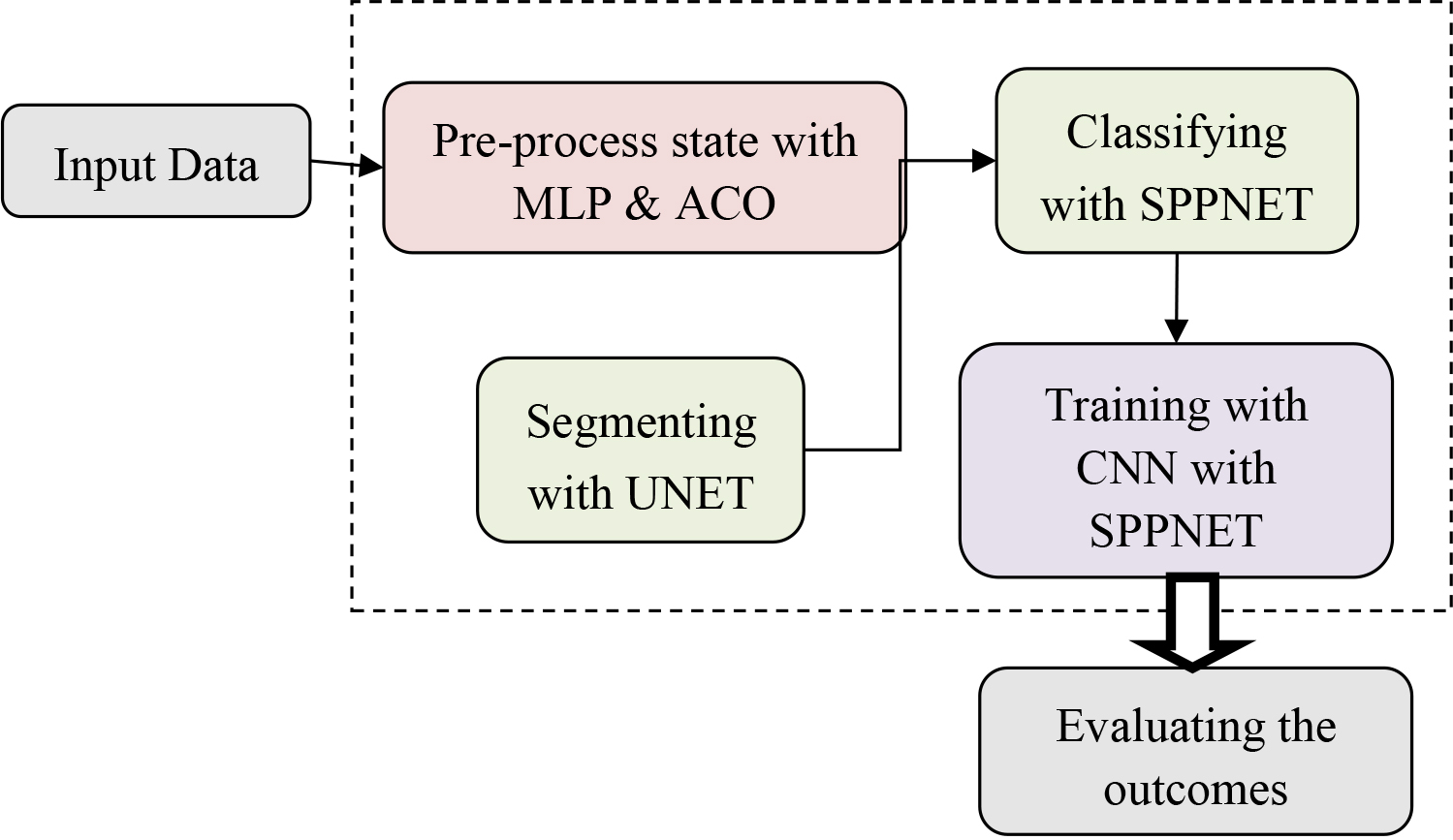

3.2 DL utilizing UNet with images information

AD has been classified using UNet using just MRI image information. The model used Keras, which is the TensorFlow. UNet is a residue machine learning system (as well as 50 levels) designed to solve the issue of elevations that disappear during CNNs back-propagation. It created the UNet model, and a collection of these UNet systems of different depths received prizes for images classification. As soon as over-fitting is taken into account, raising the network’s level could improve the precision of it. However, the issue with increasing the depth lies in the fact that the information needed to modify the number of weights that emanates via the network’s side via contrasting the actual situation with predictions (seen against forecasted), is extremely little at the network’s beginnings as a result of the increasing deep. Essentially, it shows that previous stages are still mainly forgotten. Because the amount of the gradient in the linear optimization approach that aims to change constants goes extremely close to zero, this issue is known as the “vanishing gradients” issue. The second issue with creating ever-more complex networks is that done blindly creates tiers through optimisation on a massive input field. The difficulty to learn is so increased. Residue interactions, which construct a network utilizing residual model sections, can be used to train these sophisticated networks. This problem is known as degradation. The ResNet-50 topology can be found the cross-entropy (Eq. (1)) losses assess category was selected as the best option.

The UNet model mostly consists of convolution layers. In order to identify pictures, neural systems use a variety of filtering (such as a 3 *3 pixel size filtering). Advances are made over the original picture to manipulate the filters. The learnt elements of the filters were multiply by the ranges of photos. Result of such filtering was essentially down sampled yet retaining the most relevant characteristics. UNet taxonomy is shown in Fig. 2.

Figure 2.

Illustration of IUNet for AD recognition.

3.2.1 Improved U-NETs for segmentation

It has been widely used to diagnostic picture classification, a process that integrates low-level and high-level data. This Improved U-Nets design improved on the 2D U-Nets by substituting all 2Ds processes for the 3Ds equivalents in order to better use information based on volume. Figure 1 within this piece provides an illustration of the 3D U-Net layout. It has two paths: down sampling and the upsampling Four steps have been included along the reduction procedure. Two 3 $\times$ 3 $\times$ 3 convolution layers, a BNs with a ReLUs follow every phase. Normalization in batches lowers covariance shift and prevents an overfitting by reducing hidden unit’s variables. At the conclusion of each step, a 2 $\times$ 2 $\times$ 2 maximal pooling having intervals of 2 is added for down samples. After each level, the total amount of channel features is increased. There are four steps in the up sampling route as well. An expanding layer of 2* 2* 2 kernels by stride of 2 is included in each stage, preceded by a convolutional level using BN and ReLU. Two 3 $\times$ 3 $\times$ 3 levels of convolution follow, followed by BN and ReLU. Phases in the reduction route are linked to phases with identical quality in the expanding path to reduce knowledge leakage. We use an element-wise combination as opposed to a concatenated operators for relationships, which is distinct from the conventional U-Net.

3.2.2 Recurring block of residual

It remaining the connections are used to address the problem of gradients disappearing. On a variety of tough assignments, with residual connections function well. The definition of the residual connection is given by Eq. (3),

$\displaystyle\textit{Xl}=\textit{Fl}\left({xl-1}\right)+h\left({xl-1}\right)$ (3)

When $X_{(l-1)}$ & $x_{l}$ are the lth unit’s inputs and outputs, respectively, $h(x)$ is a unique translation where $h_{(xl-1)}=x_{(l-1)}$ . These functions were denoted by $\textit{Fl}()$ corresponds to the l-th unit. Two convolutional layer structures with activation capabilities (BN & ReLU) are present in the function. The process of activation (BN plus ReLU) is carried out after removing the weight level in a simple residual blocks. The process of activating is carried out via a “preactivation” component.

Figure 3.

Structure of (a) residual for 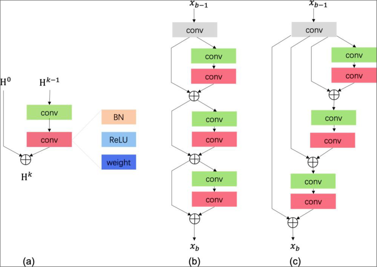$k^{th}$ unit (b) 3 residual units (c) 3 residual units with a recursive.

This work utilized a recursive leftover blocking. Figure 3(c) depicts the framework of the recurrent residual block. The recurrent remaining blocks has many remaining units. Figure 3(a) is an example of a residual unit. The residual routes aid in learning very complicated characteristics. The formulation of the remaining unit is,

$\displaystyle Hk=G\left({Hk-1}\right)=Fk\left({Hk-1}\right)+Ho$ (4)

where $k=$ 1, 2, …, $K$ , $K$ be the residuals units in a recursion remaining interfere with, and $H^{k}$ is the outcome of the $k^{th}$ remaining unit. The initial convolutional layer that occurs in the recursive remaining phase produces a very interesting output called $H^{0}$ . The result of the $b^{th}$ recursive block may therefore be defined as,

$\displaystyle xb=Hkb=G\left(k\right)\left({H0b}\right)=G\left({G\left({\ldots% \left({G\left({H0b}\right)}\right)\ldots}\right)}\right)$ (5)

Figure 4.

Pyramid pool modules (SPPNet).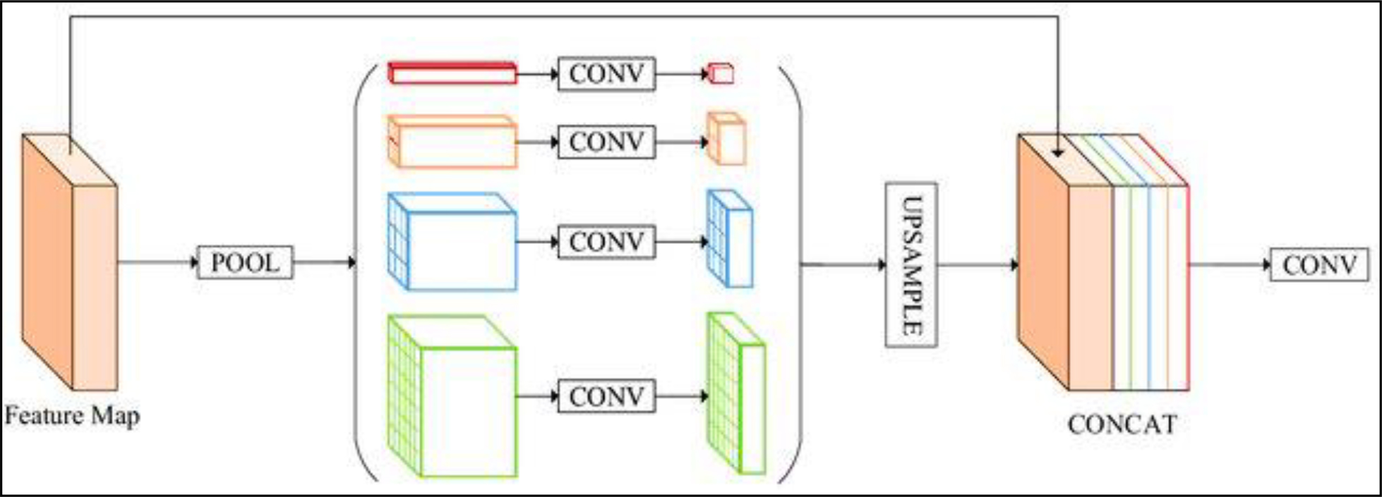

3.3 Training phase: The module for pyramid pool

Pyramids pool was initially shown to CNN in SPP-Net. Pyramids pool eliminates the fixed size limits of CNNs without sacrificing picture location information and is resilient to object deformations. Pyramids pooled produces multi-level map features in PSPNet. The pyramid sharing tool puts those feature maps together to get both local and world background information. According to Fig. 4, the structure of the pool unit in our network contains four pyramidal tiers. We employ volumetric data from 3D pool operations instead of geographic information. Pyramid pooling uses bins with widths of 1* 1* 1*4*4* 8*8 and 16*16 respectively. The various pyramid levels separate the characteristic map into various sub-volumes and get the pooling depiction of features at various points. Every pyramid level has a 1 $\times$ 1 $\times$ 1 convolution layer that works to limit the total amount of streams to 1 4. The low-dimension features is scaled to its initial map of features form using an up sampling layers. The final pyramidal pooled worldwide characteristic is created by concatenating several characteristic layer combinations.

3.3.1 CNN with SPPNet

Our RP-Net design illustrated in Fig. 5, is described here. The RP-Net has two paths – one up sampling along with a downsampling – each of which has four phases, similar to the 3D U-Net.

Figure 5.

Training with SPP-Net’s structure.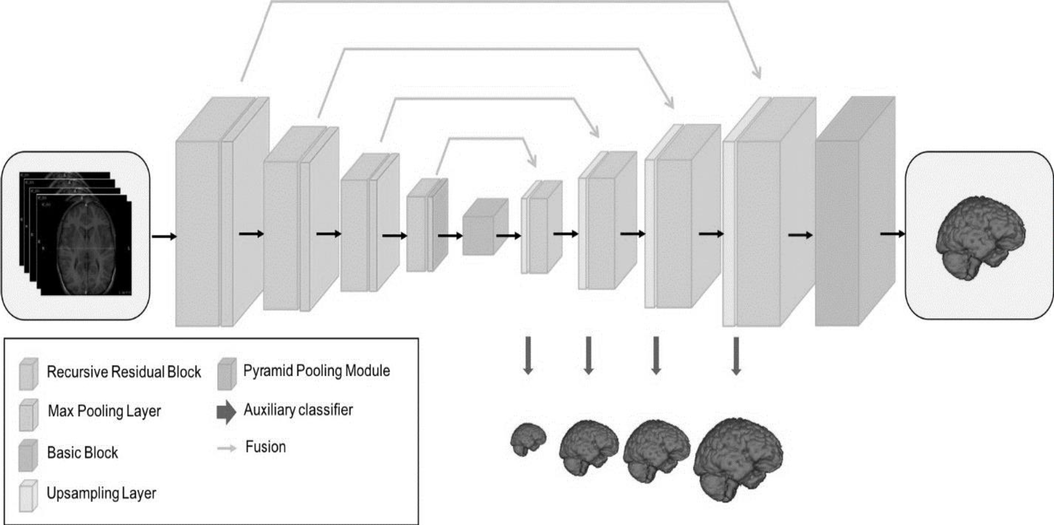

Each level of the down sampling route has a recursion remaining blocks with 3 additional units (Fig. 3(c)) plus a two $\times$ 2 $\times$ 2 maximal pooling level having lengths of 2. The layer of convolution and recursive residual sections constitute new layers that are present at each step of the subsequent samples process. We use the pyramidal pooled element in Fig. 3 to collect volume context-relevant information at the end of the trip. In RP-Net, every neural layer has a 3* 3 *3 filtering kernels. The characteristic mapping is element-wise added before feed to the iterative residue blocks in the upsampling route. Our network uses spatial knowledge by implementing pools, convolutions, and up sampling levels in 3D. We also add a deep supervision technique to the RP-Net to hasten convergence and enrich the concealed layer characteristics. Auxiliary classifiers provide concealed layer monitoring. To produce a characteristic mapping having input equivalent size as the inputs, we utilize an expanding layer, elementwise furthermore, and a 1 *1 *1 convolutional level. Finally, we use a combination level to provide supplemental coarser forecasts. The system’s core predictor is generated via a 1 $\times$ 1 $\times$ 1 convolutional layer. The supplemental loss equation optimizes instruction, but we utilize the main branching for the last predictions throughout validation.

3.4 Details of implementation

The Python-based framework Keras, which supports 3D operations, provides the foundation for our solution.

Figure 6.

Testing flow.

Keras’ default settings randomize the RP-Net without pretraining. We use data enhancement, as described in Subsection II-B, to decrease overfitting. We train the master classification and supplementary classifiers using categories cross-entropy losses. For the four ancillary losses, we set the equilibrium value at 0.2. We select at random 12812848 sub-volumes from every collection to use as input while retraining the algorithm because to the restricted GPU RAM. Only the master branch is used for forecasting during validation. The testing procedure is divided into the two phases seen in Fig. 6. The whole photograph was first uploaded to the website. The stride is 120 *120 *40, while the sub-volume length is 128 *128 *48. The coarse area of relevance is cropped using the end outcome. In the subsequent phase, CLAHE & normalizing are once again applied to the area of interest with the goal to prevent pixel contamination around the brain location. The pace is shorter at 32* 32 *12, and the structure and tactics are identical in the previous level. The median of the likelihood mappings of the sub-volumes in the subsequent phase provides the forecast for the whole end quantity.

Figure 7.

Brain segmented outcomes were analyzed for three datasets: (a) CANDI – BPDwPsy_067 image on axial (128), coronal (64), and sagittal (128) slices, (b) IBSR18 – 10 images on axial (128), coronal (64), and sagittal (128) slices, and (c) IBSR20 – 6_10 image on axial (128), coronal (32), and sagittal (128) slices.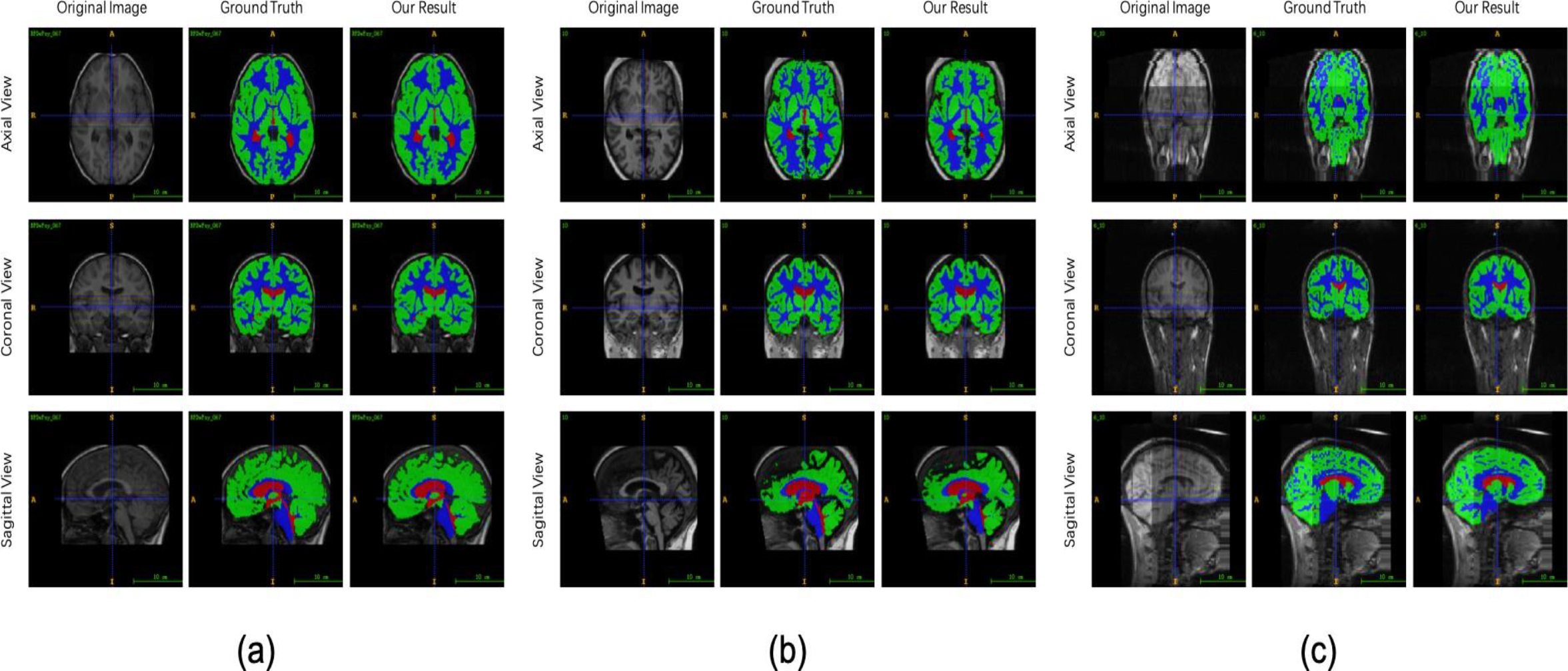

4. Experimental results

DSC is determined by every tissue type (GMs, WMs & CSFs) to evaluate segmentation. Amount of overlap among automated & traditional segmentation is evaluated by the DSC, having an index of 0 to 1. It’s described as

$\displaystyle\textit{DSC}\left({A,M}\right)=\frac{2\left|{A\cap M}\right|}{% \left|A\right|+\left|M\right|}\ast 100\%$ (6)

where $A$ as automated segment outcome and $M$ is human result segment

$\displaystyle\textit{DSC}\left({A,M}\right)=\frac{2\mathop{\sum}\nolimits_{i}^% {N}Piqi|}{\mathop{\sum}\nolimits_{i}^{N}p_{i}^{2}+\mathop{\sum}\nolimits_{i}^{% N}q_{i}^{2}}\ast 100\%$ (7)

When $N$ as entire amount of regional picture, $p_{i}$ & $q_{i}$ , respectively, are the regions used for human and automated segments.

Utilizing the CANDIs & IBSRs databases, 141 photos are used to assess RP-Net’s effectiveness. 61 photos are utilized to create the training data set while 21 pictures were employed to create the validation data set using the CANDI database. The additional 21 photos from the CANDI database as well as the entirety of the IBSR20 & IBSR18 databases are used to enhance the test collection. Table 2 provides a summary of the train, verification, and test set. In our investigations, we use voxelwise categorization for dividing tissue in the brain. The four categories of WM, GM, CSF, and backdrop are applied to each voxel. The framework with the greatest mean DSC rating on the verification set is tested on the test set.

Table 2

Information from training, validating & testing

Sets	Database	#Picture	Modalities
Train	CANDIs	62	T1-Ws
Verification		22
Testing		22
		19
		21

Figure 8.

DSCs bar graphs of the CSFs, GMs, and WMs utilizing the (a) CANDI a database, (b) IBSR18s database (c) IBSR20s database.

4.1 Analysis of the CANDIS & IBSRS database

DSC standard efficiency is displayed in Fig. 7. The mean DSC for CSFs, GMs, and WMs in the CANDI records is 87.88%, 93.47%, and 92.90%, respectively. RP-Net ratings 88.18%, 92.08%, as well as 91.28% on IBSR18 as well as 81.09%, 87.81%, as well as 85.89% on IBSR20 for the same courses. Quantitative figures demonstrate that all three tissues had outstanding accuracy. As might have seen, the normal DSC of CSF, GM, as well as WM have nearest inside IBSR18 as effectively as CANDI the form of databases, but the results on IBSR20 data is the worst of the 3. IBSR20 pictures are more challenging to segment than IBSR18 pictures since many of them have abnormalities and artefacts from the collection process. A few instances of cerebral segmentation outcomes and initial pictures from the three datasets are shown in Fig. 7. These findings show that our technique successfully segments brain tissues when viewed from a visual perspective.

Table 3
DSCs of IBSR18 including IBSR20’s CSFs, GMs, WMs, and their averages

Models	IBSR18s				IBSR20s
	CSFs in %	GMs in %	WMs in %	Mean in %	CSFs in %	GMs in %	WMs in %	Mean in %
CNN(res)	84.80	92.42	90.42	89.21	63.41	83.10	78.46	76.78
CNN(recur)	87.32	92.73	92.74	90.59	78.98	87.63	85.58	86.01
CNN(recur $+$ ds)	87.46	92.06	92.96	92.07	79.53	88.27	87.58	85.68
SPP-Nets	89.19	92.23	91.90	92.23	82.07	89.93	86.90	86.78

Figure 9.

Bar graphs showing the DSCs for CSFs, GMz, with WMs using four different networks utilizing (a) IBSR18 database and (b) IBSR20 database.

4.2 Ablation analysis on IBSR dataset

Recurrent block residuals with 3 residue components, a pyramidal pooled component, and a deep supervisory system are all components of the SPP-Net. CNN removes deep supervising based on the SPP-Net without pyramidal pool component. Additionally, we switch out the recursion remaining block for the CNN remaining interfere with, as illustrated in Fig. 5. The output of the 4 networks is seen in Fig. 8 and is evaluated over white matter (WM), gray matter (GM), and cerebrospinal fluid (CSF).

Table 4
DSCs of CSFs, GMs, WMs and their combined mean for IBSR18 and IBSR20

Models	IBSR18s				IBSR20s
	CSFs in %	GMs in %	WMs in %	Mean in %	CSFs in %	GMs in %	WMs in %	Mean in %
CNN(res)	84.80	92.42	90.42	89.21	63.41	83.10	78.46	76.78
CNN (recur)	87.32	92.73	92.74	90.59	78.98	87.63	85.58	86.01
CNN (recur $+$ ds)	87.46	92.06	92.96	92.07	79.53	88.27	87.58	85.68
SPP-Nets	89.19	87.36	85.96	75.39	82.07	87.98	89.94	87.78

Figure 10.

Outcomes of classification using various deeper supervised levels (axial viewpoint). The initial image is in (a), the fundamental reality is in (b), and the separated outcomes of the deep supervised layers are in (c) to (f).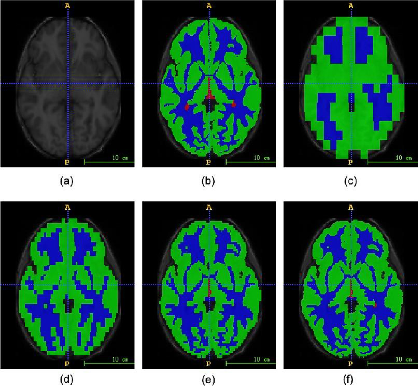

4.3 Effeciency of recurrent residual phase

Evaluate the recurrent residue block, we evaluate the suggested approach to one that does not include it. CNNrecur and CNNres are taught the exact same way. Both of them have U-Net architecture. CNNres has steps with the remaining block in which every unit’s input is the output of the preceding device, whereas CNNrecur includes steps having the recursive residue blocks that each unit’s intake is the outcome of the block’s first fourier level. According to the findings of Table 3, CNNrecur outperforms CNNres, improving the median DSC on the IBSR18 and IBSR20 datasets by 1.38% and 9.03%, respectively.

4.4 Performance of the pyramid pool phase

As demonstrated in Table 3, our system with pyramids pool modules improved the mean DSC for IBSR18 and IBSR20 by 0.68% and 0.92%, correspondingly. In comparison to CNNrecur $+$ ds, PR-Net outperforms it when it comes to CSF division, improving mean DSC on IBSR18 & IBSR20 by 1.73% and 2.54%, respectively, whereas WM’s mean DSC on IBSR20 only decreased by 0.44%.

4.5 Results of supervision in deep

We contrast CNN’s performance with and without extensive monitoring. CNNrecur has no auxiliary classification algorithms, whereas CNNrecur $+$ ds does. In comparison to CNNrecur, the median DSC of CNNrecur $+$ ds improves 0.23% on IBSR18 and 1.03% on IBSR20. Additionally, CNNrecur+ds improves on the average DSC of WM by 1.87%.

4.6 Comparison with other methods on IBSR dataset

Much research on segmenting brain regions have made substantial use of the IBSR database. Table 4 highlights some of the research that used the IBSR database as a baseline for categorization and their findings when applied to the IBSR database. They test their approach using some or all if the information. Our outcomes are profitable, as may be observed. We evaluate our RP-Net with 3 segmented approaches, 3D U-Net, 3D-like FCN [24], and VoxResNet, utilizing the identical training and verification set. U-Net is often utilized in the classification of medical photos. The 3D U-Net architecture that we examined is described above. The greatest result out of the single-modality approaches in the MRBrains13 contest was recorded by the 2.5D CNN known as the 3D-like FCN.

A key technique in the MRBrains13 contest is VoxResNet. We only utilize one method, therefore T1-weighted images are the only ones we use to assess the design of VoxResNet. CSF, GM, & WM categorization efficiency on the IBSR18 and IBSR20 datasets is shown in Table 4. With improvements of 1.85%, 1.69%, and 4.54% on the median DSC. Furthermore, we outperform the three techniques as measured against the IBSR20, with increases in performance of 7.32, 3.12, and 6.19%.

5. Conclusion

To offer a comprehensive solution for the precise and efficient diagnosis and management of Alzheimer’s disease (AD), the proposed comprehensive framework integrates multiple methodologies, including preprocessing, denoising, segmentation, classification, and chatbot recommendation. This framework encompasses various algorithms such as Multilayer Perceptron (MLP) for preprocessing, Ant Colony Optimization (ACO) for denoising, U-Net for segmentation, and Spatial Pyramid Pooling Network (SPPNet) for classification. Incorporating the recursive residual block, pyramid pooling module, and deep supervision method enhances the performance of the network. The robustness of our approach has been evaluated using the CANDI and IBSR datasets. Notably, our method surpasses previous techniques when using a single-modality approach, resulting in highly competitive outcomes in brain segmentation on the IBSR dataset. Specifically, in CSF, GM, and WM, our technique achieves mean DSC values of 88.18%, 92.08%, and 91.21% on the IBSR18 dataset, and 81.06%, 87.91%, and 85.89% on the IBSR20 dataset, outperforming contemporary methods like 3D U-Net, 3D-like FCN, and VoxResNet in terms of segmentation accuracy. These findings underscore the potential therapeutic applications of our proposed automatic brain tissue segmentation architecture.

In future works, incorporating additional clinical information, such as cognitive scores or genetic markers, can provide a more comprehensive understanding of AD and further improve the prediction models. Combining imaging data with clinical and genetic data may facilitate the development of personalized diagnostic and treatment strategies.

References

Grimmer

Henriksen

Wester

Förstl

Klunk

Mathis

Kurz

Drzezga

. Clinical severity of Alzheimer’s disease is associated with PIB uptake in PET. Neurobiology of Aging. 2009 Dec 1; 30(12): 1902-9.

Khalid

Senan

Al-Wagih

Ali Al-Azzam

Alkhraisha

. Automatic Analysis of MRI Images for Early Prediction of Alzheimer’s Disease Stages Based on Hybrid Features of CNN and Handcrafted Features. Diagnostics. 2023 May 8; 13(9): 1654.

Duchesne

Caroli

Geroldi

Barillot

Frisoni

Collins

. MRI-based automated computer classification of probable AD versus normal controls. IEEE Transactions on Medical Imaging. 2008 Mar 31; 27(4): 509-20.

Goren

Montgomery

Kahle-Wrobleski

Nakamura

Ueda

. Impact of caring for persons with Alzheimer’s disease or dementia on caregivers’ health outcomes: findings from a community based survey in Japan. BMC geriatrics. 2016 Dec; 16(1): 1-2.

Eisenmenger

Peret

Famakin

Spahic

Roberts

Bockholt

Johnson

Paulsen

. Vascular contributions to Alzheimer’s disease. Translational Research. 2023 Apr 1; 254: 41-53.

Piller

. Blots on a field? Science (New York, NY). 2022 Jul 21; 377(6604): 358-63.

Mayeux

. Early Alzheimer’s disease. New England Journal of Medicine. 2010 Jun 10; 362(23): 2194-201.

Jicha

Parisi

Dickson

Johnson

Cha

Ivnik

Tangalos

Boeve

Knopman

Braak

Petersen

. Neuropathologic outcome of mild cognitive impairment following progression to clinical dementia. Archives of Neurology. 2006 May 1; 63(5): 674-81.

Gaugler

James

Johnson

Reimer

Solis

Weuve

Buckley

Hohman

. 2022 Alzheimer’s disease facts and figures. Alzheimers & Dementia. 2022 Apr 1; 18(4): 700-89.

10.

Kim

Jeong

Stiles

Choi

. Neuroimaging modalities in Alzheimer’s disease: diagnosis and clinical features. International Journal of Molecular Sciences. 2022 May 28; 23(11): 6079.

11.

Díaz

Mesa-Herrera

Marín

. DHA and its elaborated modulation of antioxidant defenses of the brain: Implications in aging and AD neurodegeneration. Antioxidants. 2021 Jun 3; 10(6): 907.

12.

Vaisvilaite

Hushagen

Grønli

Specht

. Time-of-day effects in resting-state functional magnetic resonance imaging: Changes in effective connectivity and blood oxygenation level dependent signal. Brain Connectivity. 2022 Aug 1; 12(6): 515-23.

13.

Jung

Sung

Nayak

Kim

. k-t FOCUSS: a general compressed sensing framework for high resolution dynamic MRI. Magnetic Resonance in Medicine: An Official Journal of the International Society for Magnetic Resonance in Medicine. 2009 Jan; 61(1): 103-16.

14.

Protonotarios

Tzampazidou

Kastis

Dikaios

. Discrete Shearlets as a Sparsifying Transform in Low-Rank Plus Sparse Decomposition for Undersampled (k, t)-Space MR Data. Journal of Imaging. 2022 Jan 29; 8(2): 29.

15.

Gorges

Müller

Kassubek

. Structural and functional brain mapping correlates of impaired eye movement control in parkinsonian syndromes: a systems-based concept. Frontiers in Neurology. 2018 May 7; 9: 319.

16.

Afzal

Maqsood

Nazir

Khan

Aadil

Awan

Mehmood

Song

. A data augmentation-based framework to handle class imbalance problem for Alzheimer’s stage detection. IEEE Access. 2019 Aug 5; 7: 115528-39.

17.

Dukart

Mueller

Barthel

Villringer

Sabri

Schroeter

, Alzheimer’s Disease Neuroimaging Initiative. Meta-analysis based SVM classification enables accurate detection of Alzheimer’s disease across different clinical centers using FDG-PET and MRI. Psychiatry Research: Neuroimaging. 2013 Jun 30; 212(3): 230-6.

18.

Seixas

Zadrozny

Laks

Conci

Saade

. A Bayesian network decision model for supporting the diagnosis of dementia, Alzheimer’s disease and mild cognitive impairment. Computers in Biology and Medicine. 2014 Aug 1; 51: 140-58.

19.

Liu

Song

Cai

Pujol

Kikinis

Wang

Feng

. Multifold Bayesian kernelization in Alzheimer’s diagnosis. In Medical Image Computing and Computer-Assisted Intervention – MICCAI 2013; 16th International Conference, Nagoya, Japan, September 22–26, 2013, Proceedings, Part II 16 2013 (pp. 303-310). Springer Berlin Heidelberg.

20.

Zhao

Chan

Tang

Chow

Wong

. Trace ratio linear discriminant analysis for medical diagnosis: a case study of dementia. IEEE Signal Processing Letters. 2013 Mar 7; 20(5): 431-4.

21.

Padilla

López

Górriz

Ramirez

Salas-Gonzalez

Alvarez

. NMF-SVM based CAD tool applied to functional brain images for the diagnosis of Alzheimer’s disease. IEEE Transactions on Medical Imaging. 2011 Sep 12; 31(2): 207-16.

22.

Papakostas

Savio

Graña

Kaburlasos

. A lattice computing approach to Alzheimer’s disease computer assisted diagnosis based on MRI data. Neurocomputing. 2015 Feb 20; 150: 37-42.

23.

Phong

Duong

Nguyen

Trong

Nguyen

Van Hoa

Snasel

. Brain hemorrhage diagnosis by using deep learning. In Proceedings of the 2017 International Conference on Machine Learning and Soft Computing 2017 Jan 13 (pp. 34-39).

24.

Wang

Shen

Chen

Xiao

. Automatic recognition of mild cognitive impairment from MRI images using expedited convolutional neural networks. In Artificial Neural Networks and Machine Learning–ICANN 2017: 26th International Conference on Artificial Neural Networks, Alghero, Italy, September 11–14, 2017, Proceedings, Part I 26 2017 (pp. 373-380). Springer International Publishing.

25.

Aderghal

Khvostikov

Krylov

Benois-Pineau

Afdel

Catheline

. Classification of Alzheimer disease on imaging modalities with deep CNNs using cross-modal transfer learning. In 2018 IEEE 31st international symposium on computer-based medical systems (CBMS) 2018 Jun 18 (pp. 345-350). IEEE.

26.

Schmitter

Roche

Maréchal

Ribes

Abdulkadir

Bach-Cuadra

Daducci

Granziera

Klöppel

Maeder

Meuli

. An evaluation of volume-based morphometry for prediction of mild cognitive impairment and Alzheimer’s disease. NeuroImage: Clinical. 2015 Jan 1; 7: 7-17.

27.

Preethi

Asokan

. Neural network oriented roni prediction for embedding process with hex code encryption in dicom images. In Proceedings of the 2nd International Conference on Advances in Computing, Communication Control and Networking (ICACCCN), Greater Noida, India 2020 Dec (pp. 18-19).

28.

Preethi

Asokan

Thillaiarasu

Saravanan

. An effective digit recognition model using enhanced convolutional neural network based chaotic grey wolf optimization. Journal of Intelligent & Fuzzy Systems. 2021 Jan 1; 41(2): 3727-37.

29.

Ganesh

Kumar

Reddy

Kavitha

Murthy

. Implementation of AI Pop Bots and its allied Applications for Designing Efficient Curriculum in Early Childhood Education. International Journal of Early Childhood Special Education. 2022 May 1; 14(3).

30.

Asokan

Preethi

. Deep learning with conceptual view in meta data for content categorization. In Deep Learning Applications and Intelligent Decision Making in Engineering. 2021; (pp. 176-191). IGI Global.

31.

Prasad

Turukmane

Kumar

Madhavi

Sushama

Neelima

. Cnn Based Pathway Control To Prevent Covid Spread Using Face Mask And Body Temperature Detection. Journal of Pharmaceutical Negative Results. 2022 Oct; 5: 1374-81.

32.

Bai

Preethi

. Security enhancement of health information exchange based on cloud computing system. International Journal of Scientific Engineering and Research. 2016 Oct; 4(10): 79-82.

33.

Malchi

Kallam

Al-Turjman

Patan

. A trust-based fuzzy neural network for smart data fusion in internet of things. Computers & Electrical Engineering. 2021 Jan 1; 89: 106901.

34.

Sangamithra

Neelima

Kumar

. A memetic algorithm for multi objective vehicle routing problem with time windows. In 2017 IEEE International Conference on Electrical, Instrumentation and Communication Engineering (ICEICE) 2017 Apr 27 (pp. 1-8). IEEE.

35.

Sunil Kumar

Rama Mohan Reddy

. An Efficient Approach for Evolution of Functional Requirements to Improve the Quality of Software Architecture. In Artificial Intelligence and Evolutionary Computations in Engineering Systems: Proceedings of ICAIECES. 2015; 2016 (pp. 775-792). Springer India.

An effectual recommendation model using hybrid learning models for early detection of Alzheimer’s disease

Abstract

Keywords

1. Introduction

Table 1 Review on ADs forecasting techniques in existing researches

3.1 Data pre-processing

3.1.1 Multilayer perceptron (MLP)

3.1.2 Ant colony optimization (ACO)

3.1.3 Mathematical formulation

3.2.2 Recurring block of residual

3.3.1 CNN with SPPNet

Table 3 DSCs of IBSR18 including IBSR20’s CSFs, GMs, WMs, and their averages

Table 4 DSCs of CSFs, GMs, WMs and their combined mean for IBSR18 and IBSR20

4.4 Performance of the pyramid pool phase

4.5 Results of supervision in deep

4.6 Comparison with other methods on IBSR dataset

5. Conclusion

References

Table 1
Review on ADs forecasting techniques in existing researches

Table 3
DSCs of IBSR18 including IBSR20’s CSFs, GMs, WMs, and their averages

Table 4
DSCs of CSFs, GMs, WMs and their combined mean for IBSR18 and IBSR20