Hybrid LSTM models-based detection of left ventricular hypertrophy in electrocardiogram signals

Abstract

This research investigates various deep learning techniques to automatically classify Left Ventricular Hypertrophy (LVH) from electrocardiogram (ECG) signals. LVH frequently results from persistently high blood pressure, causing the heart pump harder and thicken the ventricular walls. It is associated with an increased risk of heart attacks, heart failure, stroke, and sudden cardiac death. The significance of this research lies in the early and precise detection of LVH, facilitating timely interventions and ultimately improving patient health. The non-invasive nature of ECG monitoring, integrated with the efficiency of deep learning models, contributes to faster and more accessible to enhance diagnostic accuracy and efficiency in identifying LVH. The objective of this research is to assess and compare the performance of GRU3Net, Double-Bilayer LSTM, and Conv2LSTM, Dual-LSTM models in the classification of Left Ventricular Hypertrophy (LVH) based on electrocardiogram (ECG) signals, utilizing a dataset sourced from the PTB Diagnostic ECG Database. The implemented deep learning models yielded noteworthy results. Specifically, the GRU3Net model achieved a high accuracy of 96.1%, showcasing an optimal configuration for overall accuracy. The Double-Bilayer LSTM model followed with an accuracy of 91.7%. However, a decline in accuracy was observed in both the Dual-LSTM and Conv2LSTM models, with the former registering an accuracy of 90.8% and the latter decreasing further to 87.3%.

Keywords

Left ventricular hypertrophy GRU3Net Dual-LSTM Double-Bilayer LSTM Conv2LSTM model

1. Introduction

According to statistics, cardiovascular diseases (CVDs) were the primary cause of 17.7 deaths worldwide in 2017 [1]. Patients with hypertension could exhibit signs of left ventricular hypertrophy, which increases the chance of developing heart failure with congestion and asymptomatic dysfunction of the left ventricle (LV) [2, 3]. Prolonged high blood pressure develops adaptive reactions in the heart and blood arteries to lessen the burden. These modifications include the left ventricle’s remodeling and the thickening of blood vessel walls [4, 5]. Left Ventricular Hypertrophy (LVH) indicates a substantial increase in the mass of the left ventricle. This condition frequently leads to aortic heart disease, mitral valve insufficiency, arterial hypertension (AH), and other conditions that expose the Left Ventricle (LV) to prolonged stress and overload [6]. LVH is an indicator for the development of heart failure (HF) and sudden mortality, as well as a unique cardiac disease in people with arterial hypertension (AH).

Moreover, patients with increased ventricular mass have a higher chance of death from cardiovascular disease (15%) and from all causes (16.5%) [7]. LVH is most frequently caused by hypertension and aortic valve stenosis. The heart is beating against an increased afterload in each of these situations. An additional reason is left ventricular diastolic overload caused by increased filling, which is the fundamental mechanism behind eccentric left ventricular hypertrophy (LVH) in individuals with regurgitant valvular diseases such as aortic or mitral regurgitation, as well as in patients with dilated cardiomyopathy.

The pathophysiology of left ventricular hypertrophy (LVH) has been demonstrated to incorporate coronary artery disease (CAD) as the myocardium undergoes compensatory changes in response to ischemia or infarcted tissue. Physiological Left Ventricular Hypertrophy in athletes is a rather mild condition. Extensive exercise increases the size, thickness, and muscle mass of the left ventricle, but does not affect the diastolic or systolic function. The 15% to 20% of people in the general population have left ventricular hypertrophy (LVH) [8]. Studying 37700 people’s echocardiography data, it was shown that in untreated hypertensives, the prevalence of LVH ranged from 19% to 48%, and in high-risk hypertensive patients, it ranged from 58% to 77%.

Additionally, obesity increases the chance of LVH development by two times. Depending on whether definitional criteria are applied, the prevalence of LVH in the population varies from 36% to 41%. Male and female rates of LVH prevalence are reported to be in an equal range of 36.0% against 37.9% and 43.5% versus 46.2%. Compared to concentric hypertrophy, eccentric LVH is comparatively more common. However, if pathologic LVH develops, the patient is far more likely to experience dysrhythmias, heart failure, and unexpected death. An additional reason is left ventricular diastolic overload caused by increased filling, which is the fundamental mechanism behind eccentric left ventricular hypertrophy (LVH) in individuals with regurgitant valvular diseases and dilated cardiomyopathy disease. Myocardial fibrosis is developing along with LVH, which is a significant pathophysiologic component. Systolic dysfunction can also develop with increasing illness, but diastolic dysfunction is the initial clinical manifestation of fibrosis [9].

Concentric hypertrophy and eccentric hypertrophy are two distinct forms of left ventricular hypertrophy, characterized by variations in relative wall thickness (RWT) and left ventricular mass (LVM) index. The concentric hypertrophy is identified by an increased LWM index and RWT exceeding 0.42, while eccentric hypertrophy is characterized by an elevated LWM index and RWT less than or equal to 0.42. These distinctions are based on measurements involving the posterior wall thickness, left ventricular internal diameter at end-diastole, and normalization of left ventricular mass for body surface area or height.

Concentric left ventricular hypertrophy denotes an abnormal elevation in the mass of the left ventricle due to sustained strain on the heart. It is commonly induced by pressure overload resulting from arteriolar vasoconstriction, a phenomenon observed in conditions such as aortic stenosis or chronic hypertension. Diastolic overload, also known as volumetric or diastolic overload, is the underlying mechanism for patients with regurgitant valve lesions. It increases the left ventricle’s filling pressure, which results in eccentric left ventricular hypertrophy. These pathways may contribute to an attempt by individuals with coronary artery disease to make up for myocardial tissue that has been ischemia or infarcted [9].

1.1 ECG criteria on LVH

The evaluating of the LVM is also perceived in the ECG signal. In cases where the amplitude of the QRS complex varies and the increased LVM agrees, the outcomes are classified as true positives, signifying the minority of LVH cases. These findings are labeled as false negatives if there is a discrepancy. The flaw in this strategy was shown by Pevsner’s meta-analysis, which revealed a broad range of sensitivity and specificity for the ECG-LVH criteria [10, 11]. An even more intricate ECG-LVH criterion that takes into account irregularities in the ECG other than only elevated voltage is the Romhilt-Estes score (R–E) [11]. The risk of ventricular arrhythmia is exacerbated by the higher QRS complex amplitude [11, 12]. However, the predicted risk is also lower since the overall rate of ECG-LVH is lesser than the LVH found by using echocardiography [13, 14].

1.2 ECG findings in LVH patients

Among patients affected with Left Ventricular Hypertrophy (LVH), there is a diversity of QRS patterns, with elevated QRS voltage being just one manifestation. The sensitivity of this particular pattern varies from 0% to 60% and it is seen in a small percentage of LVH cases [15]. Patients with Left Ventricular Hypertrophy (LVH) exhibit leftward movement of the electrical axis in the frontal plane, longer QRS duration, and alterations in the ST segment and T wave in addition to increased QRS amplitude. Intraventricular conduction abnormalities are common and include incomplete Left Anterior Fascicular Block (LAFB), Left Bundle Branch Block (LBBB), and Left Bundle Branch Block (LBBB). False-negative results can occur in the form of apparently normal QRS complexes. Research has shown that the anatomical type of left ventricular hypertrophy (LVH) and an augmented Left Ventricular Mass (LVM) are not the important factors influencing the QRS complex. It has been established that an elevation in LVM does not necessarily lead to a rise in the amplitude of the QRS. The widespread reduction in conduction velocity, combined with various anatomical types of left ventricular hypertrophy (LVH), brings about alterations in QRS amplitude, duration, and morphology.

The intriguing influence of anatomical modifications and changes in conduction velocity on the varied clinical ECG-left ventricular hypertrophy (LVH) criteria [16]. The changes in the shape of the QRS complex structure that are typically realized as the consequence of left ventricular hypertrophy, or the enlargement of the LV mass [16, 17, 18].

2. Literature survey

In recent decades, there has been a notable surge in the adoption of deep learning-based approaches for the classification of heart diseases, reflecting a prominent trend in cardiovascular disease research [19, 20]. The various successful applications include the detection of atrial fibrillation, ECG arrhythmia, myocardial infarction, Left Ventricular Hypertrophy, premature ventricular contraction beats, and the classification of ECG diseases in comparison to healthy patients [21, 22]. These achievements have been realized through the utilization of deep neural networks and conventional machine learning algorithms [23]. Deep learning, a subset of machine learning, diverges from traditional machine learning approaches by seamlessly incorporating feature extraction and classification within its hidden layers. Unlike conventional methods where external researchers explicitly handle these tasks, deep learning networks autonomously perform these functions internally, streamlining the process [42].

Xiaoli Zhao et al. leveraged the Convolutional Neural Network (CNN) in conjunction with the Long Short-Term Memory (LSTM) model, demonstrating their efficacy as optimal architectures for classification [24]. Remarkably, the CNN-LSTM model proved highly effective in forecasting Left Ventricular Hypertrophy (LVH), attaining an Area Under the Curve (AUC) of 0.62, along with a sensitivity of 68% and a specificity of 57%. Notably, the model consistently demonstrated robust performance, maintaining an AUC of 0.59, with a sensitivity of 65% and specificity of 57% for overall LVH prediction. In subgroup analysis, the CNN-LSTM model excelled in predicting LVH through 12-lead ECG, particularly for male patients, achieving an impressive AUC of 0.66 with a sensitivity of 72% and specificity of 60%. This performance surpassed that observed for female patients, where the AUC was 0.59, sensitivity was 50%, and specificity was 71%[24].

Khurshid S. et al. pioneered the development of a Convolutional Neural Network (CNN) specifically employed on the complete 10-second 12-lead ECG waveform to predict left ventricular (LV) mass [25].

Jimmy Ming et al. introduced a six-layer deep neural network, specifically crafted for this study, aimed at predicting left ventricular hypertrophy. Overfitting was avoided by using L2-regularization and dropout strategies in every model iteration. The system, aptly named the Electrocardiographic Left Ventricular Hypertrophy Classifier (ELVHC), exhibited notable performance in experimental findings. The precision of the forecast model reached 73%, sensitivity stood at 66%, and specificity achieved an impressive 78%. These results significantly outperformed two clinical techniques, highlighting the efficacy of the ELVHC in predicting left ventricular hypertrophy [26].

To assess the efficacy of AI-enabled analysis of the 12-lead electrocardiogram (ECG) in automating the identification and classification of left ventricular hypertrophy (LVH), Julian et al. introduced the LVH-Net model, and the performance, as indicated by the areas under the receiver operator characteristic curve (AUC), varied among distinct Left Ventricular Hypertrophy (LVH) etiologies. The AUC for cardiac amyloidosis reached 0.95, for hypertrophic cardiomyopathy it was 0.92, for aortic stenosis LVH it stood at 0.90, for hypertensive LVH it was 0.76, and for other LVH cases, it reached 0.69.

These results underscore the effectiveness of the LVH-Net model, as introduced by Julian and colleagues, in discriminating various LVH etiologies. Noteworthy, the single-lead models also exhibited robust discrimination capabilities [27].

Joon-Myoung Kwon et al. introduced an artificial intelligence (AI) algorithm utilizing an ensemble neural network (ENN) that combined convolutional and deep neural network architectures. This innovative algorithm, trained on a derivation dataset, aimed to detect LVH. The research included the visualization of specific ECG areas crucial for the AI algorithm’s decision-making process. The area under the receiver operating characteristic curve (AUC) for the AI algorithm based on ENN reached 0.880. Notably, this AI algorithm, rooted in ENN, demonstrated exceptional efficacy in LVH detection, surpassing the performance of cardiologists, traditional methods, and other machine-learning techniques [28, 63].

An RNN neural network specifically crafted for capturing patterns in sequential data, including but not limited to event sequences, time series, and natural language. It performs by using the previous step’s output as the subsequent step’s input. Through the continuous adjustment of hidden units and memory, an RNN indicates the capability to retain information sequentially. Specifically for ECG data, RNNs emerge as a choice because of their ability to effectively capture temporal dependencies and accommodate inputs of varying lengths. Commonly employed RNN variants for this purpose include bidirectional-LSTM (BiLSTM) and GRU/LSTM models, which address the significant challenge of vanishing gradients, a limitation observed in classical RNNs. In a study referenced as [29], two compact LSTM networks were utilized to amalgamate raw ECG date and wavelet transform (WT) features, enabling continuous execution in real time on wearable devices. Another study denoted as [30], introduced an attention mechanism into a BiLSTM network to visualize attention weights and improve performance and interpretability.

The CRNN integrates CNN with RNN modules, presenting an advantageous architecture for effectively handling extended ECG signals characterized by various sequence lengths and multi-channel inputs. Utilizing either a 1-dimensional CNN [31] or a 2Dimensional CNN [32], the CRNN extracts features from the ECG sequence. Subsequently, an RNN combines these local features along with the temporal dimension, generating global features.

The cardiovascular risk estimation from heart rate patterns generated from ECG data [33] adopts the CRNN framework. For the purpose of rendering interpretable diagnoses, integrates a CRNN with a multi-level attention system [34]. This mechanism incorporates rhythm-level, beat-level, and frequency-level features that utilize medical domain knowledge, contributing to a comprehensive and nuanced understanding of the diagnostic process [35].

A neural network framework known as a Generative Adversarial Network (GAN), pioneered by Goodfellow et al. [36], comprises two distinct sub-models: a generative model (G), responsible for capturing the latent representation of the data distribution within a training dataset, and a discriminative model (D), tasked with assessing the likelihood that a generated sample originates from the authentic data distribution. Through an iterative training process, these two models engage in a minimax game. GANs have recently been employed to address the data imbalance challenge in ECG data. In [37], the authors introduced an abnormality detection model for ECG signals based on a CRNN framework. They incorporated a GAN consisting of multiple 1D CNNs for data augmentation, leading to excellent performance on class-imbalanced datasets. Another application is found in [38], where a GAN was utilized for denoising ECG data. Furthermore, in [39], a GAN was proposed with a generator made of a BiLSTM network and a discriminator comprising a CNN. This GAN was employed to generate synthetic ECG data for training a deep-learning model [40].

3. Dataset

The study utilized ECG data 12-lead PTB Diagnostic ECG Database. To ensure consistency in sampling frequencies, signals from the St. Petersburg Diagnostic databases were up-sampled to 1000 Hz [64]. Subsequently, the ECG signals were partitioned into segments, each representing a 2-second window length containing 2000 samples. In this, 540 segments represent LVH signal remaining represents normal segments. Figures 1 and 2 depicts the ECG signal with LVH and normal ECG signal.

Figure 1.

ECG signal with LVH.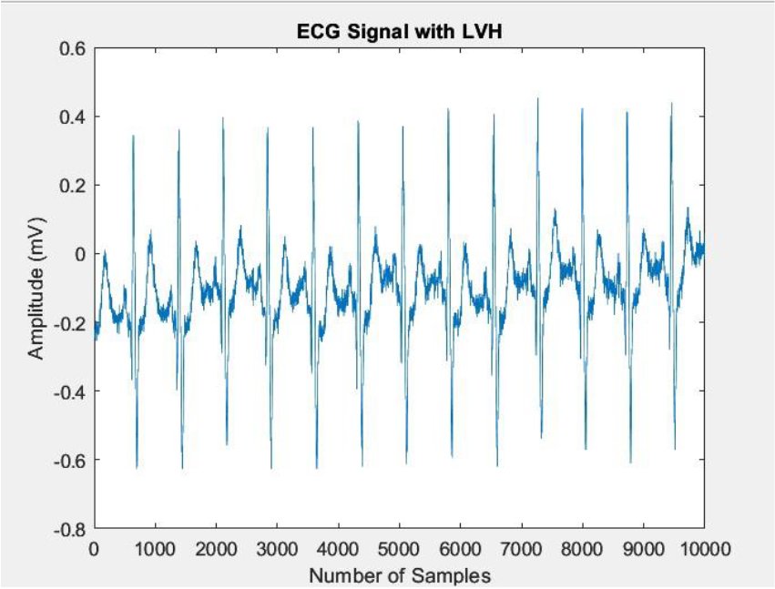

Figure 2.

Normal ECG signal.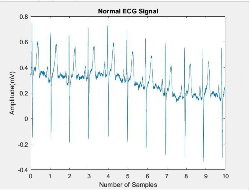

3.1 Imbalance dataset

The Imbalanced label distributions are a common challenge in ECG disease classification, often characterized by the infrequent occurrence of severe diseases that hold significant clinical importance. This rarity poses difficulties in training deep learning models effectively, especially when dealing with a limited dataset for disease labels. Two primary approaches exist to address this issue which includes the data augmentation techniques, such as preprocessing or the creation of synthetic training datasets using generative models [51, 52, 53].

In this study, data augmentation using circular shift with a shift amount of 5 is implemented in order to enhance the deep learning model’s performance. This significant shift in the ECG signals aids in the generation of enhanced samples without distorting important aspects such as the QRS complex, which is essential for the diagnosis of LVH. For a 1-dimensional data sample $x$ , the circular shift can be performed using the following formula:

$\displaystyle x^{\prime}_{i}=x_{i+s}\textit{ mod }N$ (1)

where $N$ is the length of $x$ , $s$ is the shift amount, and circularly shifted sample ${x}^{\prime}_{i}$ . In total, the study incorporated 4080 such segments.

4. Materials and methodology

In recent decades, deep learning has been an effective tool for effective data analysis. The integration of artificial neural networks in deep learning has significantly enhanced the processing of sequential data tasks, such as speech recognition, language translation, signal, and image classification. This improvement is attributed to the remarkable feature learning capabilities of neural networks, enabling them to comprehend complex datasets. State-of-the-art neural networks excel at making predictions directly from raw data inputs, elevating the efficiency of data analyses and eliminating the necessity for expert knowledge. The purely data-driven nature of these algorithms ensures that their performance accuracy scales with increasing amounts of data, underscoring their adaptability and effectiveness [41]. Figure 3 shows the block diagram of the proposed model.

Figure 3.

Block diagram of proposed model.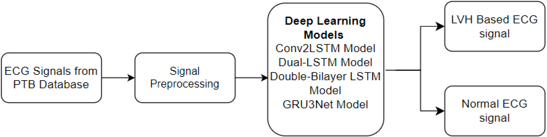

In this study, the ECG data from the PTB database was pre-processed with techniques including sampling and data augmentation. The pre-processed signals were fed into various deep learning models, including Conv2LSTM, Dual-LSTM, Double-Bilayer LSTM, and GRU3Net, to distinguish between ECG signals with LVH and normal ECG signals.

4.1 Conv2LSTM model

In the modeling process, sequential data serves as the input for the system. Figure 4 depicts the block diagram of the proposed Conv2LSTM model. The initial step involves the utilization of a 1D CNN model, which effectively extracts relevant features from the input data. This convolutional neural network architecture excels at discerning patterns within sequential information. Following this, an LSTM layer is incorporated into the framework, specifically developed to capture and learn long-term dependent inherent in the data. The LSTM layer enhances the model’s ability to recognize and understand intricate relationships over extended sequences. Subsequently, a fully connected layer is employed to amalgamate the distinctive features extracted by the preceding layers, culminating in a comprehensive representation. This integrated information is then leveraged for making predictions. Finally, to convert the fully connected layer output into a meaningful probability distribution over different classes, a softmax layer is applied. The softmax layer ensures that the model’s predictions are transformed into a probabilistic framework, facilitating the interpretation and classification of the sequential data into distinct classes.

Figure 4.

Block diagram of proposed Conv2LSTM model.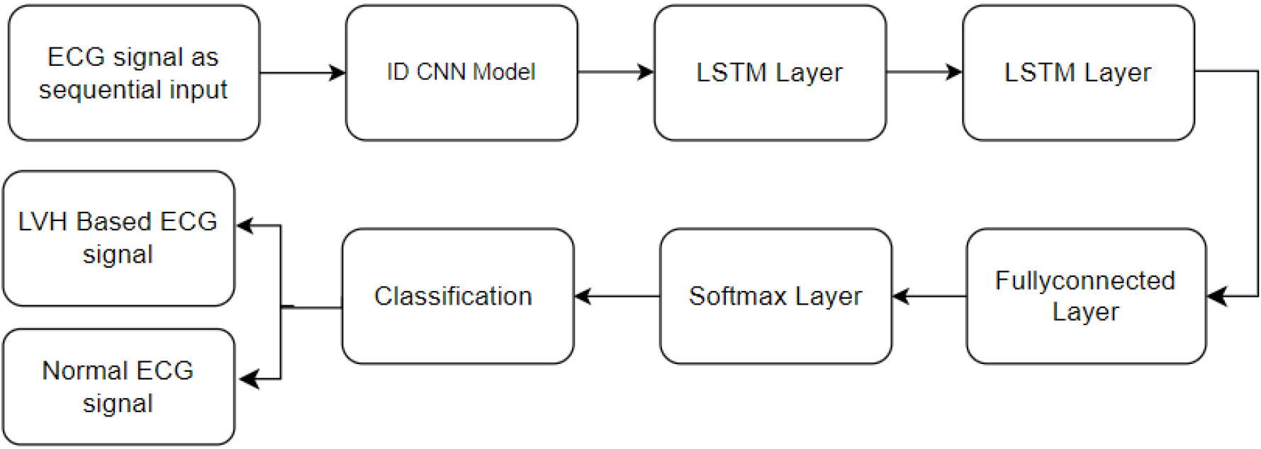

In studies related to CNN2LSTM-based LVH classification, models are constructed with varying depths, based on different layers [39, 42]. This network is designed to process a time series of ECG signals as input data, yielding a sequence of label predictions as its output. These models exhibit a hierarchical structure, featuring convolutional layers for obtaining feature maps, which are subsequently sub-sampled through pooling layers. Following the convolutional layer, a pooling layer is incorporated due to its capability to make the representation roughly invariant to small input translations, as indicated by reference [52]. Furthermore, pooling layers help to decrease the dimensionality of the data. This reduction proves advantageous in preventing overfitting and diminishing computational requirements, thereby facilitating a faster training process for the model.

The 1D convolution function within the convolutional layer was calculated based on the following expression [46].

$\displaystyle x=f\left({b+\mathop{\sum}\limits_{i=1}^{N}\ast({w,y})}\right)$ (2)

The expression involves several components: $x$ represents the complete feature map, $b$ denotes bias, $y$ corresponds to a feature map, $w$ represents the convolutional kernel, $N$ stands for the number of features, and (*) signifies the convolution vector. Additionally, $f(.)$ is utilized as the activation function in the convolution operation.

In convolutional layers, rectified linear units (ReLU) are preferred over sigmoid as the activation function. This choice is driven by the fact that ReLU addresses the issue of gradient vanishing more effectively compared to sigmoid. Additionally, the use of ReLU reduces computational efforts, enhancing the efficiency of computations in convolutional layers [56]. The dropout layer arbitrarily sets some input vector dimensions to zero with a given probability, and it operates without any trainable parameters. This lack of trainable parameters implies that the layer remains unaltered during the training process. This specific layer proves highly effective in mitigating overfitting, as demonstrated by its substantial impact on numerous benchmark tests outlined in reference [56]. The ultimate fully connected layer, comprising two neurons, is succeeded by a single output layer. This configuration generates a distribution across the two output labels. The output layer uses softmax as its activation function for classification. The expression is [56]

$\displaystyle y(z)=\frac{e_{i}^{z}}{\mathop{\sum}\nolimits_{j}e_{i}^{z}}$ (3)

Throughout the training process, the optimization of parameters was carried out using Adam optimizers [57]. The model exhibiting the optimal performance on the validation set during the optimization process was retained as the best model.

The last stage of the proposed model typically incorporates fully connected layers. To enhance robustness against overfitting, regularization techniques such as dropout and batch normalization are implemented [58, 59, 60, 61]. The integration of these regularization layers contributes to the model’s resilience, promoting more effective learning processes. This is followed by two LSTM layers to get effective results.

4.2 Dual-LSTM model

The model takes a sequence of data as input, often representing a time series such as an electrocardiogram (ECG) signal as shown in Fig. 5. Two LSTM units are stacked sequentially. Recurrent Neural Networks (RNNs) of the LSTM type are made to recognize and retain long-term dependence on sequential input. Memory cells, input gates, forget gates and output gates are components of each LSTM unit, which allows the model to learn and store data over lengthy sequences.

The hidden units of the two LSTM models represent learned features and information from the input sequence. LSTM’s memory cells allow the model to selectively remember and forget information, enhancing its ability to capture long-term dependency. Following the LSTM units, a fully connected layer is incorporated. This layer connects each neuron from the previous layer to every neuron in the current layer. The fully connected layer is responsible for learning complex patterns and representations from the features extracted by the LSTM units. The softmax layer is the model’s last layer. which acts as the output layer. It is responsible for converting the raw model predictions into probability scores associated with each class.

Figure 5.

Block diagram of proposed Dual-LSTM model for LVH classification.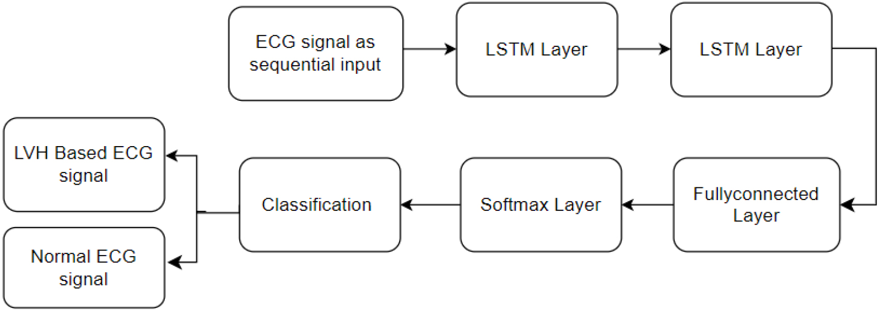

LSTM introduces a modification in recurrent networks through the incorporation of memory blocks. An LSTM structure typically consists of input, hidden, and output layers [43]. Within the hidden layers, specialized memory blocks, referred to as cells, are employed. These cells store information in a gated cell, operating outside the regular flow of the recurrent network. Within the LSTM framework, there are three essential gates which include the input, the output, and the forget gate. These play a pivotal role in regulating the flow of information within the memory cells, collectively forming what is known as a memory cell block. This block consists of identical input and output gates, resembling a structure akin to computer memory where data can be stored comprehensively [44]. The cells, resembling the functions of computer memory, execute these operations by manipulating the gates through an open and close mechanism. These gates, operating in an analog manner, employ a sigmoid function that performs element-wise multiplication, yielding values within the range of 0 to 1. Comparable to nodes in Neural Networks (NN), the gates in LSTM undertake the task of either permitting or inhibiting the passage of information based on signal strength [45].

The model undergoes training using a labeled dataset comprising examples of ECG signals and their corresponding LVH classifications. During training, the model adapts its parameters to minimize the loss function, learning to make accurate predictions.

4.3 LSTM model architecture

Figure 6.

LSTM unit architecture.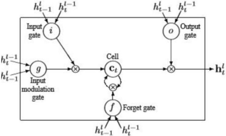

An improved RNN called LSTM has memory cells that improve the learning of data temporal correlations over time. The LSTM concept is built on a memory cell that uses an input gate ( $i_{t}$ ), an output gate ( $o_{t}$ ), and a forget gate ( $f_{t}$ ), to handle the read, write, and reset functions respectively. Every gate functions to retain the information about when and how much the memory’s weights should be updated. The input and output of memory cell activations are regulated by the input and output gates. The following formulas, ranging from 4 to 9, demonstrate the functionality of these gates [46]. The LSTM Model’s architecture is depicted in Fig. 6.

$\displaystyle i_{t}=\sigma(W^{xi}x_{t}+W^{hi}h_{t-1}+b_{i})$ (4) $\displaystyle f_{t}=\sigma({W^{xf}x_{t}+W^{hf}h_{t-1}+b_{f}})$ (5) $\displaystyle o_{t}=\sigma({W^{xo}x_{t}+W^{ho}h_{t-1}+b_{o}})$ (6) $\displaystyle g_{t}=\sigma({W^{xc}x_{t}+W^{hc}h_{t-1}})+b_{c}$ (7) $\displaystyle c_{t}=f_{t.C_{t-1}}+i_{t}g_{t}$ (8) $\displaystyle h_{t}=o_{t.}\varphi({c_{t}})$ (9)

4.4 Double-Bilayer LSTM model

The model takes a sequence of data as input, commonly representing a time series like an ECG signal. Two Bilayer LSTM units are stacked sequentially. Bilayer LSTM is a kind of RNN architecture that incorporates the benefits of LSTM cells. Each Bilayer LSTM unit consists of two LSTM layers stacked on top of each other. The capacity of the model to capture intricate temporal patterns is improved by this stacking. The hidden units of the two Bilayer LSTM represent learned features and information from the input sequence. The architecture of the Bilayer LSTM helps the model retain and utilize information over longer sequences. After the Bilayer LSTM units, a fully connected layer is incorporated. This layer connects each neuron from the previous layer to every neuron in the current layer. Figure 7 illustrates the block diagram of the proposed Double-Bilayer LSTM model for LVH classification.

Figure 7.

Block diagram of proposed Double-Bilayer LSTM model for the LVH classification.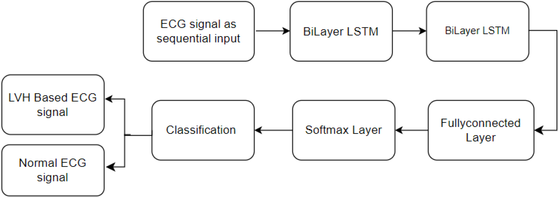

The Bilayer LSTM units extract features, and the fully connected layer uses those features to learn complex patterns and representations. The softmax layer serves as the output layer, it transforms the raw model output into probability scores for each LVH classification.

4.5 Bidirectional LSTM architecture

The Bidirectional Recurrent Neural Network (BRNN) presents a model to overcome limitations inherent in conventional RNNs. This model partitions the states of regular RNN neurons into forward and backward components, essentially comprising two distinct recurrent networks. These networks are linked to a shared output layer, enabling the simultaneous evaluation of past and future contextual information for sequential inputs within a given time frame. This design eliminates delays in processing, allowing for a comprehensive analysis of both preceding and subsequent situations in the input sequence [47]. The LSTM version of the BRNN model is represented by the BLSTM structure. This variant, known as Bidirectional LSTM, offers enhanced performance in classification tasks. In contrast to the conventional LSTM architecture, the BLSTM structure involves the training of two distinct LSTM networks to process sequential inputs. The basic construction of the BLSTM shown in Fig. 8, demonstrates the manner in which it can handle consecutive inputs.

Figure 8.

Bidirectional LSTM architecture.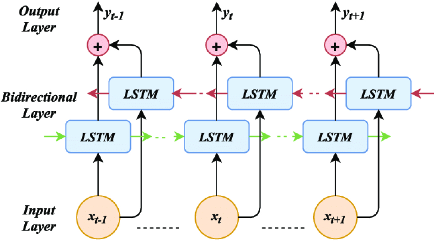

Neurons in a normal unidirectional LSTM structure act similarly to those in the forward state of a Bidirectional LSTM (BLSTM). Significantly, since the neurons in the two networks lack interconnections, in a manner consistent with a conventional unidirectional LSTM, the training of the network can be carried out. These networks generally go through a particular training process in a specific sequence. Bidirectional Recurrent Neural Networks (BRNNs) process input data for each time slice ( $1<t\leqslant T$ ) during the forward pass to produce anticipated outputs.

The forward passes occur sequentially from $t=1$ to $t=T$ , and complementary backward passes from $t=T$ to $t=1$ are conducted. For the output neurons, a forward pass is also performed. In the subsequent backward pass, the derivative of the error function is calculated for every time slice ( $1\leqslant t\leqslant T$ ) that corresponds to the forward pass. This involves backward passes for both the output cells and the forward states, conducted from $t=T$ to $t=1$ and from $t=1$ to $t=T$ , respectively. Subsequently, all weights in the network are adjusted. The effectiveness of BLSTM structures surpassing other network architectures is problem-dependent. Notably, in areas such as speech processing tasks where content holds crucial significance, studies have demonstrated the considerable success of BLSTMs [48, 49].

4.6 GRU3Net model

Three GRU units are stacked one after another as shown in Fig. 9. GRU is a type of RNN that is suited for processing sequential data. Each GRU unit consists of a set of gates which includes an update and reset gate and a hidden unit, allowing the network to acquire and remember temporal dependencies in the input sequence. The hidden states of the three GRU units represent the learned features and information from the input sequence. Following the GRU units, a fully connected layer is employed. Every neuron in the present layer is connected to every other neuron by means of this layer. The fully connected layer is responsible for learning complex patterns and representations from the features extracted by the GRU units. The softmax is the output layer of the model. It converts the model’s raw output into probability scores for each class. In the LVH classification, the classes could represent different cardiac conditions. The model’s final result is then projected to be the class with the highest probability.

Figure 9.

Block diagram of GRU3Net model for the LVH signal classification.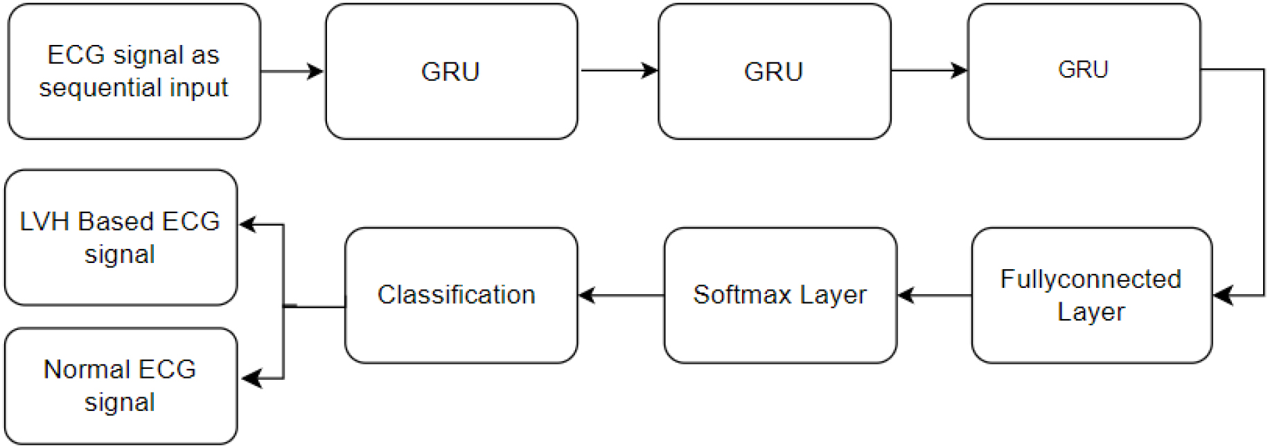

GRU is an enhanced iteration of LSTM that exhibits a swifter training process. It offers a simpler architecture compared to LSTM, featuring reduced computational complexity. The internal flow of unit information is cooperatively regulated by the gates that make up GRU. Notably, the input and forget gates are consolidated to create a unique gating element known as the update gate. The primary function of the update gate is to meticulously manage the state equilibrium between the preceding and the candidate activation [41].

4.7 GRU architecture

A GRU is regarded as a simplified version of the LSTM that has two gates, namely the update ( $z_{t}$ ) and the Reset gate ( $R_{t}$ ), and regulates the flow of information. GRU performance has been found to be comparable to LSTM performance even with these simplifications [41]. GRU’s architecture is shown in Fig. 10.

Figure 10.

GRU architecture [41].

Furthermore, GRU can lower the quantity of calculations needed for each training session. Equations (10–(13) can be used to express these computations [41]:

$\displaystyle Z_{t}=W^{xz}x_{t}+W^{hz}H_{t-1}+b_{z}$ (10) $\displaystyle{R}_{t}={W}^{{xr}}{x}_{t}+{W}^{{hr}}{H}_{{t}-1}+{b}_{r}$ (11) $\displaystyle\widetilde{H_{t}}=\text{tanh}({Wx_{t}+WH_{t-1}rR_{t}})$ (12) $\displaystyle H_{t}=(1-z_{t}).H_{t-1}+z_{t}.\widetilde{H_{t}}$ (13)

5. Results and discussion

To evaluate the efficacy of our suggested methodology numerous experiments were carried out. The ECG signal data have been grouped for the evaluation of the model including 80% for training, and 20% for testing and validation. The various LSTM models were implemented to assess their performance in classifying LVH data from an ECG dataset. A one-dimensional CNN network with LSTM models can be employed for analyzing ECG data, as the ECG signal is inherently one-dimensional. The first model is a Conv2LSTM Model. Furthermore, various models including Dual-LSTM Model, Double-Bilayer LSTM model, and GRU3Net Model were implemented.

5.1 Analysis of Conv2LSTM model for the LVH classification

The primary objective was to investigate the influence of deepening networks of CNN on the available dataset. Notably, filter numbers were progressively elevated to 32, 64, 128, and 256, with corresponding kernel sizes of 5, 3, 5, and 10, respectively. While networks of CNN are predominantly employed for end-to-end classification, the layers of intermediates of these models yield feature maps that encapsulate abundant and valuable information.

For the experimental investigation, the CNN networks were individually employed on LVH data. While the data was analyzed, no notable distinctions emerged in the performances of CNN during the training phase. The Conv2LSTM model is developed using batch sizes of 10 and trained over 50 epochs. The Adam’s algorithm for optimization with a learning rate of 0.001 was utilized. To enhance generalization, employing a dropout rate of 0.7. Convolution layers did not introduce bias, and to address the class imbalance, weighted loss was implemented. The max pooling was consistently applied after the convolution layers, facilitating the extraction of optimal features for classification. To determine the efficacy of the model, ten-fold cross-validation is employed. This involved partitioning the data into training the model on 80% of the data, and testing and validating the remaining 20%. Feature extraction from input signals was achieved through the application of convolutional layers, generating feature maps that served as inputs for subsequent layers. Following each convolutional layer, max-pooling layers were incorporated to highlight key features. To improve the model’s ability to generalize and prevent overfitting, dropout layers were strategically introduced in the architecture.

The feature maps clearly shown in Fig. 11 indicate that The model can pick up on pertinent features that can be extracted from the data, even in the presence of noise. Even at a low noise level, the feature maps show clear peaks at the locations of the underlying signal. This suggests that the model can identify the signal and isolate it from the noise. As the noise level increases, the feature maps become more noisy, but the model is still able to learn to extract relevant features. This is evident from the fact that the feature maps still show peaks at the locations of the underlying signal, even at a high noise level. Overall, the feature maps provide strong evidence that the convolution 1D layer can learn effective representations of the time series data, even in the presence of noise.

Figure 11.

Feature maps of convolution layer with the various filter size and number of filters (a) 10 and 250 (b) 10 and 256 (c) 5 and 32 (d) 3 and 64.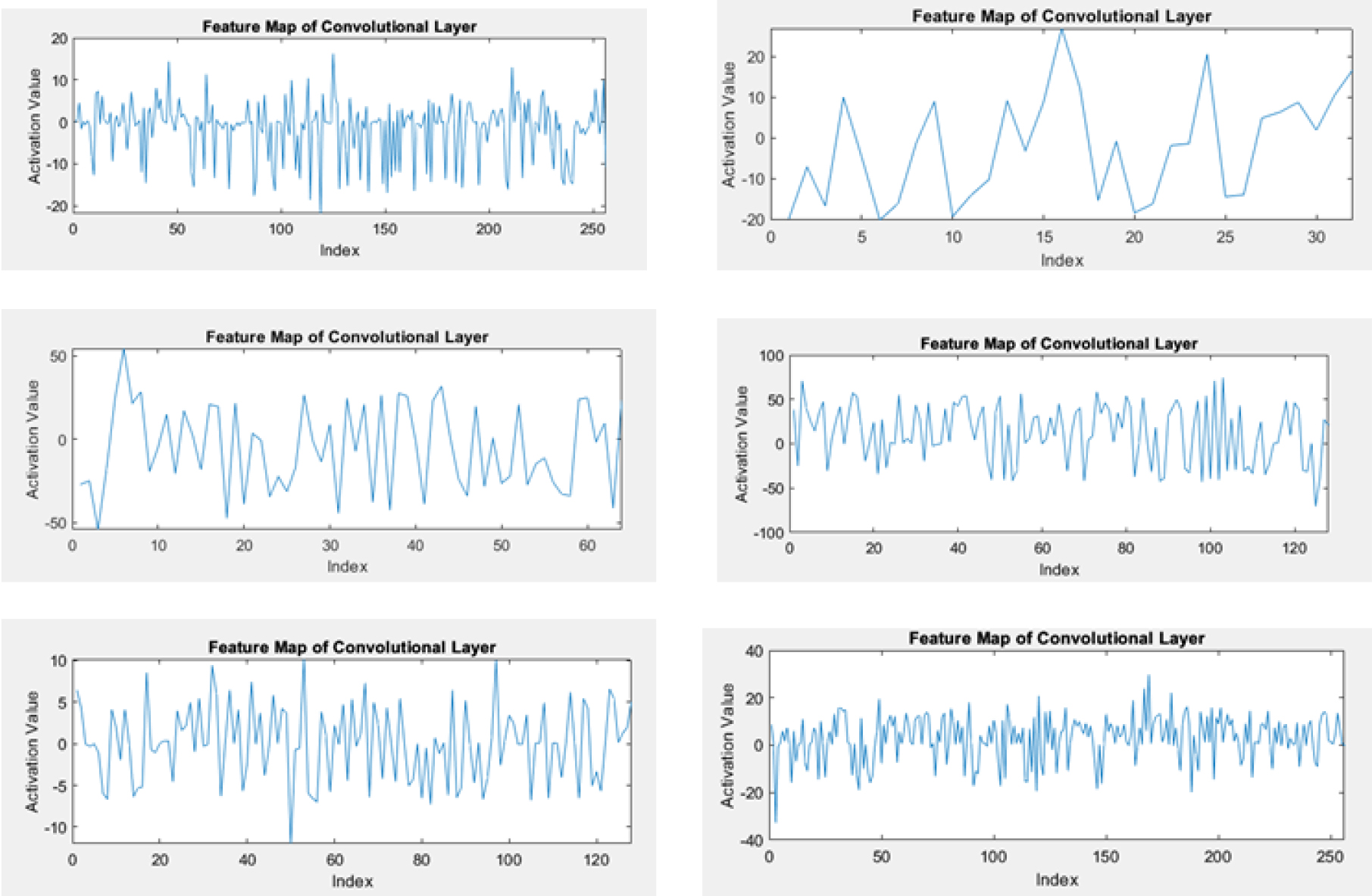

The analysis of the Convolution 1D with LSTM layer results reveals that, overall, increasing the kernel size enhances accuracy, reaching its peak at a size of 10. This implies that capturing broader temporal dependencies within the data contributes positively to the task. However, the observed improvement diminishes when the kernel size reaches 25, hinting at a potential overfitting issue associated with larger kernels. The general, increasing the number of filters improves accuracy up to a certain threshold. The model achieves its highest accuracy when employing 250 filters, emphasizing the benefit of learning diverse features. Nevertheless, a slight decline in performance is observed when using 500 filters, hinting at the possibility of redundancy and overfitting with a higher number of filters. Table 1 presents the comprehensive results obtained from the Conv2LSTM model, showcasing its performance in the classification of LVH.

Table 1

Results obtained from the Conv2LSTM model

Kernel size	No. of filters	Strides	Sensitivity	Specificity	Precision	F1 score	Accuracy
5	128	3	97.7	74.3	78.7	87.2	85.8
12	250	5	84.4	85.4	84.9	84.7	84.7
10	250	3	96.7	77.8	81.4	88.4	87.3
10	500	3	93.4	74.8	78.6	85.4	84.1
25	256	5	76.1	90.8	89.3	82.1	83.4
16	256	5	79.6	88.5	87.1	83.2	84.1
36	256	3	96.0	73.5	78.7	86.5	84.9
36	512	3	76.3	91.5	89.8	82.4	84.6
45	512	3	96.4	77.1	81.2	88.2	86.9
3	96	3	76.0	92.2	90.7	82.7	84.1

The examination of the impact of strides reveals that configurations with strides set at 3 consistently outperform those with strides of 5. This consistency suggests the significance of capturing more fine-grained temporal information, emphasizing the model’s benefit from analyzing data points in closer proximity. When evaluating the overall performance, the best configuration attains an accuracy of 0.893, underscoring the effectiveness of Convolution 1D with the LSTM layer for time series data. Specifically, the combination of a kernel size of 10, 250 filters, and strides of 3 emerges as optimal, showcasing its proficiency in extracting and learning temporal dependencies. The highest sensitivity 97.7% is observed with a kernel size of 5 and 128 filters, highlighting its ability to identify positive instances effectively. Specificity ranges from 73.5% to 92.2%, demonstrating the models’ ability to identify true negative cases. Higher specificity is achieved with larger kernel sizes and fewer filters, suggesting a balance between sensitivity and specificity.

The configuration with a kernel size of 5, 128 filters, and strides of 3 appears to be the most sensitive, while the configuration with a kernel size of 36, 512 filters, and strides of 3 offers the highest specificity. The observed accuracies can be attributed to the effective utilization of LSTM layers in capturing intricate temporal dependencies within sequential ECG data. Additionally, the initial feature extraction capability of the convolutional layer contributed significantly to the model’s ability to discern relevant patterns indicative of Left Ventricular Hypertrophy (LVH). Increasing the number of filters generally leads to higher sensitivity and precision but may also decrease specificity. Larger kernel sizes often result in higher specificity but lower sensitivity. The optimal configuration depends on the specific application and the relative importance of sensitivity, specificity, and overall accuracy.

5.2 Analysis of Dual-LSTM model for the LVH classification

The Dual LSTM model is a deep learning architecture that combines two LSTM networks to address delicate sequential tasks. Figure 12 depicts the relationship between accuracy and loss for Dual-LSTM models with various hidden units: 512, 256, 225, 150, 75, and 64. Hidden units are a crucial parameter in recurrent neural networks (RNNs) like Dual-LSTMs, influencing the model’s capacity to learn delicate patterns from sequential inputs.

Figure 12.

Accuracy and loss of Dual-LSTM models with the various hidden units including 512, 256, 225,150, 75, 64.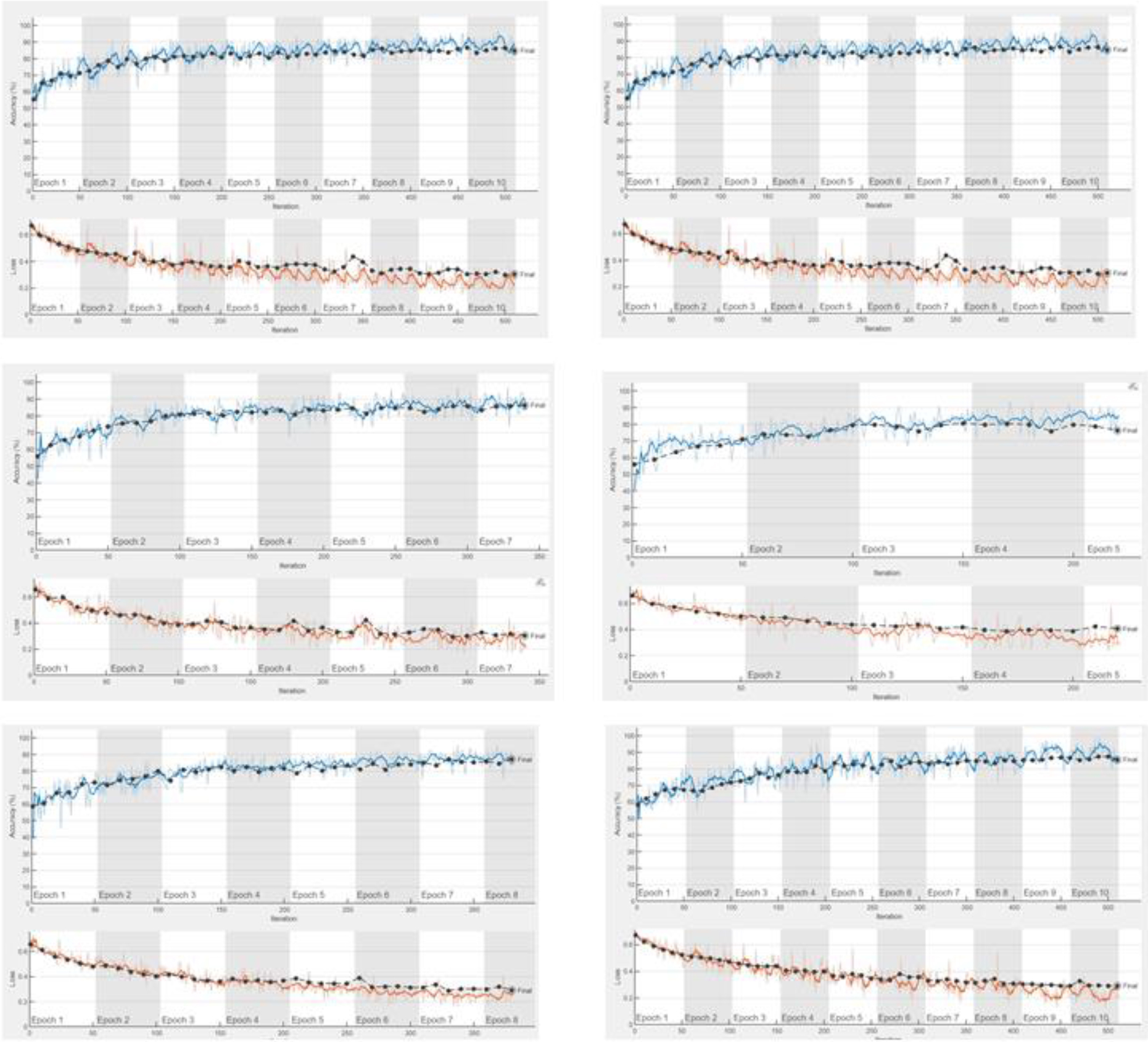

The initial loss of approximately 0.7 steadily decreases to around 0.2 by the conclusion of the training, while the accuracy climbs from around 0.6 at the outset to approximately 0.9 by the training’s end. These outcomes signify the LSTM layer’s aptitude for learning long-term dependencies within the data, resulting in accurate predictions. Moreover, the model exhibits robust generalization to unseen data, as evidenced by the similarity between validation and training accuracy.

The overall training progress is highly promising, suggesting the model’s suitability for the time series forecasting task. Additional observations note the smooth and stable nature of the loss and accuracy curves, indicating a consistent and stable learning process. A slight overshoot in accuracy around epoch 100 is swiftly stabilized, implying a well-fitted model without overfitting. Although the validation accuracy consistently lags slightly behind the training accuracy, the marginal difference underscores the model’s commendable capacity to predict effectively to new data effectively. In summary, the training progress strongly indicates that the LSTM layer adeptly learns to make accurate predictions for the time series forecasting task. Table 2 displays the results attained through the Dual-LSTM model, highlighting the performance metrics and outcomes achieved in the classification of Left Ventricular Hypertrophy (LVH).

Table 2

Results obtained from the Dual-LSTM model

Number of hidden layers	Learn rate drop period	Learn rate drop factor	Validation frequency	Sensitivity	Specificity	Precisions	F1 score	Accuracy
256	10	0.7	10	69.4	94.5	92.6	79.4	79.3
256	10	0.8	10	96.8	73.1	78.2	86.5	86.3
225	10	0.8	10	98.4	80.5	83.4	90.3	90.8
150	10	0.8	10	81.5	95.8	95.2	87.8	87.8
75	10	0.8	10	96.2	78.8	82.1	88.6	88.8
256	8	0.3	8	97.5	74.8	79.8	87.7	87.6
256	8	0.3	10	92.5	83.8	85.2	88.7	88.3
225	8	0.3	10	95.8	79.1	82.2	88.5	88.7
64	8	0.3	10	86.15	91.4	90.8	88.4	88.6
512	8	0.3	10	98.7	75.5	80.2	88.5	88.8

Raising the number of hidden units generally improves the model’s performance, with 512 hidden layer configurations achieving the highest accuracy of 90.8%. However, this comes at the cost of computational complexity. There seems to be no consistent trend with varying the learning rate drop period. While longer periods of 10 tend to perform better for some configurations, others benefit from shorter periods of 8. Increasing the learning rate drop factor to 0.8 generally leads to higher accuracy compared to factors 0.7 and 0.3. This suggests a faster decrease in the learning rate might be beneficial. Increasing the validation frequency to 10 seems to result in better performance compared to lower frequencies 8. This indicates more frequent evaluation helps the model generalize better.

The table provides valuable insights into the performance of the machine learning model under different configurations. It highlights the balance between complexity, accuracy, and other performance of the model. Based on this analysis, the 225 hidden layer configuration with a learning rate drop factor of 0.8 and validation frequency of 10 appears to be the optimal choice, achieving high accuracy while maintaining reasonable complexity. Analyzing the model’s training process, such as loss curves, could provide further insights into the learning dynamics and potential areas for improvement. The lower accuracy of 90.8% for the bilayer LSTM could be attributed to its complex structure, which involves more parameters and can lead to overfitting.

5.3 Double-Bilayer LSTM model

The count of epochs set for learning the bilayer LSTM model is 100 epochs. The minimum batch size utilized during training, influencing the number of samples processed in each iteration is 64. The frequency at which model performance is assessed on the validation set during training is 10 epochs. The learning rate used during training determines the step size for weight updates. The table presents the results obtained from the proposed Double-Bilayer LSTM Model, elucidating the performance metrics and outcomes in the Classification of LVH signal from normal ECG signal.

Table 3
Results obtained from the proposed Double-Bilayer LSTM model

Number of hidden layers	Sensitivity	Specificity	Precisions	F1 score	Accuracy
220	91.2	91.2	91.2	91.2	87.9
225	95.2	90.6	91.1	93.1	89.5
256	95.1	97.3	97.3	96.2	91.7
125	98.0	94.1	94.4	96.1	90.4
100	99.3	80.2	83.2	90.2	83.8
64	99	93.8	94.2	96.5	91.5
32	91.0	88.4	89.7	89.7	83.7

In the above table, sensitivity significantly improves with hidden layers, peaking at 98.0% with 225 layers, showcasing enhanced positive case identification. The specificity generally decreases with more hidden layers, reaching its highest value of 97.3% at 256 layers, striking a balance between sensitivity and specificity. The precision follows a similar trend as sensitivity, achieving a peak of 97.3% with 256 layers, indicating accurate identification of true positives among predicted positives. F1 Score peaks at 96.5% with 64 hidden layers, demonstrating balanced performance of the sensitivity and specificity. The accuracy peaks at 91.7% with 256 hidden layers, indicating optimal overall model performance. However, there is a general decrease as sensitivity prioritizes positive cases over specificity. The model with 256 hidden layers attains the best overall performance, effectively balancing sensitivity, specificity, and accuracy. Higher hidden layers prioritize sensitivity, potentially sacrificing specificity, while lower layers prioritize specificity at the expense of sensitivity. Double-bilayer LSTM tends to have lower accuracy compared to GRU3Net because GRU3Net’s streamlined gating mechanism results in fewer parameters, helping to reduce overfitting and improve generalization.

5.4 GRU3Net model

The GRU3Net model was learned for 50 epochs, employing a minimum size of batch 64, which dictates the number of samples processed in each iteration. The validation set’s performance was evaluated at intervals of 10 epochs during the training process. Additionally, the learning rate, a crucial parameter governing the step size for weight updates, was specified for the training phase. The key feature responsible for the high accuracy of GRU3Net is its advanced temporal feature extraction capability, facilitated by the multiple layers of GRUs. This allows the model to maintain and update hidden states effectively, capturing long-term dependencies and complex patterns in ECG data crucial for accurate LVH detection.

Table 4 presents the results obtained from the GRU3Net Model for the classification of LVH.

Table 4
Results obtained from the proposed GRU3Net model

Number of hidden layers	Sensitivity	Specificity	Precisions	F1 score	Accuracy
200	99.2	92.7	93.4	96.2	96.1
225	98.0	91.7	92.1	95.0	95.3
256	99.2	90.2	91.1	95.0	95.6
125	92.9	96.0	95.8	94.4	94.5
100	99.5	88.0	89.1	94.7	93.6
64	99.6	90.1	95.6	94.8	89.9
32	99.8	90.0	91.6	95.2	94.9

The models under consideration exhibit exceptional sensitivity, consistently surpassing 99%, even with variations in hidden layer configurations such as 256, 200,100, and 32 layers. This indicates a commendable capacity to determine true positive cases accurately. In contrast, specificity demonstrates variability across models, spanning from 88% with 100 hidden layers to 96% with 125 hidden layers. Notably, models with heightened sensitivity tend to display lower specificity, underscoring the inherent trade-off between these two metrics. The precision aligns closely with the sensitivity trend, reaching 95.6 with 64 and 256 hidden layers. This pattern suggests that the models excel in accurately identifying true positives among the instances predicted as positive. The F1 score, providing a balanced perspective on sensitivity and precision, attains its highest value at 96.2 with 200 hidden layers, showcasing overall robust performance. The accuracy peaks at 96.1% with 200 hidden layers, indicating the optimal model configuration for overall accuracy. Notably, accuracy slightly decreases with excessively high or low numbers of hidden layers, suggesting potential overfitting concerns.

Further, refinement and optimization are recommended through additional analysis, considering factors such as model complexity and data imbalance. The results also offer valuable insights into the impact of hidden layer size on various performance metrics, providing a foundation for informed model selection based on efficiency and effectiveness for the given task.

5.5 Comparative analysis

This paper discusses a comparative analysis of various deep-learning models for the automated classification of LVH from electrocardiogram (ECG) signals. LVH is a critical cardiac condition characterized by the enlargement of the left ventricle, leading to potential heart failure and other complications. Comparing the performance of this model with other models on the same task would allow for a more comprehensive evaluation of its effectiveness. The tuning parameters of various models are given in the Table 5.

Table 5
Epochs and batch size for various models to detect LVH

Models	Epochs	Batch size
Conv2LSTM	50	10
Double Bilayer LSTM	100	64
Dual LSTM	100	64
Double-Bilayer LSTM model	100	64
GRU3Net	50	64

Table 6 offers a comparative analysis between an existing model and the proposed model for the classification of LVH, delineating performance metrics and highlighting the advancements or improvements introduced by the proposed model.

Table 6

Comparative analysis of the existing model with the proposed model

Methods	Sensitivity	Specificity	Accuracy
GRU-ELM model [62]	97.8	98.4	95.7
CNN-LSTM [24]	65	57	61
LSTM [24]	68	57	–
ELVHC [26]	66	78	–
LVH-Net model [27]	–	–	76
ENN [28]	–	–	88
Proposed GRU3Net model	99.2	92.7	96.1
Proposed Dual-LSTM model	98.4	80.5	90.8
Proposed Conv2LSTM model	96.7	77.8	87.3
Proposed DoubleBilayerLSTM model	95.1	97.3	91.7

The proposed GRU3Net model exhibits outstanding performance with an impressive accuracy of 96.1%, sensitivity of 99.2%, and specificity of 92.7%. These values surpass all other mentioned models, demonstrating their effectiveness in automated LVH classification. The GRU-ELM Model demonstrated commendable performance by achieving high sensitivity and specificity; however, its overall accuracy of 95.7% falls short when compared to the superior accuracy of GRU3Net. The GRU3Net outperforms with higher accuracy, showcasing its effectiveness in accurately classifying LVH cases. On the other hand, the Conv2LSTM model exhibits challenges with relatively low sensitivity (65%) and specificity (57%), indicating potential difficulties in accurately detecting LVH and distinguishing it from normal cases. Similarly, the standard LSTM model shares these weaknesses in sensitivity (68%) and specificity (57%), highlighting limitations in its ability to effectively discern LVH signals. The ELVHC model, while achieving reasonable specificity at 78%, displays low sensitivity (66%), raising concerns about the potential for missed LVH cases. In the case of LVH-Net, while lacking specific sensitivity and specificity values, its accuracy of 76% suggests a promising foundation for further improvement. The ENN model, akin to LVH-Net, lacks sensitivity and specificity values but achieves a moderate accuracy of 88%. Additionally, the proposed Dual-LSTM Model and Conv2LSTM Model also demonstrate noteworthy performance, achieving high accuracy levels of 90.8% and 87.3%, respectively. The DoubleBilayer LSTM model, although exhibiting high specificity at 97.3%, slightly compromises sensitivity at 95.1% compared to the top-performing GRU3Net.

6. Conclusion

This study introduces an LVH classifier utilizing 1-D CNNs, where the model processes one-dimensional signals and produces classification outcomes. The employment of 1-D CNNs enhances the efficiency of automatic feature extraction through adaptive filters. In contrast to LVH detection systems grounded in traditional machine learning approaches, the proposed model eliminates the dependency on specific features for achieving classification results. The results demonstrate a performance advantage over four comparison methods found in recent literature across three key performance metrics. These findings underscore the efficacy of CNNs in addressing local features.

In this research, the signals derived from ECG signals with LVH manifest as continuous and sequential time series signals, inherently constituting local features. The adeptness of 1-D CNN lies in its ability to precisely capture the distinctive characteristics embedded within these local signals. The proposed GRU3Net model demonstrated superior performance, achieving an accuracy of 96.1%, sensitivity of 99.2%, and specificity of 92.7%. This highlights the potential of GRU-based deep learning architectures for LVH classification. The outcomes further indicate that the suggested automatic classification method holds promise for deployment in the detection of LVH diseases, presenting a potential avenue for streamlining medical processes and alleviating the workload for healthcare professionals.

References

World Health Organization. World health statistics 2018: monitoring health for the SDGs, sustainable development goals [Internet]. www.who.int. 2018.

Baral

Maskey

Malla

Rajbhandari

Adhikari

Bhandari

Shrestha

Pandey

Shimkhada

Budhathoki

. Evaluation of left ventricular systolic function by myocardial deformation imaging in hypertensive patients with preserved left ventricular ejection fraction. Nepalese Heart Journal. 2021 Nov 23; 18(2): 15-9.

Rovner

de las Fuentes

Waggoner

Memon

Chohan

Dávila-Román

. Characterization of left ventricular diastolic function in hypertension by use of Doppler tissue imaging and color M-mode techniques. Journal of the American Society of Echocardiography. 2006 Jul 1; 19(7): 872-9.

Sinha

Azukaitis

Sladowska-Kozłowska

Bårdsen

Merkevicius

Karlsen Sletten

Obrycki

Pac

Fernández-Aranda

Bjelakovic

Jankauskiene

. Prevalence of left ventricular hypertrophy in children and young people with primary hypertension: Meta-analysis and meta-regression. Frontiers in Cardiovascular Medicine. 2022 Oct 31; 9: 993513.

Lorell

Carabello

. Left ventricular hypertrophy: Pathogenesis, detection, and prognosis. Circulation. 2000 Jul 25; 102(4): 470-9.

Naimov

. Left ventricular hypertrophy: Diagnosis in 40–60-year-old women with hypertension. European Journal of Interdisciplinary Research and Development. 2022 Jun 30; 4: 186-8.

Miao

Wen

Fortino

Wang

Liu

Tang

. Continuous blood pressure measurement from one-channel electrocardiogram signal using deep-learning techniques. Artificial Intelligence in Medicine. 2020 Aug 1; 108: 101919.

Bornstein

Rao

Marwaha

. Left ventricular hypertrophy. 2020.

Cuspidi

Sala

Negri

Mancia

Morganti

. Prevalence of left-ventricular hypertrophy in hypertension: An updated review of echocardiographic studies. Journal of Human Hypertension. 2012 Jun; 26(6): 343-9.

10.

Marketou

Parthenakis

Vardas

. Pathological left ventricular hypertrophy and stem cells: Current evidence and new perspectives. Stem Cells International. 2016; 2016(1): 5720758.

11.

Pewsner

Jüni

Egger

Battaglia

Sundström

Bachmann

. Accuracy of electrocardiography in diagnosis of left ventricular hypertrophy in arterial hypertension: Systematic review. Bmj. 2007 Oct 4; 335(7622): 711.

12.

Bacharova

. Missing link between molecular aspects of ventricular arrhythmias and QRS complex morphology in left ventricular hypertrophy. International Journal of Molecular Sciences. 2019 Dec 19; 21(1): 48.

13.

Levy

Anderson

Savage

Balkus

Kannel

Castelli

. Risk of ventricular arrhythmias in left ventricular hypertrophy: The Framingham Heart Study. The American Journal of Cardiology. 1987 Sep 1; 60(7): 560-5.

14.

Estes

Zhang

Tereshchenko

Soliman

. Individual components of the Romhilt-Estes left ventricular hypertrophy score differ in their prediction of cardiovascular events: The Atherosclerosis Risk in Communities (ARIC) study. American Heart Journal. 2015 Dec 1; 170(6): 1220-6.

15.

Bacharova

Chen

Estes

Mateasik

Bluemke

Lima

Burke

Soliman

. Determinants of discrepancies in detection and comparison of the prognostic significance of left ventricular hypertrophy by electrocardiogram and cardiac magnetic resonance imaging. The American Journal of Cardiology. 2015 Feb 15; 115(4): 515-22.

16.

Bacharova

Szathmary

Svehlikova

Mateasik

Gyhagen

Tysler

. The effect of conduction velocity slowing in left ventricular midwall on the QRS complex morphology: A simulation study. Journal of Electrocardiology. 2016 Mar 1; 49(2): 164-70.

17.

Moreo

Ambrosio

De Chiara

Tran

Raman

. Influence of midwall fibrosis on diastolic dysfunction in non-ischemic cardiomyopathy. International Journal of Cardiology. 2013 Mar 3; 163(3): 342.

18.

Dweck

Joshi

Murigu

Alpendurada

Jabbour

Melina

Banya

Gulati

Roussin

Raza

Prasad

. Midwall fibrosis is an independent predictor of mortality in patients with aortic stenosis. Journal of the American College of Cardiology. 2011 Sep 13; 58(12): 1271-9.

19.

Leyva

Taylor

Foley

Umar

Mulligan

Patel

Stegemann

Haddad

Smith

Prasad

. Left ventricular midwall fibrosis as a predictor of mortality and morbidity after cardiac resynchronization therapy in patients with nonischemic cardiomyopathy. Journal of the American College of Cardiology. 2012 Oct 23; 60(17): 1659-67.

20.

Shashikumar

Shah

Clifford

Nemati

. A deep learning approach to monitoring and detecting atrial fibrillation using wearable technology. In 2017 IEEE EMBS International Conference on Biomedical & Health Informatics (BHI). IEEE. 2017 Feb 16. pp. 141-144.

21.

Zhou

Yan

Qin

Yuan

Que

Wang

. Deep learning-based classification of massive electrocardiography data. In 2016 IEEE Advanced Information Management, Communicates, Electronic and Automation Control Conference (IMCEC). IEEE. 2016 Oct 3. pp. 780-785.

22.

Jun

Park

Minh

Kim

. Premature ventricular contraction beat detection with deep neural networks. In 2016 15th IEEE International Conference on Machine Learning and Applications (ICMLA). IEEE. 2016 Dec 18. pp. 859-864.

23.

Hasan

Bhattacharjee

. Deep learning approach to cardiovascular disease classification employing modified ECG signal from empirical mode decomposition. Biomedical Signal Processing and Control. 2019 Jul 1; 52: 128-40.

24.

Zhao

Huang

Wang

Zhou

Liu

Lin

Liu

. Deep learning assessment of left ventricular hypertrophy based on electrocardiogram. Frontiers in Cardiovascular Medicine. 2022 Aug 11; 9: 952089.

25.

Khurshid

Friedman

Pirruccello

Di Achille

Diamant

Anderson

Ellinor

Batra

Philippakis

Lubitz

. Deep learning to predict cardiac magnetic resonance-derived left ventricular mass and hypertrophy from 12-lead ECGs. Circulation: Cardiovascular Imaging. 2021 Jun; 14(6): e012281.

26.

Tsai

Xiao

Liaw

. A deep neural network electrocardiogram analysis framework for left ventricular hypertrophy prediction. Journal of Ambient Intelligence and Humanized Computing. 2020 Mar 9; 1-7.

27.

Haimovich

Diamant

Khurshid

Di Achille

Reeder

Friedman

Singh

Spurlock

Ellinor

Philippakis

Batra

. Artificial intelligence-enabled classification of hypertrophic heart diseases using electrocardiograms. Cardiovascular Digital Health Journal. 2023 Apr 1; 4(2): 48-59.

28.

Kwon

Jeon

Kim

Lim

Kim

Song

Park

Choi

. Comparing the performance of artificial intelligence and conventional diagnosis criteria for detecting left ventricular hypertrophy using electrocardiography. EP Europace. 2020 Mar 1; 22(3): 412-9.

29.

Saadatnejad

Oveisi

Hashemi

. LSTM-based ECG classification for continuous monitoring on personal wearable devices. IEEE Journal of Biomedical and Health Informatics. 2019 Apr 14; 24(2): 515-23.

30.

Zhang

Dai

Zhou

Wang

. Interpretability analysis of heartbeat classification based on heartbeat activity’s global sequence features and BiLSTM-attention neural network. IEEE Access. 2019 Aug 7; 7: 109870-83.

31.

Liu

Wang

Zhao

Yuan

Zhang

. Automatic cardiac arrhythmia classification using combination of deep residual network and bidirectional LSTM. IEEE Access. 2019 Jul 29; 7: 102119-35.

32.

Shashikumar

Shah

Clifford

Nemati

. Detection of paroxysmal atrial fibrillation using attention-based bidirectional recurrent neural networks. In Proceedings of the 24th ACM SIGKDD International Conference on Knowledge Discovery & Data Mining. 2018 Jul 19. pp. 715-723.

33.

Ballinger

Hsieh

Singh

Sohoni

Wang

Tison

Marcus

Sanchez

Maguire

Olgin

Pletcher

. DeepHeart: semi-supervised sequence learning for cardiovascular risk prediction. In Proceedings of the AAAI Conference on Artificial Intelligence. Vol. 32, No. 1. 2018 Apr 26.

34.

Hong

Xiao

Sun

. MINA: multilevel knowledge-guided attention for modeling electrocardiography signals. arXiv preprint arXiv:1905.11333. 2019 May 27.

35.

Wang

Guo

. Simultaneous human health monitoring and time-frequency sparse representation using EEG and ECG signals. IEEE Access. 2019 Jun 10; 7: 85985-94.

36.

Goodfellow

Pouget-Abadie

Mirza

Warde-Farley

Ozair

Courville

Bengio

. Generative adversarial nets. Advances in neural information processing systems. 2014; 27.

37.

Wang

Hou

Shao

Yan

. ECG arrhythmias detection using auxiliary classifier generative adversarial network and residual network. Ieee Access. 2019 Jul 24; 7: 100910-22.

38.

Wołk

. Early and remote detection of possible heartbeat problems with convolutional neural networks and multipart interactive training. IEEE Access. 2019 May 27; 7: 145921-7.

39.

Zhu

Liu

Shen

. Electrocardiogram generation with a bidirectional LSTM-CNN generative adversarial network. Scientific Reports. 2019 May 1; 9(1): 6734.

40.

Hong

Zhou

Shang

Xiao

Sun

. Opportunities and challenges of deep learning methods for electrocardiogram data: A systematic review. Computers in Biology and Medicine. 2020 Jul 1; 122: 103801.

41.

Xiong

Stiles

Zhao

. Robust ECG signal classification for detection of atrial fibrillation using a novel neural network. In 2017 Computing in Cardiology (CinC). IEEE. 2017 Sep 24. pp. 1-4.

42.

Swapna

Vinayakumar

Soman

. Diabetes detection using deep learning algorithms. ICT Express. 2018 Dec 1; 4(4): 243-6.

43.

Zaremba

Sutskever

Vinyals

. Recurrent neural network regularization. arXiv preprint arXiv:1409.2329. 2014 Sep 8.

44.

Krizhevsky

Sutskever

Hinton

. Imagenet classification with deep convolutional neural networks. Advances in neural information processing systems. 2012; 25.

45.

Cheng

Sori

Jiang

Khan

Liu

. Recurrent neural network based classification of ECG signal features for obstruction of sleep apnea detection. In 2017 IEEE International Conference on Computational Science and Engineering (CSE) and IEEE International Conference on Embedded and Ubiquitous Computing (EUC). IEEE. Vol. 2. 2017 Jul 21. pp. 199-202.

46.

Erdenebayar

Kim

Park

Joo

Lee

. Deep learning approaches for automatic detection of sleep apnea events from an electrocardiogram. Computer Methods and Programs in Biomedicine. 2019 Oct 1; 180: 105001.

47.

Schuster

Paliwal

. Bidirectional recurrent neural networks. IEEE Transactions on Signal Processing. 1997 Nov; 45(11): 2673-81.

48.

Graves

Schmidhuber

. Framewise phoneme classification with bidirectional LSTM and other neural network architectures. Neural Networks. 2005 Jul 1; 18(5-6): 602-10.

49.

Yildirim

. A novel wavelet sequence based on deep bidirectional LSTM network model for ECG signal classification. Computers in Biology and Medicine. 2018 May 1; 96: 189-202.

50.

Cho

Van Merriënboer

Bahdanau

Bengio

. On the properties of neural machine translation: Encoder-decoder approaches. arXiv preprint arXiv:1409.1259. 2014 Sep 3.

51.

Doersch

. Tutorial on variational autoencoders. arXiv preprint arXiv:1606.05908. 2016 Jun 19.

52.

Goodfellow

Pouget-Abadie

Mirza

Warde-Farley

Ozair

Courville

Bengio

. Generative adversarial nets. Advances in neural information processing systems. 2014; 27.

53.

Hong

Zhou

Shang

Xiao

Sun

. Opportunities and challenges of deep learning methods for electrocardiogram data: A systematic review. Computers in Biology and Medicine. 2020 Jul 1; 122: 103801.

54.

Simonyan

Zisserman

. Very deep convolutional networks for large-scale image recognition. arXiv preprint arXiv:1409. 1556. 2014 Sep 4.

55.

Dahl

Sainath

Hinton

. Improving deep neural networks for LVCSR using rectified linear units and dropout. In 2013 IEEE International Conference on Acoustics, Speech and Signal Processing. IEEE. 2013 May 26. pp. 8609-8613.

56.

Srivastava

Hinton

Krizhevsky

Sutskever

Salakhutdinov

. Dropout: A simple way to prevent neural networks from overfitting. The Journal of Machine Learning Research. 2014 Jan 1; 15(1): 1929-58.

57.

Kingma

. Adam: A method for stochastic optimization. arXiv preprint arXiv:1412.6980. 2014 Dec 22.

58.

Pang

Wang

. Patient-specific ECG classification by deeper CNN from generic to dedicated. Neurocomputing. 2018 Nov 7; 314: 336-46.

59.

Rajpurkar

Hannun

Haghpanahi

Bourn

. Cardiologist-level arrhythmia detection with convolutional neural networks. arXiv preprint arXiv:1707.01836. 2017 Jul 6.

60.

Yıldırım

Pławiak

Tan

Acharya

. Arrhythmia detection using deep convolutional neural network with long duration ECG signals. Computers in Biology and Medicine. 2018 Nov 1; 102: 411-20.

61.

Fujita

Cimr

. Computer aided detection for fibrillations and flutters using deep convolutional neural network. Information Sciences. 2019 Jun 1; 486: 231-9.

62.

Ramaraj

. A novel deep learning based gated recurrent unit with extreme learning machine for electrocardiogram (ECG) signal recognition. Biomedical Signal Processing and Control. 2021 Jul 1; 68: 102779.

63.

Jothiramalingam

Jude

Patan

Ramachandran

Duraisamy

Gandomi

. Machine learning-based left ventricular hypertrophy detection using multi-lead ECG signal. Neural Computing and Applications. 2021 May; 33: 4445-55.

64.

Goldberger

Amaral

Glass

Hausdorff

Ivanov

Mark

Mietus

Moody

Peng

Stanley

. PhysioBank, PhysioToolkit, and PhysioNet: Components of a new research resource for complex physiologic signals. Circulation. 2000 Jun 13; 101(23): e215-20.

Hybrid LSTM models-based detection of left ventricular hypertrophy in electrocardiogram signals

Abstract

Keywords

1. Introduction

1.1 ECG criteria on LVH

1.2 ECG findings in LVH patients

2. Literature survey

3. Dataset

5.1 Analysis of Conv2LSTM model for the LVH classification

Table 3 Results obtained from the proposed Double-Bilayer LSTM model

Table 4 Results obtained from the proposed GRU3Net model

Table 5 Epochs and batch size for various models to detect LVH

References

Table 3
Results obtained from the proposed Double-Bilayer LSTM model

Table 4
Results obtained from the proposed GRU3Net model

Table 5
Epochs and batch size for various models to detect LVH