A cross-selection instance algorithm

Abstract

Motivated by the idea of cross-validation, a novel instance selection algorithm is proposed in this paper. The novelties of the proposed algorithm are that (1) it cross selects the important instances from the original data set with a committee, (2) it can deal with the problem of selecting instance from large data sets. We experimentally compared our algorithm with five state-of-the-art approaches which are CNN, ENN, RNN, MCS, and ICF on 3 artificial data sets and 6 UCI data sets, including 4 large data sets, ranking from 130K to 4898K in size. The experimental results show that the proposed algorithm is very efficient and effective, especially on large data sets.

Keywords

Instances selection extreme learning machine K–L divergence large data sets

1 Introduction

Instance selection also named sample selection is to select a small representative subset from original data set by removing the redundancy instances. In the framework of classification, the purpose of instance selection is to reduce computational complexity of classification algorithm without degenerating its classification accuracy. Since Hart’s seminal work (i.e. CNN) [1], many instance selection algorithms have been proposed by different researchers. CNN attempts to find a minimal consistent subset (MCS) of the training set. A consistent subset S of a training set T correctly classifies every instance in T with the same accuracy as T itself [2]. CNN algorithm can ensure that all instances in T are classified correctly by S. However, it does not guarantee that S is a MCS. In addition, CNN is especially sensitive to noise, because noisy instances will usually be misclassified by their neighbors, and thus will be retained [3]. The reduced nearest neighbor (RNN) rule proposed by Gates [4] starts with S = T and removes each instance from S if such a removal does not cause any other instances in T to be misclassified by the instances remaining in S. RNN is computationally more expensive than CNN. The selective nearest neighbor rule (SNN) proposed by Ritter [5] improves CNN and RNN by ensuring that a MCS can be found. SNN is much more complex and the computational time is significantly greater than CNN and RNN. Based on the relative significance of the instances in the training set, Dasarathy proposed an algorithm which can identify MCS [6]. The editing nearest neighbor (ENN) rule proposed by Wilson [3] employs the so called editing rule to remove noisy instances in the training set. The rule is that all instances which are incorrectly classified by their nearest neighbors are assumed to be noisy instances. Based on the concepts of coverage and reach ability, the iterative case filtering (ICF) algorithm was introduced in [2]. The reachable set depends on the distance of an instance from its nearest enemy, and the coverage set of every instance is the list of its associates.

Recently, some new instance selection algorithms were developed by different authors. Nikolaidis et al. proposed a class boundary preserving algorithm [7], which discards center instances while it retains a suitable number of border patterns. Based on the concept of Voronoi cells and enemies, Angiulli proposed a fast nearest neighbor condensation (FCNN) algorithm [8] for large data sets classification. The author claimed that FCNN is order independent, its worst-case time complexity is quadratic, and it is likely to select points very close to the decision boundary. Based on the idea of so-called chain which is a sequence of nearest neighbors from alternating classes, Fayed et al. presented a template reduction algorithm [9], the authors make the point that patterns further down the chain are close to the classification boundary. Li presented a critical pattern selection algorithm by considering local geometrical and statistical information [10]. This algorithm selects both border and edge patterns from the data set.

Most of the instance selection algorithms are tailored for nearest neighbor classifier, so the instances selected with these algorithms are often only suitable for nearest neighbor classifiers. In addition, the computational complexities of these algorithms are also very high, for large data sets some algorithms are impracticable. In order to deal with this problem, motivated by the idea of cross validation, we propose a novel instance selection algorithm, which cross selects the important instances from the original data set with a committee. For large data sets, considering the learning efficiency, we use the single-hidden-layer feed-forward neural networks (SLFNs) trained with extreme leaning machine (ELM) [11] as classifiers in the proposed algorithm. ELM has very fast learning speed and very good generalization ability, and it has been successfully applied in function approximation [12, 13], pattern recognition [14, 15], big data classification [16 –18], two comprehensive survey on ELM can be found in [19, 20].

The paper is organized as follows. Some related notions and theoretical background are given in Section 2. The proposed methods are presented in Section 3. Experimental results and analysis are presented in Section 4. Section 5 concludes the paper.

2 Preliminaries

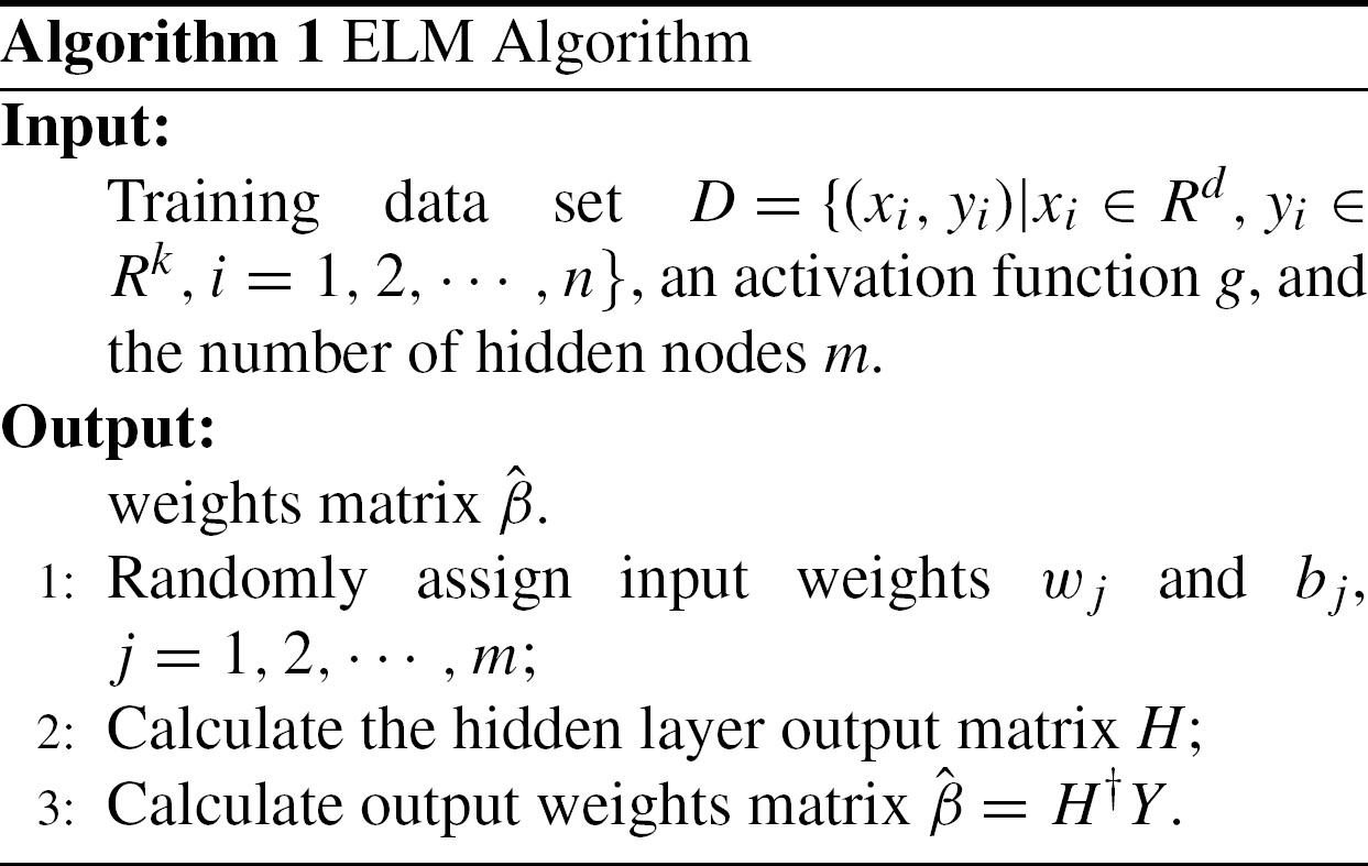
ELM is an efficient and practical learning algorithm used for training the single-hidden-layer feed-forward neural networks (SLFNs) [11]. In ELM the input weights and the hidden layer biases can be chosen randomly, the output weights can be analytically determined with Moore-Penrose generalized inverse [21] of the hidden layeroutput matrix. Unlike other gradient-descent based learning algorithms (such as Back Propagation algorithm [22 –24]), ELM does not require iterative techniques to adjust input weights and hidden layer biases during training process. ELM can overcome many drawbacks of the traditional gradient-based learning algorithms such as local minimal, low learning speed by randomly selecting input weights and hidden layer bias [19, 20].

Given a training data set, D = {(x_i, y_i) |x_i ∈ R^d, y_i ∈ R^k, i = 1, 2, ⋯ , n}, where x_i is a d × 1 input vector and y_i is a k × 1 target vector, a SLFN with m hidden nodes is formulated as $f (x_{i}) = \sum_{j = 1}^{m} β_{j} g (w_{j} \cdot x_{i} + b_{j}), i = 1, 2, \dots, n$ (1)where w_j = (w_j1, w_j2, ⋯ , w_jd) ^T is the weight vector connecting the jth hidden node with the input nodes. b_j is the threshold of the jth hidden node. w_j and b_j are randomly assigned. β_j = (β_j1, β_j2, ⋯ , β_jm) ^T is the weight vector connecting the jth hidden node with the output nodes. The parameters β_j (j = 1, 2, ⋯ , m) may be estimated by least-square fitting with the given training data set D, i.e., satisfying $f (x_{i}) = \sum_{j = 1}^{m} β_{j} g (w_{j} \cdot x_{i} + b_{j}) = y_{i}$ (2) Equation (2) can be written in a more compact format as $H β = Y$ (3)where $H = [\begin{matrix} g (w_{1} \cdot x_{1} + b_{1}) & \dots & g (w_{m} \cdot x_{1} + b_{m}) \\ ⋮ & ⋱ & ⋮ \\ g (w_{1} \cdot x_{n} + b_{1}) & \dots & g (w_{m} \cdot x_{n} + b_{m}) \end{matrix}]$ (4) $β = (β_{1}^{T}, \dots, β_{m}^{T})$ (5)and $Y = (y_{1}^{T}, \dots, y_{n}^{T})$ (6)H is the hidden layer output matrix of the network, where the jth column of H is the jth hidden nodes output vector with respect to inputs x₁, x₂, ⋯ , x_n, and the ith row of H is the output vector of the hidden layer with respect to input x_i. If the number of hidden nodes is equal to the number of distinct training samples, the matrix H is square and invertible, and SLFNs can approximate these training samples with zero error. But generally, the number of hidden nodes is much less than the number of training samples. Therefore, H is a non-square matrix and one cannot expect an exact solution of the system (3). Fortunately, it has been proved in [26] that SLFNs with random hidden nodes have the universal approximation capability and the hidden nodes could be randomly generated. The least-square fitting is to solve the following equation. $min_{β} = ∥ H β - Y ∥$ (7)The smallest norm least-squares solution of (7) may be easily obtained: $\hat{β} = H^{†} Y$ (8)where H^† is the Moore-Penrose generalized inverse of matrix H.

The ELM Algorithm [11] is presented as follows.

For the trained SLFN, the outputs are transformed into the interval (0, 1) with softmax function [22], the transformed results can be viewed as posterior probability p (w_k|x_i), where w_k is the kth class, and x_i is the ith input vector. The p (w_k|x_i) is calculated as: $p (w_{k} | x_{i}) = \frac{e^{y_{ij}}}{\sum_{j = 1}^{k} e^{y_{ij}}}$ (9)

3 Cross-selection instance algorithm

In this section, we first present the idea of the proposed algorithm, and then present the proposed algorithm.

3.1 The idea of the proposed algorithm

The idea of the proposed algorithm is illustrated as Fig. 1. We firstly partition the data set into n disjoint subsets, for each subset S_i (i = 1, 2, ⋯ , n), we use a committee B to select the important instances from S_i. The committee B consists of n - 1 SLFNs which are trained on other n - 1 subsets. Fig. 2 shows an example of the algorithm for 1 round, the data set used in this example includes 50 instances.

The K-L divergence [26] is employed to measure the significance of the samples, the K-L divergence also called relative entropy is a measure of distance between two distributions [26]. Let x be a discrete random variable, p (x) and q (x) are its two probability mass functions, the definition of K-L divergence is given as follows [26]. $D (p | q) = \sum_{x \in V} p (x) log \frac{p (x)}{q (x)}$ (10)In the above definition, we let $0 {log}_{2} \frac{0}{0} = 0$ , $0 {log}_{2} \frac{0}{q} = 0$ and $p {log}_{2} \frac{p}{0} = \infty$ .

Let SLFN₁, SLFN₂, ⋯, SLFN_n are the members of the committee B. The informative instances are selected with the following criteria. $x^{*} = arg max_{x} {avg (D (P_{{SLFN}_{i}} | P_{B}))}$ (11)where $avg (D (P_{{SLFN}_{i}} | P_{B})) = \frac{1}{n} \sum_{i = 1}^{n} D (P_{{SLFN}_{i}} | P_{B})$ (12) $\begin{matrix} D (P_{SLFN i} | P_{B}) \\ = \sum_{k = 1}^{k} P_{{SLFN}_{i}} (w_{k} | x) {log}_{2} \frac{P_{{SLFN}_{i}} (w_{k} | x)}{P_{B} (w_{k} | x)} \end{matrix}$ (13) $P_{B} (w_{k} | x) = \frac{1}{n} \sum_{i = 1}^{n} P_{{SLFN}_{i}} (w_{k} | x)$ (14)

3.2 The cross-selection instance algorithm

The proposed algorithm named ELM-KL is described as follows.

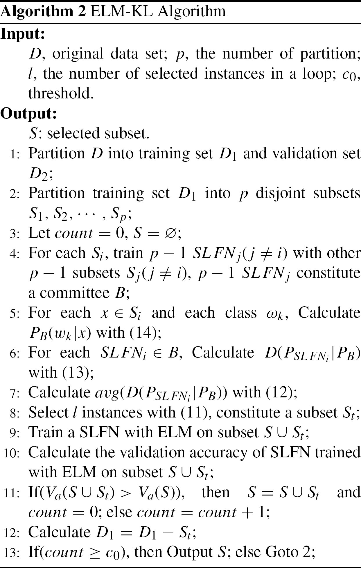
In the ELM-KL algorithm, V_a (S) denotes the validation accuracy of a classifier which is trained on data set S. We also developed another instance selection algorithm named ELM-KL-ALL, which is similar to ELM-KL, the only difference is that ELM-KL-ALL does not introduce validation set, the trained ELM classifier are validated on training set itself.

4 Experiments and the analysis of the experimental results

4.1 Experiments settings and the experimental results

The effectiveness of our proposed method is verified through numerical experiments in the environment of Matlab 7.0 on a Pentium 4 PC. In our experiments we totally select 3 artificial data sets and 6 UCI data sets [27]. The 3 artificial data sets are mainly used to verify the feasibility of the proposed algorithm. The 6 UCI data sets are used to verify the effectiveness and efficiency of the proposed algorithm, we select data sets letter and shuttle because that they contain many categories, the number of classes of the two data sets are 27 and 7 respectively, we select data sets MiniBooNE, skin, artificial_2 and cod_rna because that they are large data sets. The basic information of the 6 UCI data sets is listed in Table 1.

The first artificial data set is two-dimensional concentric data with two classes which are uniform concentric circular distributions [28]. The points of the class ω₁ are uniformly distributed into a circle of radius 0.3 centered on (0.5, 0.5). The points of the class ω₂ are uniformly distributed into a ring centered on (0.5, 0.5) with internal and external radii equal to 0.3 and 0.5, respectively.

The second artificial data set is two-dimensional cloud data with two equal priori probable classes [28]. The class ω₁ is the sum of three different Gaussian distributions: $p (x | ω_{1}) = \frac{1}{2} (\frac{p_{1} (x)}{2} + \frac{p_{2} (x)}{2} + p_{3} (x))$ (15)

Where, x = (x₁, x₂), and $\begin{matrix} p_{i} (x) & = \frac{1}{2 π σ_{{ix}_{1}} σ_{{ix}_{2}}} \\ \times exp (- \frac{(x_{1} - μ_{{ix}_{1}})^{2}}{2 σ_{{ix}_{1}}^{2}} - \frac{(x_{2} - μ_{{ix}_{2}})^{2}}{2 σ_{{ix}_{2}}^{2}}) \end{matrix}$ (16)where μ_{ix
₁} and μ_{ix
₂} are the means of the components x₁ and x₂ of the ith distribution, σ_{ix
₁} and σ_{ix
₂} are the corresponding standard deviations.

The class ω₂ is a single Gaussian distribution: $p (x | ω_{2}) = \frac{1}{2 π} exp (- \frac{x_{1}^{2} + x_{2}^{2}}{2})$ (17)

The third artificial data set is a three-dimensional Gaussian data denoted Gaussian with four classes ω_i (i = 1, 2, 3, 4), the distribution of ω_i is p (x|ω_i) ∼ N (μ_i, Σ_i)

Where, $\begin{matrix} μ_{1} = (0, 0, 0), Σ_{1} = [\begin{matrix} 1 & 0 & 0 \\ 0 & 1 & 0 \\ 0 & 0 & 1 \end{matrix}] \\ μ_{2} = (0, 1, 0), Σ_{2} = [\begin{matrix} 1 & 0 & 1 \\ 0 & 2 & 2 \\ 1 & 2 & 5 \end{matrix}] \\ μ_{3} = (- 1, 0, 1), Σ_{3} = [\begin{matrix} 2 & 0 & 0 \\ 0 & 6 & 0 \\ 0 & 0 & 1 \end{matrix}] \\ μ_{4} = (0, 0.5, 1), Σ_{4} = [\begin{matrix} 2 & 0 & 0 \\ 0 & 2 & 0 \\ 0 & 0 & 3 \end{matrix}] \end{matrix}$

The basic information of the 3 artificial data sets is listed in Table 2. In our experiments, the values of the attributes of all the data sets are normalized into [–1, 1]. Two thirds of the instances are used as training set, and one third of the instances are used as testing set.

The performances of the proposed algorithms ELM-KL and ELM-KL-ALL are compared with original ELM (ORI in short) and ELM-NN on 4 aspects: the number of selected instances, the optimal number of hidden nodes of SLFNs, the testing accuracy, and the training time. ELM-NN is another instance selection algorithm proposed in our previous work [29]. The experimental results on 3 artificial data sets are listed in Table 3, the experimental results on 6 UCI data sets are listed in Table 4.

From the experimental results listed in Tables 3 and 4, we can find that although the testing accuracies of the proposed algorithm trained on the selected subset are lower than the ones trained on the whole data set on all ten data sets, the difference of the experimental results are slight, and the requirements of memory space and the training time are much less than the ones needed on the whole data set. In the framework of the competence preservation, the proposed algorithm is very effective and efficient. The numbers of optimal hidden nodes in Tables 3 and 4 are determined by using the method proposed in our previous work [30]. The curves described the relationship between the testing accuracy and the number of hidden nodes on the subsets selected from the 3 artificial data sets, and the 6 UCI data sets with ELM-EN, ELM-KL, ELM-KL-ALL and original ELM (ORI in short) are shown in Fig. 3 and Fig. 4 respectively.

We also compare our algorithm with five state-of-the-art approaches CNN, ENN, RNN, MCS, and ICF. The comparisons of performances on 3 artificial data sets are listed in Tables 5 to 7. The comparisons of performance on the 6 UCI data sets are listed in Tables 8 to 13. where “-” means that the results cannot be obtained. Compared with CNN, ENN, and RNN, our algorithm removes much more instances while obtaining the similar accuracies. Although ICF and MCS have lower selected ratio than our algorithm, they run much slowly than ours. Our algorithm has a compromise between time and selected ratio. What’s more, four classical algorithms ENN, RNN, ICF, MCS do not work out results on the two largest data set selected in our experiments, i.e. artificial_2 and cod_rna. Two classical algorithms MCS and ICF do not work out results on data sets Shuttle and MiniBooNE. RNN does not work out results on artificial data set gaussian. Our proposed algorithms can work well on large data sets.

4.2 The analysis of the experimental results

In this section, we present a theoretical analysis of the computational time complexity of the proposed algorithm ELM-KL to specify the possible reasons of the results of the experiment. The ELM-KL (algorithm 2) consists of 13 steps, it is obviously, the computational complexity of the step 1, 2 and 3 are O (n), O (n) and O (1) respectively. The step 4 of algorithm 2 is actually to train p SLFN with ELM algorithm, it is well known that the main computational cost of ELM comes from the calculation of the Moore-Penrose generalized inverse of hidden layer output matrix H. Huang et al. [11] pointed out that, when the n training samples are distinct, the hidden-layer output matrix H is column full rank with probability one, so the ELM can be solved as a full-rank least-square problem [31]. For such a problem, some methods, such as orthogonal project, Householder triangularization, and Gram-Schmidt orthogonalization, may be used to solve it, with computational time complexity O (m²n) [21]. Hence, the computational time complexity of ELM algorithm is O (m²n), where m is the number of attributes. When m ⪡ n, the computational time complexity of ELM can be thought to approach O (n) [31]. Accordingly, the computational complexity of the step 4 is O (pn). It is easy to find that the computational time complexity of step 5, 6, 7 and 8 are O (n), O (kn), O (p) and O (lp), where k is the number of classes. Obviously, the computational time complexity of step 9, 10, 11, 12 and 13 are O (lp), O (1), O (1), O (1) and O (1) respectively. Hence, the computational time complexity of the proposed algorithm is $O (n) + O (n) + O (1) + O (\frac{n}{p}) + O (n) + O (kn) + O (p) + O (lp) + O (lp) + O (1) + O (1) + O (1) + O (1)$ . Generally, the number of classes k and the number of selected instances in a loop l are far less than the number of instances of training set n, so the computational time complexity of the proposed algorithm is O (pn).

The computational time complexity of CNN, ENN, RNN, MCS, and ICF are O (n²), O (qn²), O (n³), O (n³) and O (qn²) [32], where q is the nearest numbers. For convenient comparison, the computational time complexities of the 6 algorithms are summarized in Table 14.

Based on the above analysis, it can be seen from Table 14 that the computational time complexity of ELM-KL is the minimum among the 6 algorithms. The consequence of theoretical analysis justify the experimental results, for example, it can be seen from Tables 12 and 13 that four classical algorithms ENN, RNN, ICF, MCS do not work out results on the two largest data set selected in our experiments, i.e. artificial_2 and cod_rna. The possible reasons is that the computational time complexity of the four classical algorithms are to high to work out results on large data sets.

5 Conclusions

Motivated by the idea of cross-validation, in this paper, we proposed two instance selection algorithms which are practicable in large data sets, while some classical algorithms (e.g. ENN, RNN, ICF, MCS) are impracticable. Further more, the proposed algorithms have two advantages: fast leaning speed and low selected ratio. The low selected ratio is achieved by discarding the new selected instances which cannot increase the testing accuracy in each loop. The fast leaning speed is due to the choice of extreme learning machine. The experimental results have verified that the proposed algorithms are much more feasible and effective than five state-of-the-art approaches CNN, ENN, RNN, MCS, and ICF. There are two problems related to our work are worth further investigating, the one problem is how to deploy the proposed algorithms to cloud computing environment, such as, Hadoop MapReduce environment? The other problem is how to scale the proposed algorithms to imbalanced data sets? especially imbalanced big data.

Acknowledgments

This research is supported by the national natural science foundation of China (61170040, 71371063), by the natural science foundation of Hebei Province (F2013201110, F2013201220), by the Key Scientific Research Foundation of Education Department of Hebei Province (ZD20131028) and by the Opening Fund of Zhejiang Provincial Top Key Discipline of Computer Science and Technology at Zhejiang Normal University, China.

References

Hart

, The condensed nearest neighbor rule, IEEE Transaction on Information Theory 14(5) (1967), 515–516.

Brighton

and Mellish

, Advances in instance selection for instance-based learning algorithms, Data Mining and Knowledge Discovery 6(2) (2002), 153–172.

Wilson

D.R.

and Martinez

T.R.

, Reduction techniques for instance-based learning algorithms, Machine Learning 38(3) (2000), 257–286.

Gates

G.W.

, The reduced nearest neighbor rule, IEEE Transactions on Information Theory 18(3) (1972), 431–433.

Ritter

G.L.

, Woodruff

H.B.

and Lowry

S.R.

, An algorithm for a selective nearest neighbor decision rule, IEEE Transactions on Information Theory 21(6) (1975), 665–669.

Dasarathy

B.V.

, Minimal consistent set (MCS) identification for optimal nearest neighbor decision systems design, IEEE Transactions on Systems, Man, And Cybernetics 24(1) (1994), 511–517.

Nikolaidis

, Goulermas

J.Y.

and Wu

Q.H.

, A class boundary preserving algorithm for data condensation, Pattern Recognition 44(3) (2011), 704–715.

Angiulli

, Fast nearest neighbor condensation for large data sets classification, IEEE Transactions on Knowledge and Data Engineering 19(11) (2007), 1450–1464.

Fayed

H.A.

and Atiya

A.F.

, A novel template reduction approach for the k-nearest neighbor method, IEEE Transactions on Neural Networks 20(5) (2009), 890–896.

10.

Y.H.

and Maguire

, Selecting critical patterns based on local geometrical and statistical information, IEEE Transactions on Pattern Analysis and Machine Intelligence 33(6) (2011), 1189–1201.

11.

Huang

G.B.

, Zhu

Q.Y.

and Siew

C.K.

, Extreme learning machine: Theory and applications, Neurocomputing 70(1-3) (2006), 489–501.

12.

Huang

G.B.

, Zhou

H.M.

, Ding

X.J.

and Zhang

, Extreme learning machine for regression and multiclass classification, IEEE Transactions on Systems, Man, and Cybernetics, Part B 42(2) (2012), 513–529.

13.

Lan

, Soh

Y.C.

and Huang

G.B.

, Constructive hidden nodes selection of extreme learning machine for regression, Neurocomputing 73 (2010), 3191–3199.

14.

Chacko

B.P.

, Krishnan

V.R.V.

, Raju

and Anto

P.B.

, Handwritten character recognition using wavelet energy and extreme learning machine, International Journal of Machine Learning and Cybernetics 3(2) (2012), 149–161.

15.

, Wang

S.T.

and Chung

F.L.

, Positive and negative fuzzy rule system, extreme learning machine and image classification, International Journal of Machine Learning and Cybernetics 2(4) (2011), 261–271.

16.

Wang

, Huang

, Qiu

, Liu

and Wang

, Parallel online sequential extreme learning machine based on MapReduce, Neurocomputing 149(Part A) (2015), 224–232.

17.

Wang

, He

Y.L.

, Chow

C.Y.

, Ou

F.F.

and Zhang

, Learning ELM-Tree from big data based on uncertainty reduction, Fuzzy Sets and Systems 258 (2015), 79–100.

18.

Chen

, Chen

, Wan

and Zheng

, MR-ELM: A MapReduce-based framework for large-scale ELM training in big data era, Neural Computing and Applications (2014). DOI: 10.1007/s00521-014-1559-3

19.

Huang

G.B.

, Wang

D.H.

and Lan

, Extreme learning machines: A survey, International Journal of Machine Learning and Cybernetics 2(2) (2011), 107–122.

20.

Huang

, Huang

G.B.

, Song

and You

, Trends in extreme learning machines: A review, Neural Networks 61 (2015), 32–48.

21.

Golub

G.H.

and Loan

C.F.V.

, Matrix Computations, 3rd ed. Baltimore, MD: The Johns Hopkins University Press, 1996.

22.

Bishop

C.M.

, Neural networks for pattern recognition, Clarendon Press, Oxford, 1996.

23.

Kumar

, Neural networkw, Tsinghua University Press, Beijing, 2006.

24.

Duda

R.O.

, Hart

P.E.

and Stork

D.G.

, Pattern classification (Second Edition), China Machine Press, Beijing, 2005.

25.

Huang

G.B.

, Chen

and Siew

C.K.

, Universal approximation using incremental constructive feedforward networks with random hidden nodes, IEEE Transactions on Neural Networks 17(4) (2006), 879–892.

26.

Cover

T.M.

and Thomas

J.A.

, The elements of information theory (Second Edition). John Wiley and Sons, Inc., Hoboken, New Jersey, 2006.

27.

A. Frank and A. Asuncion, UCI Machine Learning Repository 2013, http://archive.ics.uci.edu/ml

28.

Verikas

, Lipnickas

and Malmqvist

, Soft combination of neural classiers: A comparative study, Pattern Recognition Letters 20 (1999), 429–444.

29.

, Instance selection based on ELM and vote entropy (master’s thesis) Hebei University, 2013.

30.

Zhai

J.H.

, Li

, Zhai

M.Y.

and Wang

X.Z.

, Experimental research on random mapping functions in ELM algorithm, Computer Engineering 38(20) (2012), 164–168.

31.

Liu

, Gao

and Li

, A comparative analysis of support vector machines and extreme learning machines, Neural Networks 33(9) (2012), 58–66.

32.

Ferrandiz

and Boullé

, Bayesian instance selection for the nearest neighbor rule, Machine Learning 81(3) (2010), 229–256(28).