An 8 DoF ship maneuvering motion model for a twin-propeller twin-rudder high-speed hull form is developed from captive model experiment data available from literatures. The degrees of freedom considered are surge, sway, yaw, roll, rudder rate and propeller rate. Besides maneuvering motion model, variation of port/starboard propeller thrust and torque and port/starboard rudder normal force and rudder torque are also included in the model. An uncertainty analysis computation for the mathematical model is carried out. Uncertainties in the experimental data and the polynomial curve fitting during modeling are included in the computation. It is shown that the mathematical model uncertainty is higher than the experimental uncertainty. Uncertainty is propagated to full-scale zigzag maneuver using the conventional Monte Carlo simulation (MCS) method. The uncertainty analysis results will be useful for further improvement of mathematical model, validation of CFD simulation results of appended hull maneuvering tests, etc. We have also shown the utility of asymmetric operations of the twin-propeller and twin-rudder by carrying out full-scale simulation a zigzag maneuver and showing the variation of the rudder normal force and torque.
Mathematical modeling of ship maneuvering motion involves developing a set of non-linear, cross-coupled ordinary differential equations. The motion equations are usually developed in the body-fixed non-inertial coordinate system. Therefore, non-linear inertial force corrections come to the motion equation. To trace out the ship trajectory in space, Euler’s angle transformation of the body-fixed dynamics to Earth-fixed coordinate system is required. Besides the motion equation, the expressions for hydrodynamic forces and moments due to hull, propeller and rudder are also non-linear and cross-coupled. The hydrodynamic forces and moment can be estimated experimentally or numerically for different vessel dynamic motions. These forces and moments are used to develop a mathematical model, which can be used for simulating ship maneuvering motions. In the experimental method, it is known that the hydrodynamic forces and moments are unsteady. This is due to hydrodynamic instability of flows due to turbulence, flow around a curved surface, viscosity, etc. For modeling purposes; the hydrodynamic forces and moments are averaged over a period of time and considered constant. The numerical method for estimating hydrodynamic forces and moments is CFD simulations. In CFD, hydrodynamic forces and moments are calculated by solving Navier–Stokes equation. Although the fluid flow is steady, it is unstable due to turbulence, flow over curved surfaces, etc. This is modeled using turbulence equations. The forces and moments thus obtained are averaged values. The maneuvering experiments are usually carried out in sequence. The coefficients are estimated in a stepwise manner rather than in one go. Similarly, in CFD, different approaches for maneuvering simulations are possible. In one procedure, body forces and moments are estimated for different types of maneuvers in a stepwise manner. The different steps are static drift, pure yaw and static drift + yaw. The static heel angle can be added depending on the experimental facility. The tests may be carried out either in bare hull or appended hull condition. Hydrodynamic coefficients are then estimated using the estimated value of forces and moments. The hydrodynamic coefficients are used in the simulation model similar to the procedure followed in the experimental method. In another CFD procedure, the forces and moments can be calculated at each time step of the dynamic maneuvering motions [6]. In this approach, flow field characteristics during dynamic maneuvers can be studied. However, it seems to be highly computer power intensive. In either approach, some approximations of the complex fluid dynamic motion are assumed. Therefore, an uncertainty analysis procedure needs to be carried out to know the level of confidence in the developed mathematical model and its simulation output.
For high-speed vessels, with low metacentric height, coupling of roll motion with maneuvering motions becomes critical. This aspect has been investigated by several researchers [11,29]. Rudder roll stabilization for naval vessels is another application where the roll motion is coupled with maneuvering motion [3]. For a twin-propeller twin-rudder system, asymmetric behavior of twin-propeller [20] and twin-rudder [8,18] during maneuvering motion has been well investigated. For estimation of hydrodynamic hull, propeller and rudder forces, several approaches are available. Davidson and Schiff [9], Strøm-Tejsen and Chislett [31], Abkowitz [1] followed an approach where hull, propeller and rudder forces are combined together. Son and Nomoto [29] followed the Japanese MMG based modeling approach, where hull, propeller, rudder, wind and wave are considered separately. The common element in all these approaches is that the coefficients of the model are estimated by polynomial curve fitting of captive model experimental data. The captive model tests are mainly circular motion test (CMT), rotating arm (RA) and planar motion mechanism (PMM) test. During CMT and RA tests, model ship motions are usually steady, i.e. acceleration in the body-fixed coordinate system are kept zero. However, it must be noted that the hydrodynamic forces are still unsteady, due to instability of fluid flow and turbulence. During these tests, by taking the average of forces and moments measured over a period of time, the unsteady force/moment variation is minimized. In PMM test, the procedure is more ingenious. The model ship is superposed with oscillatory sway and yaw motions. Both model ship dynamics and hydrodynamic forces and moments on the model are measured. As the motion is periodic, both steady and acceleration terms are present in the hydrodynamic forces and moments. Quasi-static assumption is used while analyzing the experimental data for determination of model coefficients. Fourier series analyses technique is applied. In PMM tests, the uncertainty element is expected to be higher. This is because the model ship motion itself, not steady. Added to this is the inherent instability in fluid flow and turbulence. Memory functions have been applied for maneuvering force/moment modeling, although they are more popular in sea-keeping forces and moment modeling. The MMG model is more flexible as it allows modifications to the model due to change in propeller, rudder without having to repeat the experiments. The forces due to wind, wave, etc. are added to the hydrodynamic forces/moment algebraically by including some interaction coefficients. One of the drawbacks in this approach could be the inherent error in the model structure. The viscous scale effect is always present at the ship model experiment. For maneuvering motion, the magnitude of the scaling error on the hull hydrodynamic forces and moment are much less as compared to that of resistance and propulsion. However, propeller/rudder wake model during maneuvering, propeller open water thrust and torque characteristics, etc. need to be corrected for viscous scale effects. In CFD simulations for estimation of maneuvering coefficients, some approximations are used. This relates to turbulence modeling and unstable nature of flow around curved surfaces. The predicted forces and moments are, however, assumed steady for different maneuvers. In CFD, prediction of propeller and rudder forces/moment in the appended hull condition, are associated with lots of approximations in numerical modeling of flow. Due to above discussed reasons, uncertainty assessment of the conventional maneuvering motion model is essential. This will help us in designing model experiments better; understanding the limitations of CFD outputs and finally improve the mathematical model for wider applications.
Simonsen [28] carried out Uncertainty Analysis (UA) of PMM test. The US Navy DTMB 5415 ship model in bare hull and appended hull condition is used during experiments. Static drift, pure yaw and drift + yaw tests are carried out. Model speed is set corresponding to and propeller revolution is set at ship self-propulsion point. Resistance, static drift, pure sway and drift + yaw etc. in bare hull condition are carried out. In appended condition, different static (drift, rudder, drift + rudder, heel and drift + heel) and dynamic (yaw, drift + yaw, yaw + heel, yaw + rudder and drift + yaw + rudder) tests are carried out. Static Heel tests are also carried out. It is reported that the experimental uncertainty is higher at low . Uncertainty is presented as a percentage of corresponding forces and moment only in some cases; not for the complete range of motion parameters (β and/or ). Benedetti et al. [5] also carried out UA of PMM test for DTMB 5415 model ship. The tests are carried out in bare hull condition. Static drift, pure yaw and drift + yaw tests are carried out. Model speed is set corresponding to . They reported that not only at lower , uncertainty might be higher for high also. Similar to Simonsen [28], uncertainty is not calculated for data of complete range of motion parameters (β and/or ). Yoon [37] applied UA to the stereoscopic particle image velocimetry (SPIV) flow measurements during PMM model experiments. The model ship used is DTMB 5415. Bare hull tests are carried out. He calculated bare hull hydrodynamic coefficients from PMM test data of different towing facilities (IIHR, FORCE and INSEAN). Uncertainties in nonlinear coefficients from these three institutions are higher as compared to linear ones. In above literatures [5,28,37], uncertainties are calculated for non-dimensional forces, moments and motions in model scale for PMM tests (static drift, pure sway, pure yaw and drift + yaw) of un-appended hull. Uncertainties in other PMM tests such as static heel, drift + heel, yaw + heel, static rudder, drift + rudder, yaw + rudder and propeller wake variation are not considered. Longo and Stern [22] calculated uncertainties for towing tank resistance test. The model ship used is DTMB 5415 model of a scale ratio (1:35.48). Parameters investigated are resistance, sinkage and trim, wave profile, wave elevation and nominal wake. Ueno et al. [34] carried out UA for CMT test data of KCS, KVLCC1 and KVLCC2 model. Three DoF maneuvering model (surge, sway and yaw) is considered. The parameters investigated are non-dimensional surge force, sway force, yaw moment, rudder normal and tangential force, propeller thrust, heave, pitch and roll angle. Uncertainty in load cell calibration, touch roller assembly (mechanical system), alignment of model ship with the carriage and model mass are the main sources of uncertainty. It is reported that the uncertainties in CMT test data are small. In all above investigations, the distributions of uncertainties are assumed Gaussian. This may not always be the case. Similarly, uncertainty in the mathematical model coefficients is not calculated.
Harrington [14] investigated the rudder torque characteristics for several ship types. All the ships are provided with single-propeller single-rudder configuration. It is shown that the torque load depends upon the direction of rotation of the rudder and the movement of the center of pressure. The torque required to move the rudder away from the centerline is called displacing torque, and the torque required to bring the rudder back to the centerline is called restoring torque. The values of these torques are different for the same rudder angle and depend upon the location of the center of pressure with respect to the rudder stock. It is also shown that the hydraulic pressure in the steering gear unit for various rudder movements are not uniform. In the twin-rudder twin-propeller system, when both the rudders are operated in a synchronized manner, the torque for port and starboard unit is expected to be different. Coraddu et al. [7] conducted free run model tests for a twin-screw ship to study the asymmetry in propeller performances during standard maneuvers. They applied different control strategies, constant propeller revolution, constant torque and constant power. Significant variation is observed in propeller revolution, torque and engine power in three different strategies. Comparison of simulation result and experimental data are satisfactory. They suggested investigating propeller wake and flow straightening effect during maneuvering with more care.
In this paper, a MMG type 8 DoF maneuvering mathematical model for DTMB 5415 ship is developed. Captive model test data from FORCE, MARIN and BEC are used for developing the mathematical model. Asymmetric behavior in the twin-propeller wake, thrust and torque are modeled. Similarly, the asymmetric behavior of twin-rudder sway flow, normal force and torque are modeled. Uncertainties in experimental data are calculated by considering the bias limits in data acquisition, load cell calibration, ship model dimensions, etc. Uncertainties in mathematical models are calculated by comparing the model predictions and experimental results from different tests. Total uncertainties are calculated statistically and assigned to model coefficients. Therefore, model coefficients are distributional. Hermite polynomial chaos (HPC) expansions are used to fit the probability densities of these coefficients. Uncertainties in coefficients are propagated to full-scale maneuvering simulations using the conventional Monte Carlo simulation technique. The prediction uncertainty is quantified for propeller revolution, main engine power and rudder torque. Due to the asymmetric nature of rudder model, the asymmetric operation of the rudder is investigated for benefit in maneuvering and propulsion.
Coordinate system.
Mathematical model
A MMG type ship maneuvering mathematical model for predicting the hydrodynamic forces and moments acting on the ship due to hull, twin-propeller and twin-rudder is adopted, Khanfir et al. [18], Dash et al. [8]. The coordinate system used for modeling is shown in Fig. 1. Origin of the coordinate system is fixed at the intersection of midship and central plane at the level of water surface. Forces due to heave, pitch motion are ignored, as their influence in maneuvering motion of large ships is less. The expression for forces (surge and sway) and moments (yaw and roll) acting on the hull can be written as shown in Eq. (1),
The starboard and port rudders are controlled by proportional cum derivative type autopilot as shown in Eq. (2),
The mathematical model for propeller revolution rate is expressed as shown in Eq. (3),
where the relation is used for diesel engine (constant torque control strategy) and the relation is used for gas turbine [26]. We have taken for analysis in this paper. The relation between the Euler angular rate and the body-fixed angular rate is expressed as shown in Eqs (4) and (5), respectively,
The mathematical expression for surge force is shown in Eq. (6),
where represents the resistance of the ship. The mathematical expression for sway force is shown in Eq. (7),
The mathematical expression for yaw moment is shown in Eq. (8),
The mathematical expression for roll moment is shown in Eq. (9),
The mathematical expressions for propeller thrust, propeller torque and yaw moment acting on the ship due to differential propeller thrust is shown in Eq. (10),
The propeller open water characteristics in maneuvering condition are modeled as shown in Eq. (11),
where the thrust deduction coefficient and effective wake fraction coefficients are modeled considering the influence of sway and yaw motion of the ship. The rudder forces and moment acting on the ship are expressed as shown in Eq. (12),
The rudder normal and drag force and torque acting on the rudder stock can be expressed as shown in Eq. (13). Joessel–Beaufoy method presented in Kim et al. [19] is used for estimating torque acting on rudder stock,
The effective inflow velocity to the rudder in surge direction can be expressed as shown in Eq. (14),
The effective inflow velocity to the rudder in sway direction can be expressed as shown in Eq. (15),
The effective inflow velocity to the rudder and the effective angle of attack of the inflow velocity to the rudder can be expressed as shown in Eq. (16),
Ship model and test cases
The DTMB 5415 model is considered for investigation. It is a twin-propeller twin-rudder naval vessel used as a benchmark design for CFD validation. The main particulars of the model are given in Table 1. Detailed information about the ship is provided in SIMMAN 2008 [35]. The captive planar motion mechanism (PMM) and circular motion test (CMT) maneuvering tests for the subject ship have been carried out by MARIN [33]. All the maneuvering tests have been carried out for appended hull condition at model self-propulsion point with constant propeller revolution strategy. The hydrodynamic forces and moments acting on the hull, propeller parameters (revolution, thrust, torque) and rudder parameters (normal force, drag force and torque) are measured during the tests. The hull forces and moments are measured in 4 DoF, i.e. surge, sway, yaw moment and roll moment. Roll angle is kept zero during all experiments. The captive PMM maneuvering tests for the subject ship for bare and appended hull condition have been carried out by FORCE [28]. Appended hull tests are carried out at ship self-propulsion point with constant torque strategy. The hull forces and moments are measured in 4 DoF, i.e. surge, sway, yaw moment and roll moment. Besides surge velocity, sway velocity and yaw rate, heel angle is varied during the experiments. Rudder normal and drag force and rudder torque are not measured. The captive CMT maneuvering tests for the subject ship in bare hull condition are carried out by BEC [35]. The summary of the test results of MARIN, FORCE and BEC used in the present analysis is listed in Table 2. To develop a complete 8 DoF model for the subject model, data of all the above institutions are utilized. The inertial forces originating from the mass of the model and the moving part of the measurement system have been subtracted to give the pure hydrodynamic forces. It will be seen later (Section 6) that for this model ship (high-speed fine form model) the drift angle does not exceed 10°, in either zigzag or turning circle maneuver. For other ship types (for e.g. KVLCC2, low-speed full form model), the drift angle goes up to 20° during turning circle maneuvers. Therefore, smaller drift angle or linear sway related coefficients are more critical for high-speed ships or 5415 model.
Particulars of DTMB 5415 model (scale ratio = 1:35.48)
Items
Model
Items
Model
(m)
4
S w/o rudder (m2)
2.361
(m)
0.537
−0.018
T (m)
0.173
(m)
0.268
∇ (m3)
0.189
(m)
0.212
0.507
(m)
0.055
0.616
(m)
0.195
0.821
(m)
1.037
Note: For particulars of propellers and rudders, please refer [35].
List of captive model tests carried out by different towing tanks
Type
Hull condition
(rpm)
δ (deg)
β (deg)
ϕ (deg)
(−)
Source
Static drift
Appended
0.248
650
0
to
0
0
M (CMT)
Pure sway
Bare
0.280
–
–
10
–
0
F (PMM)
Pure yaw
Bare
0.280
–
–
0
0
F (PMM)
0.248
650
0
0
0
to
M (CMT)
Drift + yaw
Appended
0.248
650
0
20
–
0.1 to 0.5
M (CMT)
Drift + yaw
Bare
0.138
–
–
to
–
0.2, 0.3, 0.4
B (CMT)
0.280
0.410
Static heel
Appended
0.248
640
0
0
, , , 8
0
F (PMM)
0.329
715
0.410
813
Drift + heel
Appended
0.329
715
0
, ,
4
F (PMM)
0.329
715
0
4, 6, 8, 10
0.248
640
0
, ,
8
0.248
640
0
6, 10, 12, 16
Yaw + heel
Appended
0.212
610
0
0
0.4
0.212
610
0
0
0.6
0.149
339
0
0
,
0.9
Static rudder
Appended
0.248
650
0 to
0
0
0
M (PMM)
Notes: M – MARIN, F – FORCE, B – BEC.
Procedure for uncertainty assessment
In the present analysis, four types of uncertainties have been considered. The first type is experimental uncertainty. For computing experiment data uncertainty, the procedure and guidelines of the International Towing Tank Conference (ITTC 1999) Maneuvering Committee (MC) [17] have been followed. These guidelines have been developed based on AIAA [2] and ANSI/ASME [4] standards. According to this approach, experimental uncertainty is composed of bias and precision sources, which can be calculated with a bias (B) and precision (P) limit respectively, at 95% confidence level. 95% confidence estimate deals with a condition where the true value of the bias or precision error falls within or , respectively, 95 times out of 100. Bias limits are calculated from measuring system, which contains a number of bias factors. Precision limits are the fluctuations in the experimental conditions and are usually estimated by repeating the experiment at same test conditions. Experimental uncertainty in measured element F is calculated in terms of and as shown in Eq. (17),
B and P have different values for each measurement, where σ is the standard deviation of a M times repeated test data i.e. , is the degrees of freedom of samples, is the Student’s t-distribution variable, n is the total number of bias factors and is the bias limit of each bias source. With respect to the number of samples, the value of is given in Table 3. As , . In addition, generally it is assumed that for . For a non-dimensional form , the bias limit at 95% confidence level can be calculated as shown in Eq. (18),
Values of Student t-distribution parameter with respect to degrees of freedom
4
2.770
15
2.131
5
2.571
20
2.086
7
2.365
30
2.042
10
2.228
60
2.000
The sensitivity (derivative of result with respect to the parameter) of bias limits are calculates as shown in Eq. (19),
is calculated for all test data points and normalized with instantaneous or averaged value of during static tests or to the peak value during dynamic tests [28] i.e. (). As the test data of both FORCE and MARIN are used, we assume that the bias limits of different bias factors of captive model tests of MARIN will be same as that of FORCE. Bias limits of different bias factors are given in Table 4. Precision limits for the forces/moments during all captive tests are not available and so ignored in the present analysis. The second type of uncertainty is mathematical model uncertainty . It defines the difference between the model curve fit and experimental data. is calculated for all test data points and normalized to modeling value during static tests or to the peak value during dynamic tests [28,30]. It can be positive or negative as per the equation . The third type of uncertainty is the variation of non-dimensional forces and moment with speed . When a test is conducted at different speed for a ship model, the pattern of non-dimensional forces may vary [35]. will be calculated similar as . Samples of , and are added [25] to find distribution of . Then the distribution of a model coefficient can be calculated as shown in Eq. (20),
The fourth type is full-scale parameter uncertainty. Uncertainty in full-scale parameters is given in Table 5, which will be applied during full-scale maneuvering simulations. These are adopted from Shulten [27]. Monte Carlo simulation (MCS) is a standard approach for uncertainty propagation from inputs to output [13]. In this method, random samples are drawn from probability distributions of input parameters and the mathematical model is simulated for each random draw. In many cases, the distribution type of input parameters is non-normal. Therefore, non-normal type distribution needs to be transformed in the form of Gaussian random variable ξ (zero mean and unit variance). Generation of ξ is mathematically tractable. In this context, Hermite polynomial chaos (HPC) expansion is used for transforming non-normal distributions as a function of ξ. This expansion will help for generating samples of the model coefficients during sampling of maneuvering model by MCS. HPC expansion of order six for any random input is shown in Eq. (21) [12,16,18,21,23],
where C is the random input whose distribution is known, is the Hermite polynomial of order i. The unknowns can be calculated by applying isoprobabilistic transformation. This can be explained in following steps.
Determination of ξ corresponding to each value of C as shown in Eq. (22),
where cdf is the cumulative distribution function, Φ is the cdf for Gaussian distribution.
Determination of , , , , , and using the least square error method as shown in Eq. (23),
where S is the sample size of C.
Once HPC is developed for a desired random input, the value of the random input can be quickly generated with ξ as an input as shown in Eq. (21). The command “” in MATLAB is used to generate ξ. Demonstration of HPC method is given in Section 5.1 for determining the distribution of .
The limitations and assumptions of the analysis method followed in this paper are as follows:
During static tests, the ship model is towed for a fixed time along the tank and data are recorded at the sampling rate of data acquisition system. Similarly, in dynamic tests, the ship model may be towed for three or more complete cycles. The available experimental data from FORCE and MARIN are not the instantaneously measured values, but averaged (for static tests) or faired values (for dynamic tests). Raw force signals are not available. For dynamic tests, the faired signals are obtained from raw signals by Fast Fourier Transform (FFT) analysis. The selection of frequencies for dynamic tests is not shown. Therefore, the uncertainty due to averaging or fairing of data is not considered in the present work.
It is assumed that the ship model movement is based on pure harmonic motions, which sometimes may not be true.
Uncertainty related to sinkage and trim is not considered.
Uncertainty related to carriage acceleration and other motion parameters is not considered.
Precision errors of measured data are not considered.
Scale effect is not considered.
Mathematical modeling and uncertainty computation
The development of the maneuvering mathematical model using test results of different towing tank will be first described. The uncertainty distribution of various coefficients of the model will be computed. Uncertainty analysis will be carried out on this model for full-scale simulation of zigzag maneuver.
Hull model and uncertainty
The hydrodynamic coefficients related to surge, sway, yaw and roll are calculated from MARIN’s test data at . The acceleration and roll angle related coefficients are calculated from FORCE’s test data at . The dynamic roll experimental results are not published by both FORCE and MARIN. Roll damping coefficient and roll added moment of inertia are adopted from Wilson et al. [36]. Experimental, modeling, speed variation, and then the total uncertainty in hydrodynamic forces and moments will be calculated for different tests. The probability density of these uncertainties is presented accordingly.
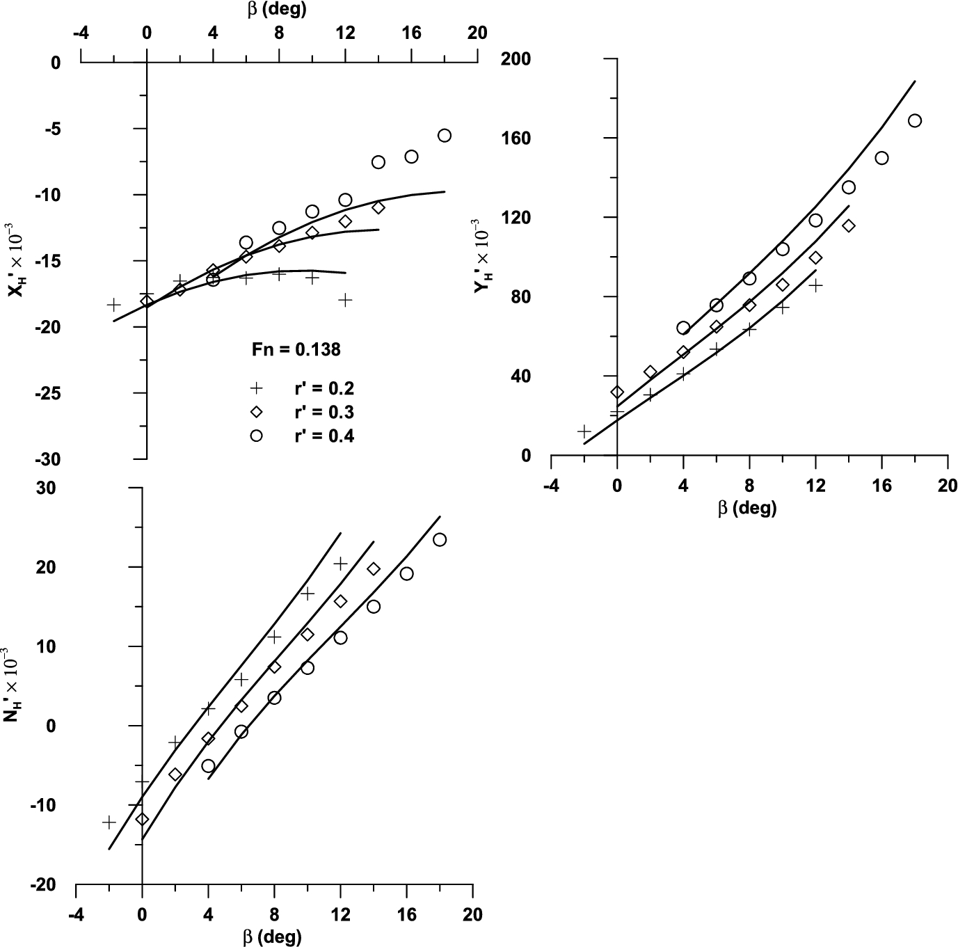
Comparison of model predictions and CMT test data at , BEC [35]. The mathematical model is developed using CMT experimental data corresponding to .
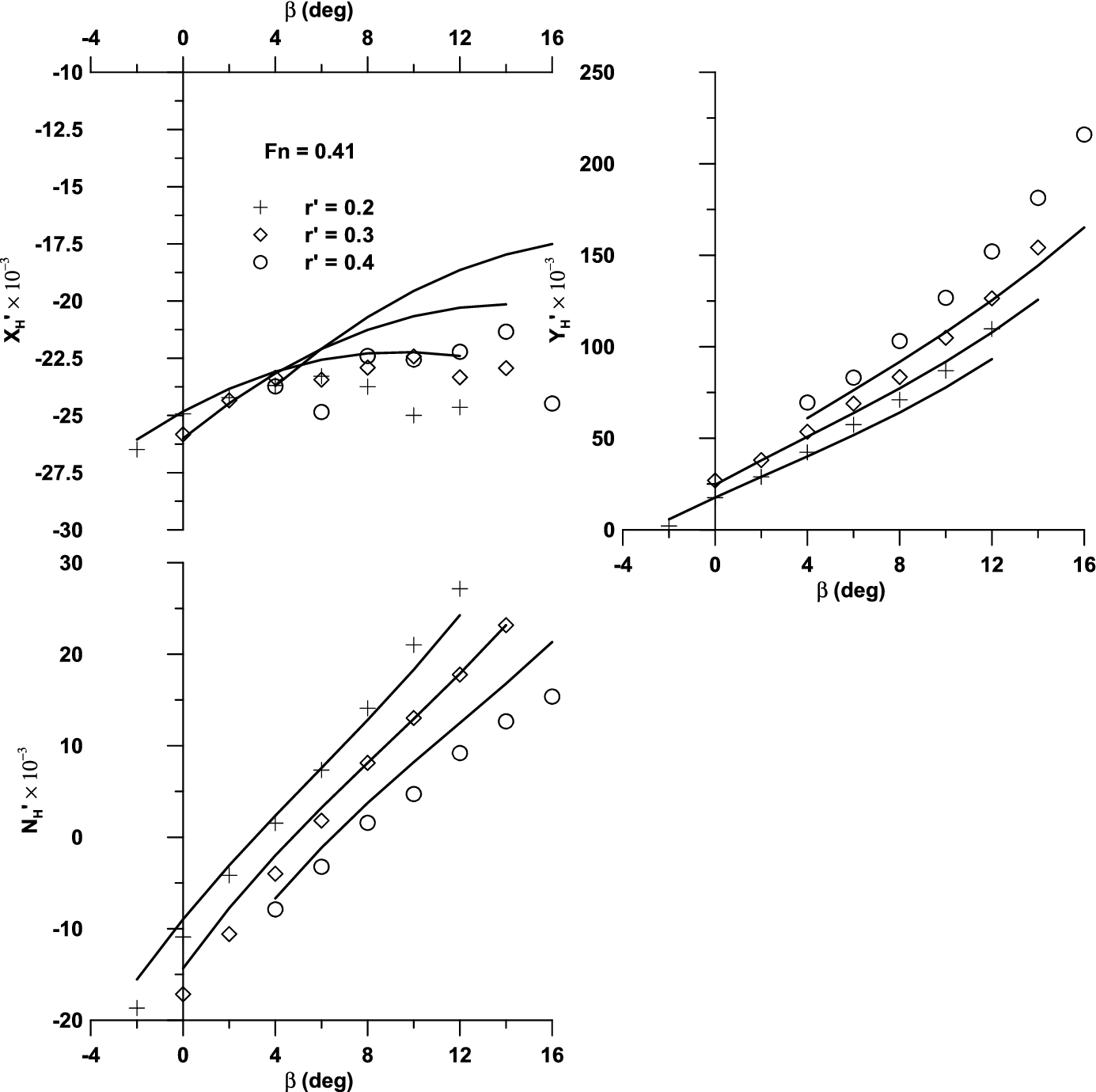
Comparison of model predictions and CMT test data at , BEC [35].
Comparison of model predictions and CMT test data at , BEC [35]. The mathematical model is developed using CMT experimental data corresponding to .
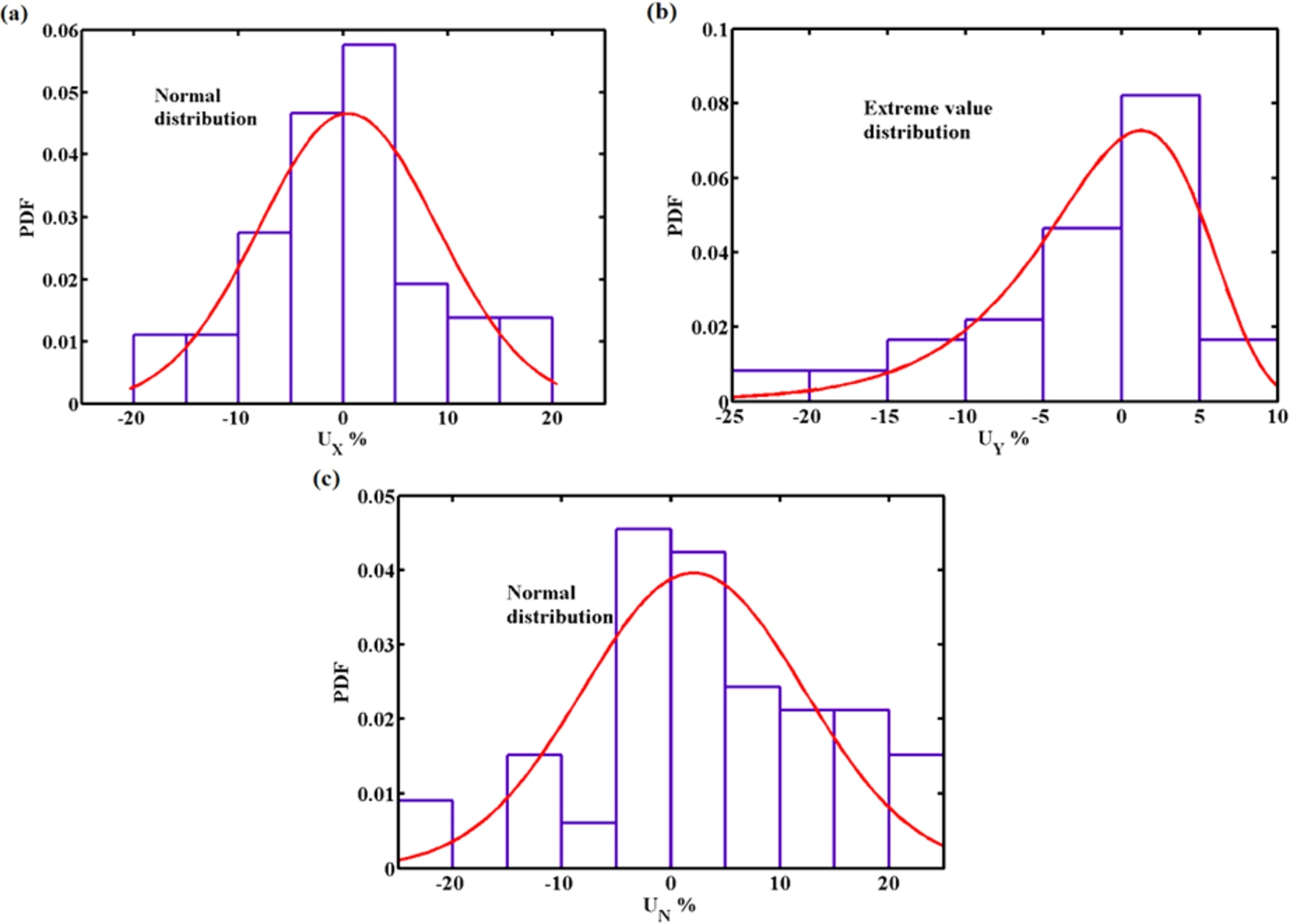
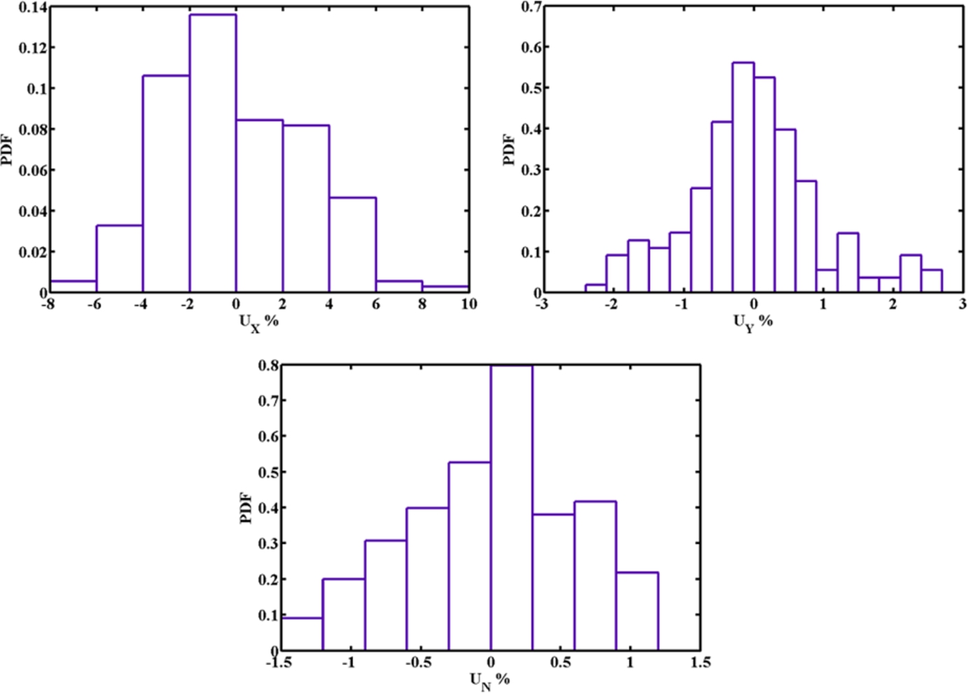
Probability distribution of uncertainty because of speed variation during CMT test. Uncertainty is due to combination of curve fitting uncertainties shown in Figs 2–4. Sample size is 80. Distribution type and parameters: (a) normal, , , (b) extreme value, , and (c) normal, , . (Colors are visible in the online version of the article; http://dx.doi.org/10.3233/ISP-150117.)
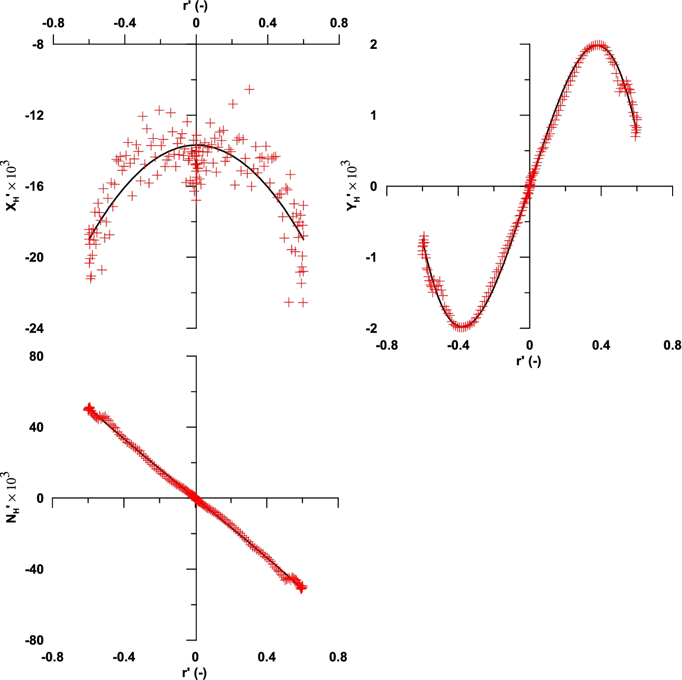
Comparison of mathematical model predictions and pure yaw test data at and [33]. (Colors are visible in the online version of the article; http://dx.doi.org/10.3233/ISP-150117.)
Probability distribution of experimental uncertainty during pure yaw test. Experimental results are shown in Fig. 6. Sample size is 200. (Colors are visible in the online version of the article; http://dx.doi.org/10.3233/ISP-150117.)
Probability distribution of mathematical modeling uncertainty during pure yaw test. Experimental results are shown in Fig. 6. Sample size is 200. (Colors are visible in the online version of the article; http://dx.doi.org/10.3233/ISP-150117.)
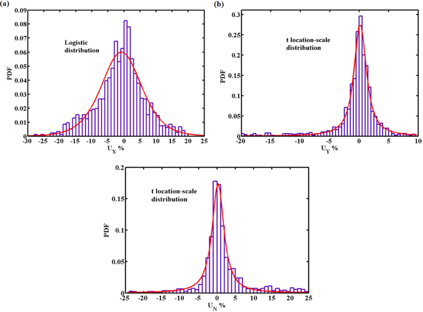
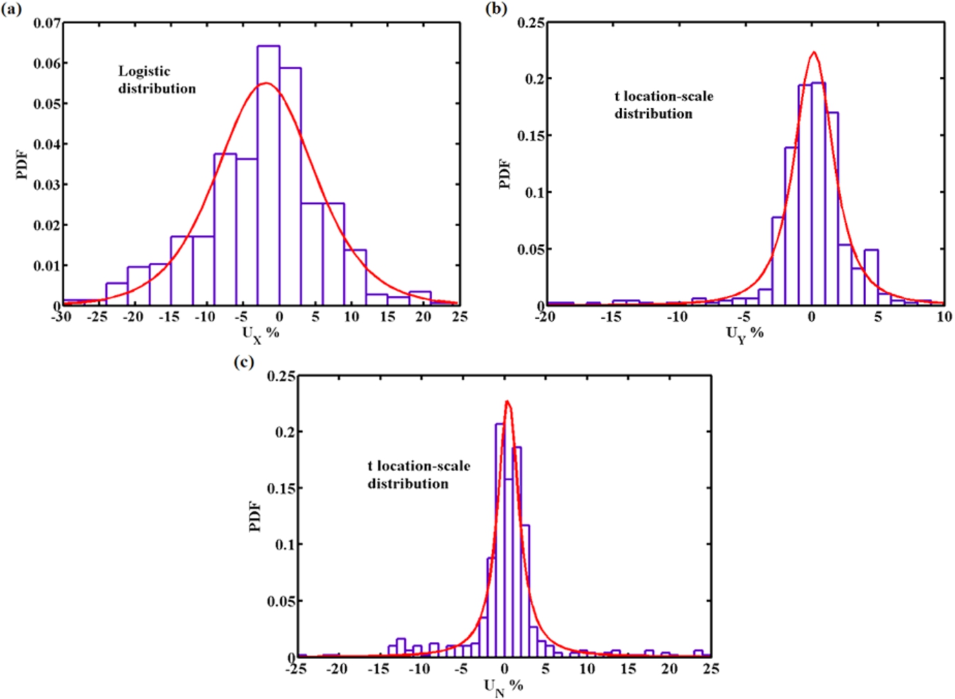
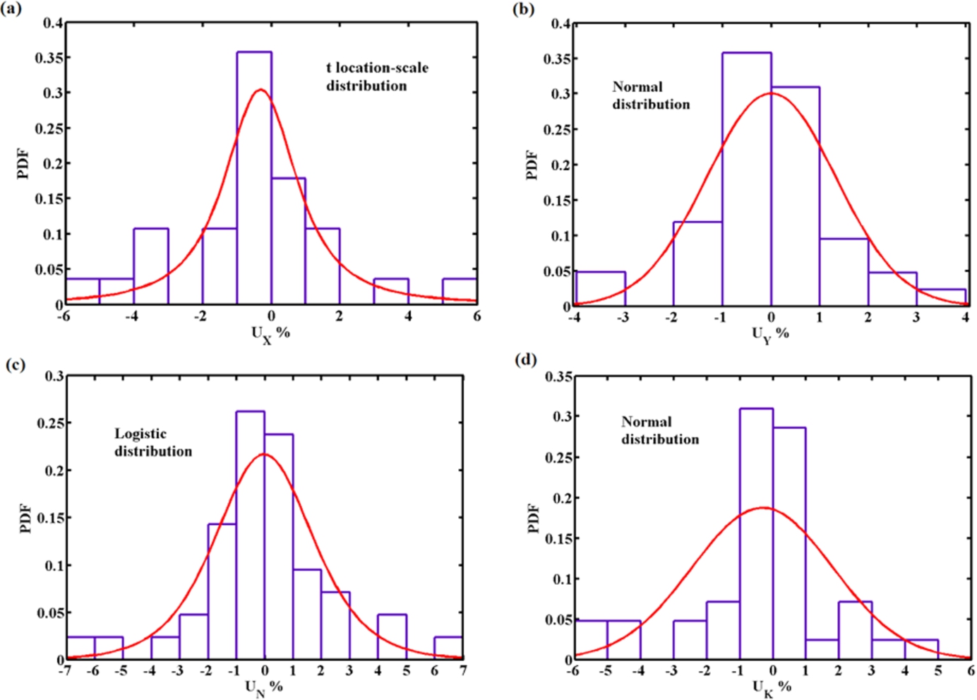
Probability distribution of total uncertainty during pure yaw test. It is the combination of uncertainties shown in Figs 5, 7, and 8. Sample size is 600. Distribution type and parameters: (a) logistic, , , (b) t location-scale, , , and (c) t location-scale, , , . (Colors are visible in the online version of the article; http://dx.doi.org/10.3233/ISP-150117.)
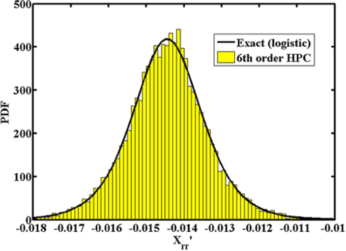
Probability density of . (Colors are visible in the online version of the article; http://dx.doi.org/10.3233/ISP-150117.)
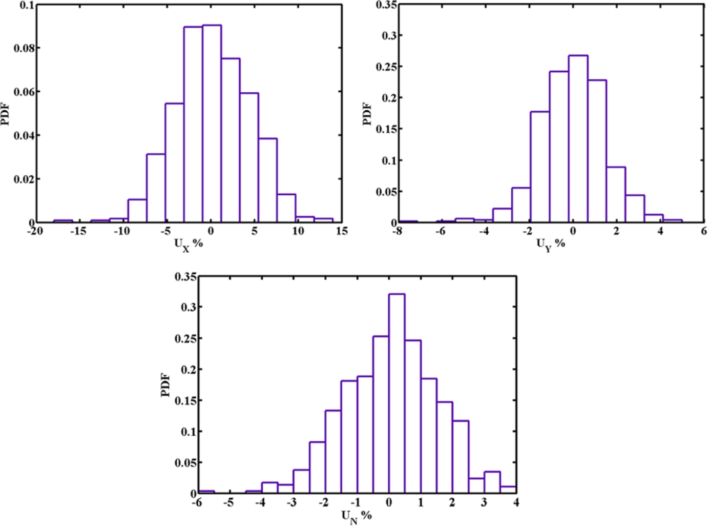
CMT test data at , at are available (80 samples) [35]. Tests are conducted for bare hull in steady-state condition. This data is used to calculate . Data at are fitted with a 3 DoF mathematical model as shown in Fig. 2. The same mathematical model is used for comparing the model predictions over experimental data at as shown in Figs 3 and 4, respectively. The difference between model predictions and experimental values is considered as speed-variation uncertainty. Probability densities of in , and are shown in Fig. 5. The type of probability distribution is assumed to be normal for surge force; extreme value for sway force; and normal for yaw moment.
Comparison of model predictions and static drift test data at and [33]. (Colors are visible in the online version of the article; http://dx.doi.org/10.3233/ISP-150117.)
Probability distribution of experimental uncertainty during static drift test. Experimental results are shown in Fig. 11. Sample size is 200. (Colors are visible in the online version of the article; http://dx.doi.org/10.3233/ISP-150117.)
Probability distribution of mathematical modeling uncertainty during static drift test. Experimental results are shown in Fig. 11. Sample size is 200. (Colors are visible in the online version of the article; http://dx.doi.org/10.3233/ISP-150117.)
Probability distribution of total uncertainty during static drift test. It is the combination of uncertainty shown in Figs 5, 12 and 13. Sample size is 600. Distribution type and parameters: (a) logistic, , , (b) t location-scale, , , and (c) t location-scale, , , . (Colors are visible in the online version of the article; http://dx.doi.org/10.3233/ISP-150117.)
Comparison of mathematical model predictions and drift + yaw test data at , and [33]. Sample size is 100. (Colors are visible in the online version of the article; http://dx.doi.org/10.3233/ISP-150117.)
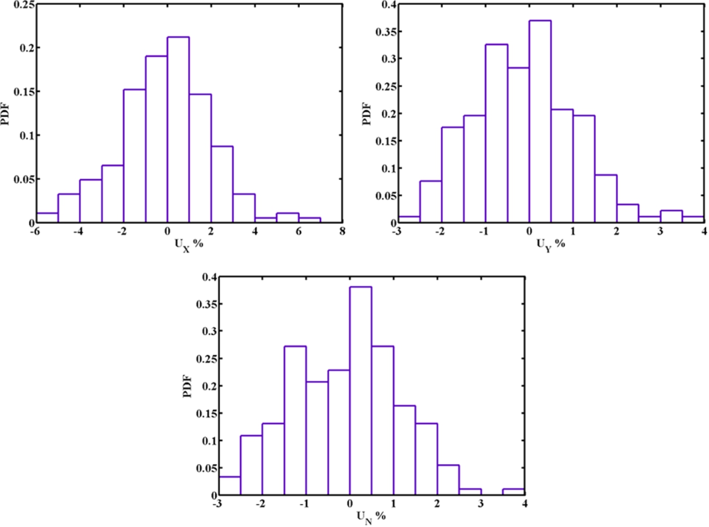
Probability distribution of experimental uncertainty during drift + yaw test. Experimental results are shown in Fig. 15. Sample size is 100. (Colors are visible in the online version of the article; http://dx.doi.org/10.3233/ISP-150117.)
Probability distribution of mathematical modeling uncertainty during drift + yaw test. Experimental results are shown in Fig. 15. Sample size is 100. (Colors are visible in the online version of the article; http://dx.doi.org/10.3233/ISP-150117.)
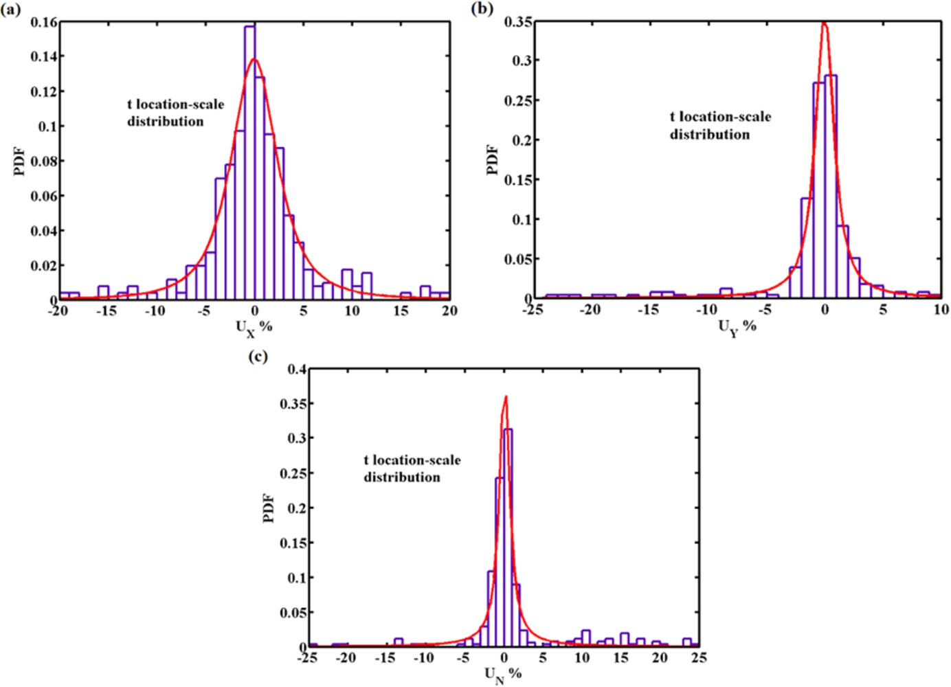
Probability distribution of total uncertainty during drift + yaw test. It is the combination of uncertainties shown in Figs 5, 16 and 17. Sample size is 300. Distribution type and parameters: (a) t location-scale, , , , (b) t location-scale, , , and (c) t location-scale, , , . (Colors are visible in the online version of the article; http://dx.doi.org/10.3233/ISP-150117.)
Comparison of model predictions and drift + heel test data at , , and and 0.329 [28]. Sample size is 27. (Colors are visible in the online version of the article; http://dx.doi.org/10.3233/ISP-150117.)
Probability distribution of experimental uncertainty during drift + heel test. Experimental results are shown in Fig. 19. Sample size is 56. (Colors are visible in the online version of the article; http://dx.doi.org/10.3233/ISP-150117.)
Probability distribution of mathematical modeling uncertainty during drift + heel test. Experimental results are shown in Fig. 19. Sample size is 27. (Colors are visible in the online version of the article; http://dx.doi.org/10.3233/ISP-150117.)
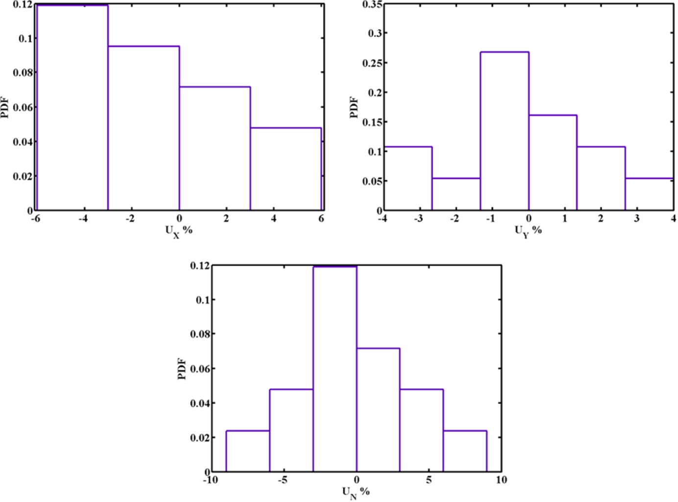
Probability distribution of total uncertainty during drift + heel test. It is the combination of uncertainties shown in Figs 20 and 21. Sample size is 81. Distribution type and parameters: (a) t location-scale, , , , (b) normal, , , (c) logistic, , and (d) normal, , . (Colors are visible in the online version of the article; http://dx.doi.org/10.3233/ISP-150117.)
Comparison of model predictions and yaw + heel test data at (at ) and 0.9 (at ), [28]. (Colors are visible in the online version of the article; http://dx.doi.org/10.3233/ISP-150117.)
Probability distribution of experimental uncertainty during yaw + heel test. Experimental results are shown in Fig. 23. Sample size is 30. (Colors are visible in the online version of the article; http://dx.doi.org/10.3233/ISP-150117.)
Probability distribution of mathematical modeling uncertainty during yaw + heel test. Experimental results are shown in Fig. 23. Sample size is 15. (Colors are visible in the online version of the article; http://dx.doi.org/10.3233/ISP-150117.)
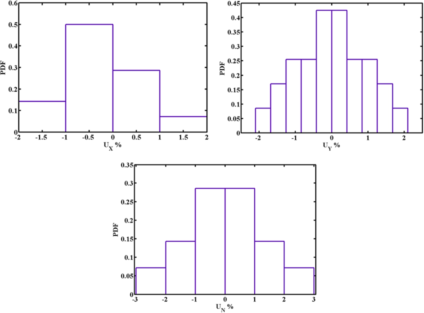
Probability distribution of total uncertainty during yaw + heel test. It is the combination of uncertainties shown in Figs 24 and 25. Sample size is 45. Distribution type and parameters: (a) t location-scale, , , , (b) t location-scale, , , and (c) normal, , . (Colors are visible in the online version of the article; http://dx.doi.org/10.3233/ISP-150117.)
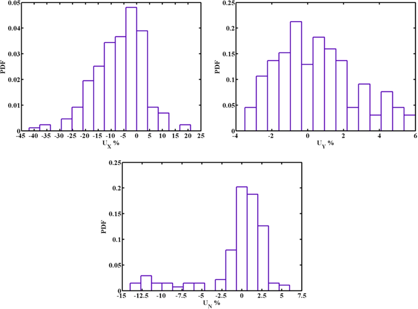
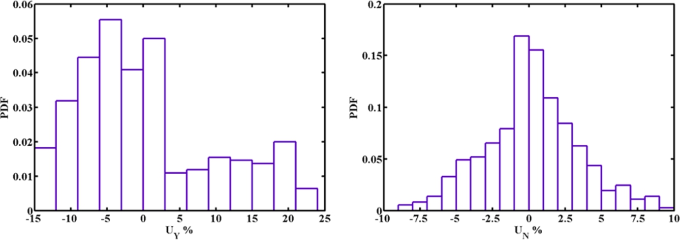
Pure yaw test data are available for (200 samples) [33]. , , , and are calculated by the least square fit of , and with the mathematical model. Comparison between model predictions and the pure yaw test data is shown in Fig. 6. The variation of data is symmetry for positive and negative for surge and sway forces and yaw moment. The scatter among the data is higher for the surge force. Sudden drop in after is observed similar to the stall phenomenon for aerofoil. is calculated for surge and sway force and yaw moment and the probability distribution is shown in Fig. 7. is calculated for surge and sway force and yaw moment and the probability distribution is shown in Fig. 8. for pure yaw test is considered as similar to the values shown in Fig. 5. The distribution of the total uncertainties for the three parameters, i.e. in , and is shown in Fig. 9. The type of probability distribution is assumed to be logistic for surge force; t location-scale for sway force and yaw moment. Uncertainty is more in then and . It is assumed that the distribution of uncertainty in is same as that of ; and is same as that of ; and is same as that of in Fig. 9. HPC expansion for is given in Eq. (24). HPC expansion of is sampled 105 times by MCS method. Comparison of probability distribution of HPC sampling data and exact distribution of is shown in Fig. 10. The probability density of HPC sampling data matches well with exact distribution,
Static drift test data are available for (200 samples) [33]. , , , and are calculated by least square fit of , and with the mathematical model. Comparison between model predictions and the static drift test data is shown in Fig. 11. The experiment data is symmetric for positive and negative β. Significant noise is observed in . Non-linearity in and is observed after . is calculated for each data point and its probability distribution is shown in Fig. 12. is calculated for surge force, sway force and yaw moment and its probability distribution is shown in Fig. 13. Distribution of for static drift test is considered similar to that shown in Fig. 5. Distribution of the three types of uncertainties together, i.e. for , and is shown in Fig. 14. The type of probability distribution is assumed to be normal for surge force; extreme value for sway force; and normal for yaw moment. Uncertainty is higher for as compared to and . For analysis, we assume that the distribution of uncertainty in is same as that of ; and is same as that of ; and is same as that of in Fig. 14.
Drift + yaw test data are available for , (100 samples) [33]. Linear and non-linear model coefficients related to drift and yaw are extracted from static drift and pure yaw tests, respectively. By keeping these coefficients’ value same, the coupling coefficients are calculated from drift + yaw tests. This procedure works better to get accurate values for most of the coefficients. , , , and are calculated by least square fit of , and with the mathematical model. Comparison between model predictions and the drift + yaw test data is shown in Fig. 15. The scatter in the value of is observed to be higher as compared to other data. is calculated for each measured parameter and their probability distribution is shown in Fig. 16. is calculated for each of the measured parameter and their probability distribution is shown in Fig. 17. for drift + yaw test data is considered same as shown in Fig. 5. The probability distribution of the total uncertainty for the three parameters i.e. , for , and is shown in Fig. 18. The type of probability distribution is assumed to be t location-scale distribution for surge force, sway force and yaw moment. It is observed that uncertainty is more in as compared to and . It is assumed that the distribution of uncertainty in is same as that of ; and is same as that of ; and is same as that of in Fig. 18.
Uncertainties in roll-related coefficients are studied. The bias limit for roll moment transducer is not known. Therefore, for could not be calculated in roll-related tests. for is same as . Drift + heel test data are available for , at (27 samples) [28]. , , , , , , , , , , , , are calculated by least square fit of , , and with the mathematical model. Comparison between model prediction and the drift + heel test data is shown in Fig. 19. It is observed that the model well predicts the variation observed in experiment. It may be noted that the static heel experiments are carried out by Force in appended hull condition. In appended hull condition, the propeller and rudder are working. Therefore, to get the bare hull coefficients, the rudder and propeller forces and moment must be deducted from the measured hull forces. This increases the error in estimation of these coefficients. is calculated for each measured parameter and their probability distribution is shown in Fig. 20. is calculated for each measured parameter and their probability distribution is shown in Fig. 21. Both are combined statistically to get in , , and (see Fig. 22). The type of probability distribution is assumed to be t location-scale distribution for surge force; normal for sway force; logistic for yaw moment; and normal for roll moment. It is assumed that the distribution of uncertainty in is same as that of ; , , and is same as that of ; , , and is same as that of ; , , and is same as that of in Fig. 22. Yaw + heel test data are available for , and (15 samples) [28]. , , , , and are calculated by least square fit of , and with the mathematical model. Comparison between model predictions and the yaw + heel test data is shown in Fig. 23. is calculated for each measured parameter and their probability distribution is shown in Fig. 24. is calculated for each measured parameter and their probability distribution is shown in Fig. 25. Both are combined statistically to get in , and (see Fig. 26). Uncertainty is more in as compared to and . It is assumed that the distribution of uncertainty in and is same as that of ; and is same as that of ; and is same as that of in Fig. 26. The ship maneuvering coefficients for DTMB 5415 are given in Table 6.
Twin-rudder and twin-propeller model and uncertainty
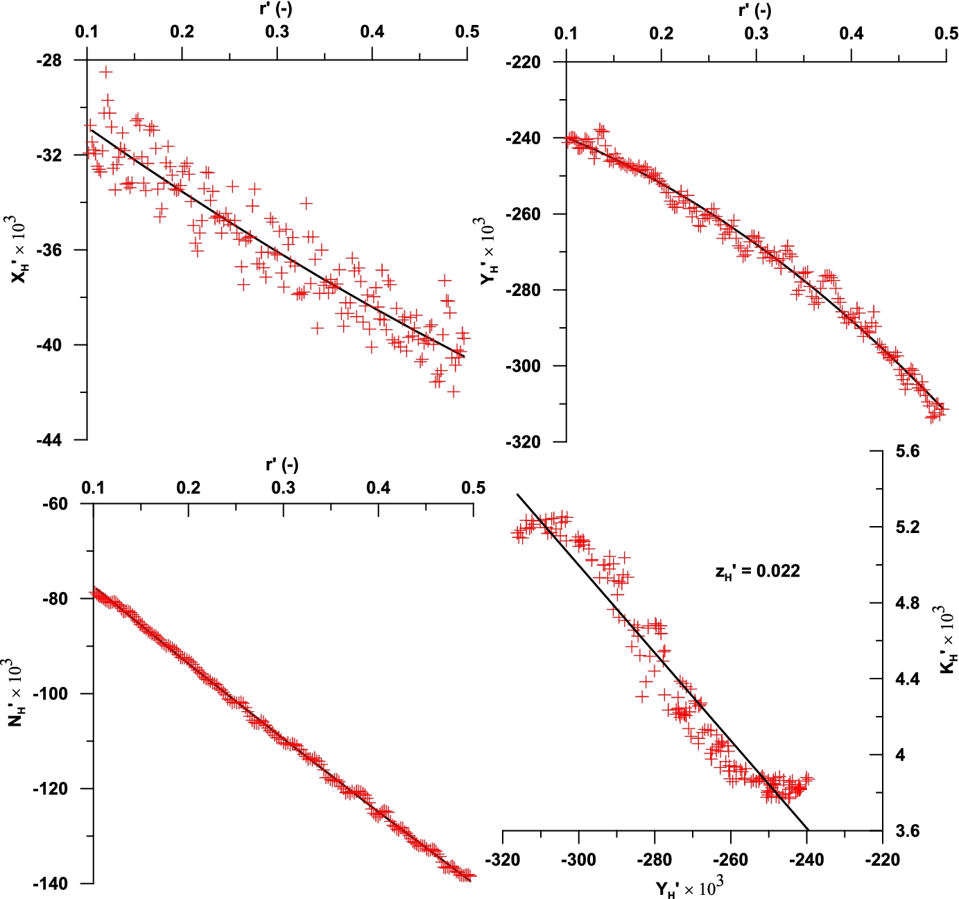
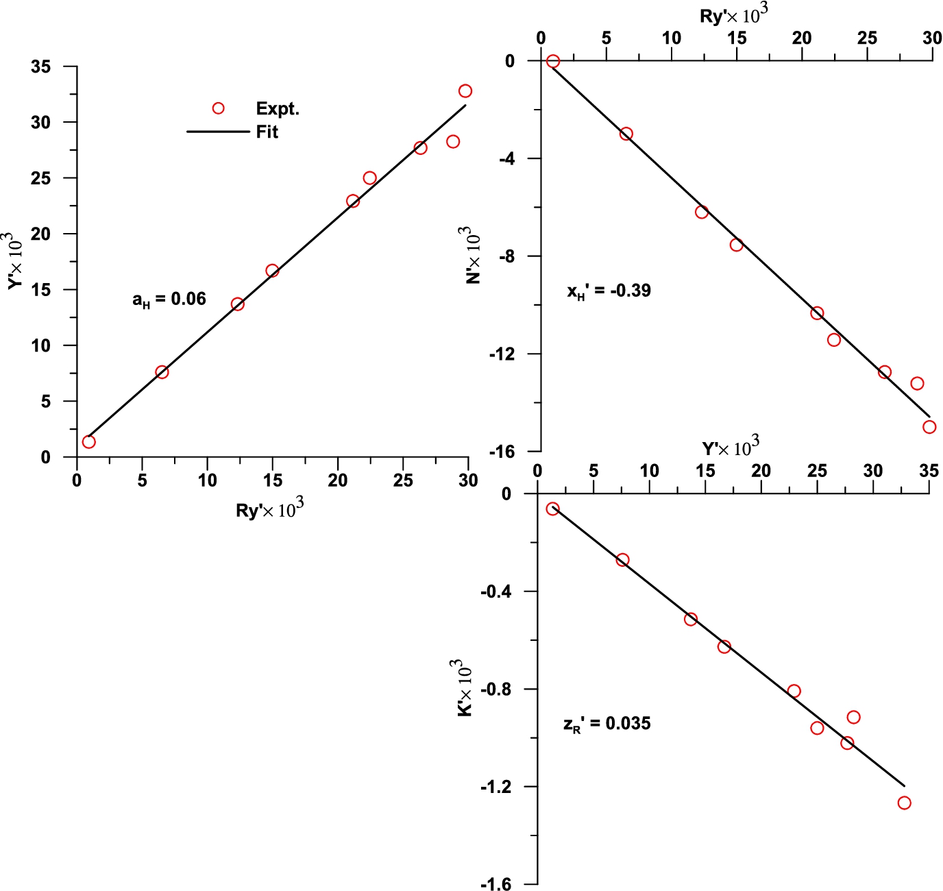
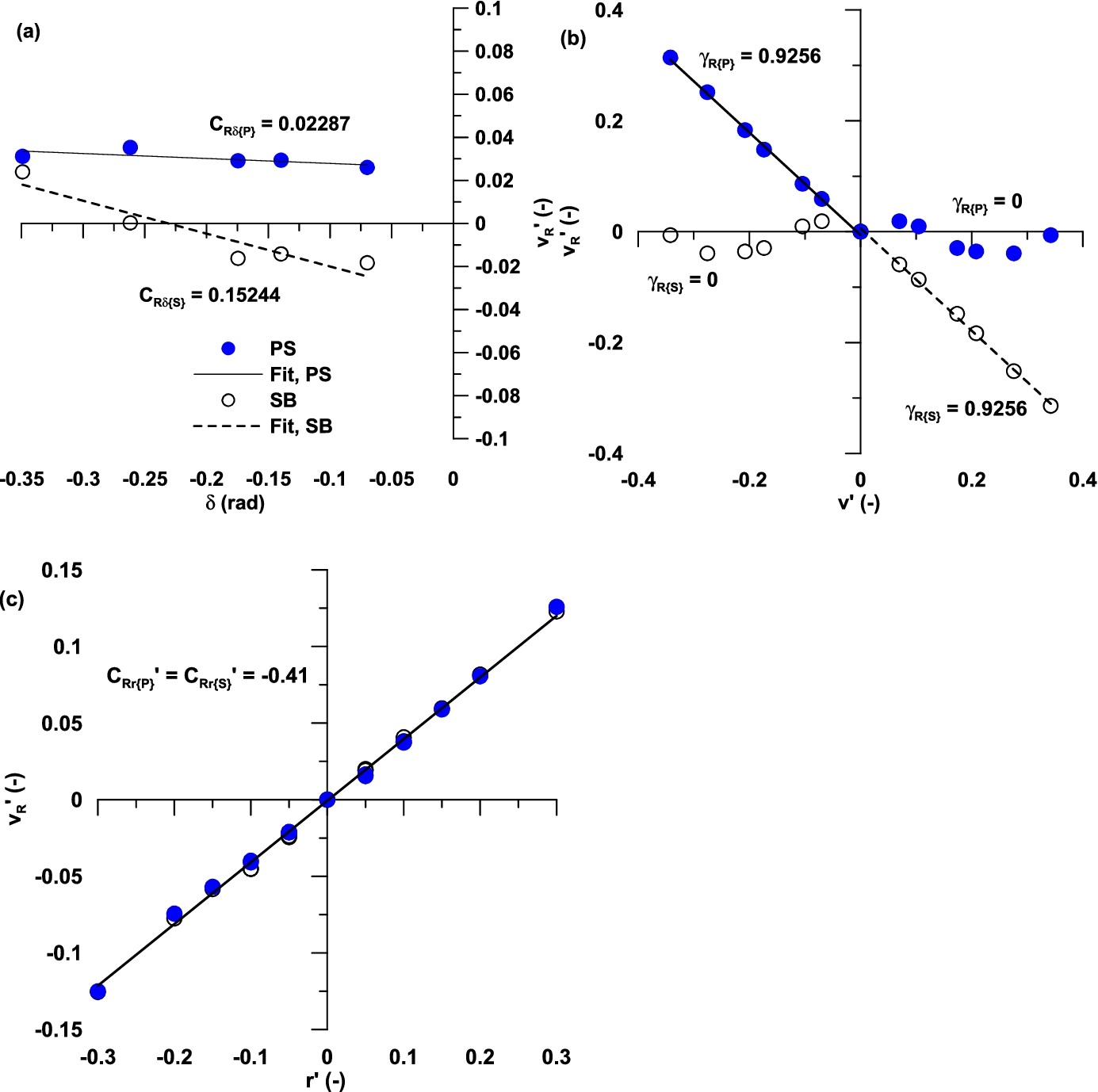
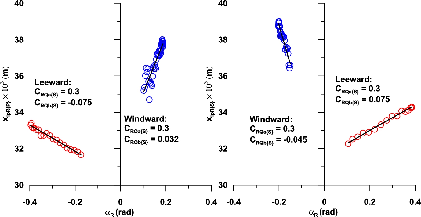
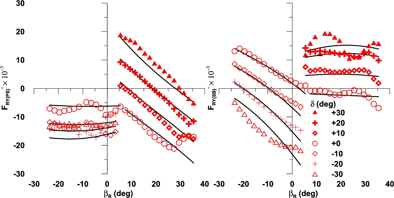
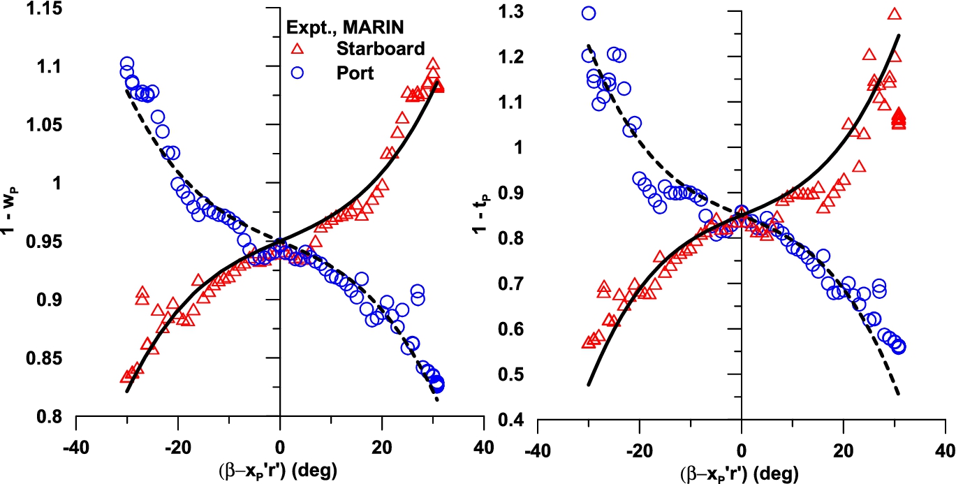
The interaction coefficients related to twin-propeller and twin-rudder models are calculated using MARIN’s [33] appended hull test data. When the ship turns to port side, the port rudder/propeller is the leeward side and starboard rudder/propeller is the windward side. For turns to starboard side, the opposite is true. For maneuvering of ships with twin-propeller and twin-rudder, the two rudders or propellers do not get same flow field. Because of this reason, both twin-rudder and twin-propeller may exhibit asymmetric characteristics during port or starboard maneuvering. This aspect is investigated using the available experimental data. Static rudder test data at are used for calculating the coefficients , ε, κ, , and . Hill climbing technique [24] is used to calculate , ε and κ from rudder normal force data at . The estimated value of , and is shown in Fig. 27. Rudder inflow straightening coefficients , and corresponding to the rudder, sway and yaw motions respectively are shown in Fig. 28. Static rudder test data is analyzed. It is seen that the leeward rudder gets maximum inflow and hence generates larger forces (in magnitude) as compared to windward rudder. It can be said that the straightening of inflow to leeward side is more [32]. Therefore, the effective angle of attack is more for leeward side rudder. is calculated from static rudder test data for windward and leeward side rudder. Static drift test data is analyzed. The rudder angle is kept zero. It is seen that leeward rudder gets minimum inflow and hence generates smaller forces (in magnitude) as compared to the windward rudder. It can be said that the straightening of inflow to leeward side is less. Therefore, the effective angle of attack reduces for leeward rudder. is calculated from static drift test data for windward and leeward side rudder. Pure yaw test data are analyzed. It is seen that both rudders get similar flow field, i.e. flow asymmetry between lee and windward rudders vanishes. Therefore, both rudders generate similar forces (in magnitude). is calculated from pure yaw test data. The value of is same for windward and leeward rudders. Determination of coefficients present in the mathematical model of center of pressure on the rudder is shown in Fig. 29. When the effective angle of attack to rudder is +ve (towards the starboard side), the center of pressure on rudder shifts towards the trailing edge. Similarly, when the effective angle of attack to rudder is −ve (towards the port side), center of pressure shifts towards the leading edge. The hull, rudder and propeller interaction coefficients are given in Table 7. It is seen that both the numeral value and direction of torque are usually different. It is possible to have separate or a single steering gear unit for port and starboard rudders [10] based on cost, space, weight considerations. In case a single steering gear unit is opted for, the rudders can only be operated in a synchronized manner. In such cases, the variation in torque load may be high. In addition, the total load may not be twice of the individual torque load. If, they are in the same direction, torque load will be the maximum of the two. If it is in the opposite direction, then the torque load will be the addition of the absolute values. Therefore, the load estimation needs to be carried out carefully. Advantages of separate steering gear in asymmetric operation will be described later. Comparison between model predictions and experimental values of twin-rudder normal force is shown in Fig. 30. The rudder forces are asymmetric for port and starboard maneuvers. It is observed that the rudder model closely approximates the experimental values for windward rudders. For the leeward rudder at an angle more than 20°, the rudder normal force is not steady, so the modeling is not proper. At the rudder angle greater than 10°, the sway inflow velocity to rudder is influenced by the opposite rudder angle. The experiment results show that torque is not uniform for port and starboard rudders even though both the rudders are operated in a synchronized manner. In the model experiment, it is ensured that the rudder stock directly connects to the load cell without touching any other structure. This ensures that all the hydrodynamic force and torque are measured. In the ship, there is an additional torque load on the steering gear machinery due to friction in support bearings. For single-rudder system, displacing and restoring torques are different due to the location of the rudder stock along the chord [14]. In case of twin-rudder system, there is additional discontinuity in the torque for port and starboard turn. This aspect needs to be considered in design of steering gear. If it is intended to fit a single steering gear unit for minimizing cost and weight, then it must be considered that the maximum torque load on the steering gear will be lower than two times of the maximum individual rudder torque (hydrodynamic + frictional). The displacing and restoring torque pattern will be asymmetric and discontinuous. Distributions of in windward and leeward side rudder normal forces are given in Fig. 31. is more in leeward side rudder normal force model. The type of probability distribution is assumed generalized extreme value distribution for windward and normal for leeward rudder normal.
The open water characteristics of FORCE propeller number 6515 are given in Table 8. Comparison between model predictions of the propeller effective wake and thrust deduction fraction and the experimental data are shown in Fig. 32. is calculated for each measured parameter and their probability distribution is shown in Fig. 33. is higher for thrust deduction fraction as compared to effective propeller wake. The type of probability distribution is assumed to be normal for and t location-scale distribution for . Comparison between the propeller thrust and torque model prediction and the experimental data during maneuvering condition is shown in Fig. 34. It is observed that the propeller thrust and torque are asymmetric for port and starboard maneuvers. For single-propeller ship, the variation of thrust and torque during maneuvering motions is well known [15]. For twin-propeller ship besides, the variation of thrust and torque during maneuvering motion, there is an additional asymmetry depending on the ship’s port or starboard turn. The differential propeller thrust may cause an extra turning moment on the hull. The difference in the port and starboard torque will cause different loading on the prime mover. Therefore, the port and starboard prime mover needs to be controlled independently. In case a single prime mover is intended for minimizing weight and cost, there will be no difference in port and starboard propeller revolution. The total torque load needs to be separately estimated for this configuration.
Validation and predictions
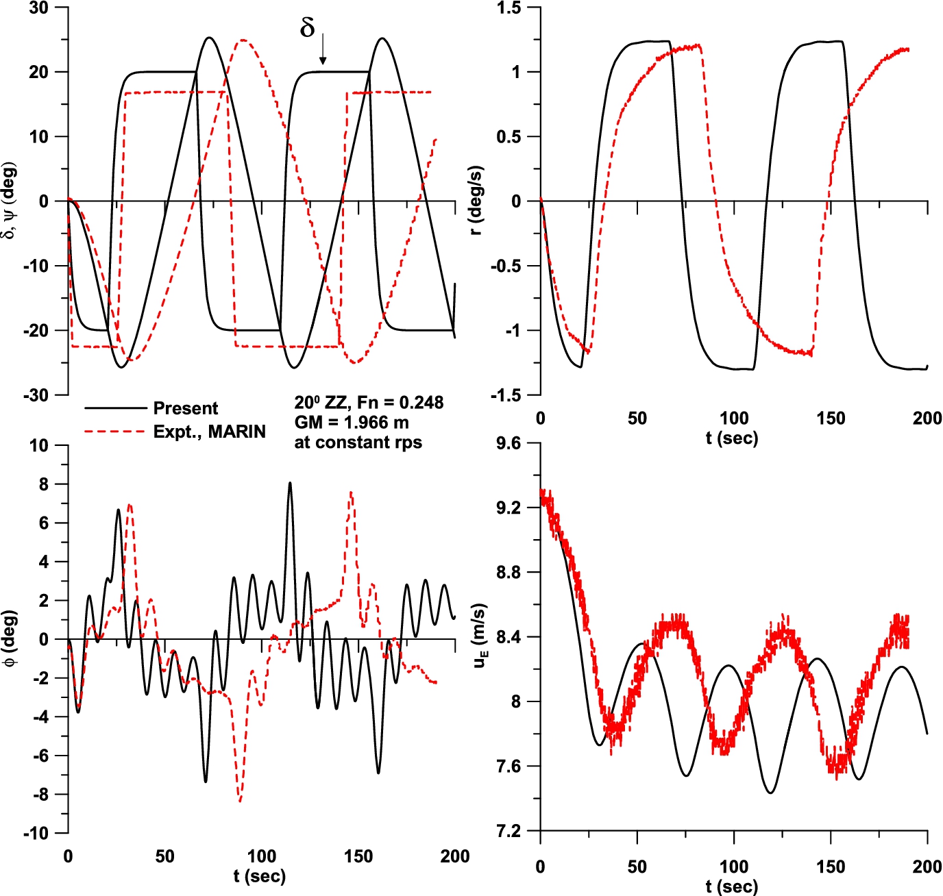
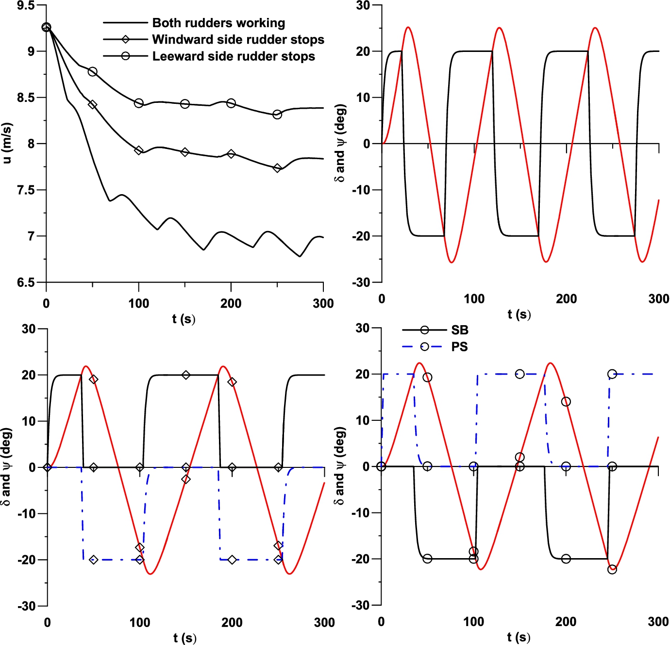
Full-scale simulations of 20° zigzag maneuvers at using constant propeller revolution are validated against the free running experimental data [33]. The model experimental data has been extrapolated and presented as full-scale data. The comparison of heading angle, yaw rate and roll angle is shown in Fig. 35. We can see a good agreement of predicted values with model free run test data. The full-scale zigzag maneuvers at constant propeller torque will be studied. As the flow becomes asymmetric over the propeller and rudder during maneuvering, we devise some new operating procedures for the rudder to better utilize their output. Three cases of twin-rudder behaviors are considered during maneuvers; those are: (1) both rudders are working, (2) the leeward side rudder working and windward side rudder angle is zero; and (3) the windward side rudder is working and leeward side rudder angle is zero. The time series of longitudinal speed drop, heading, rudder and roll angle are shown in Fig. 36. In the cases 2 and 3 speed drop, overshoot angle and maximum roll angle are less as compared to the case 1. The time required to get the desired heading is more. The difference will increase if the gas-turbine propulsion is applied. The time series of propeller revolution and main engine power are shown in Fig. 37. Drop in the propeller revolution and main engine power is less in case 3. For naval ships, reduction of speed drop in higher ship motions may be more critical in certain circumstances. For optimal maneuvering the possibility of asymmetric operation of the twin-rudder twin-propeller system may be considered.
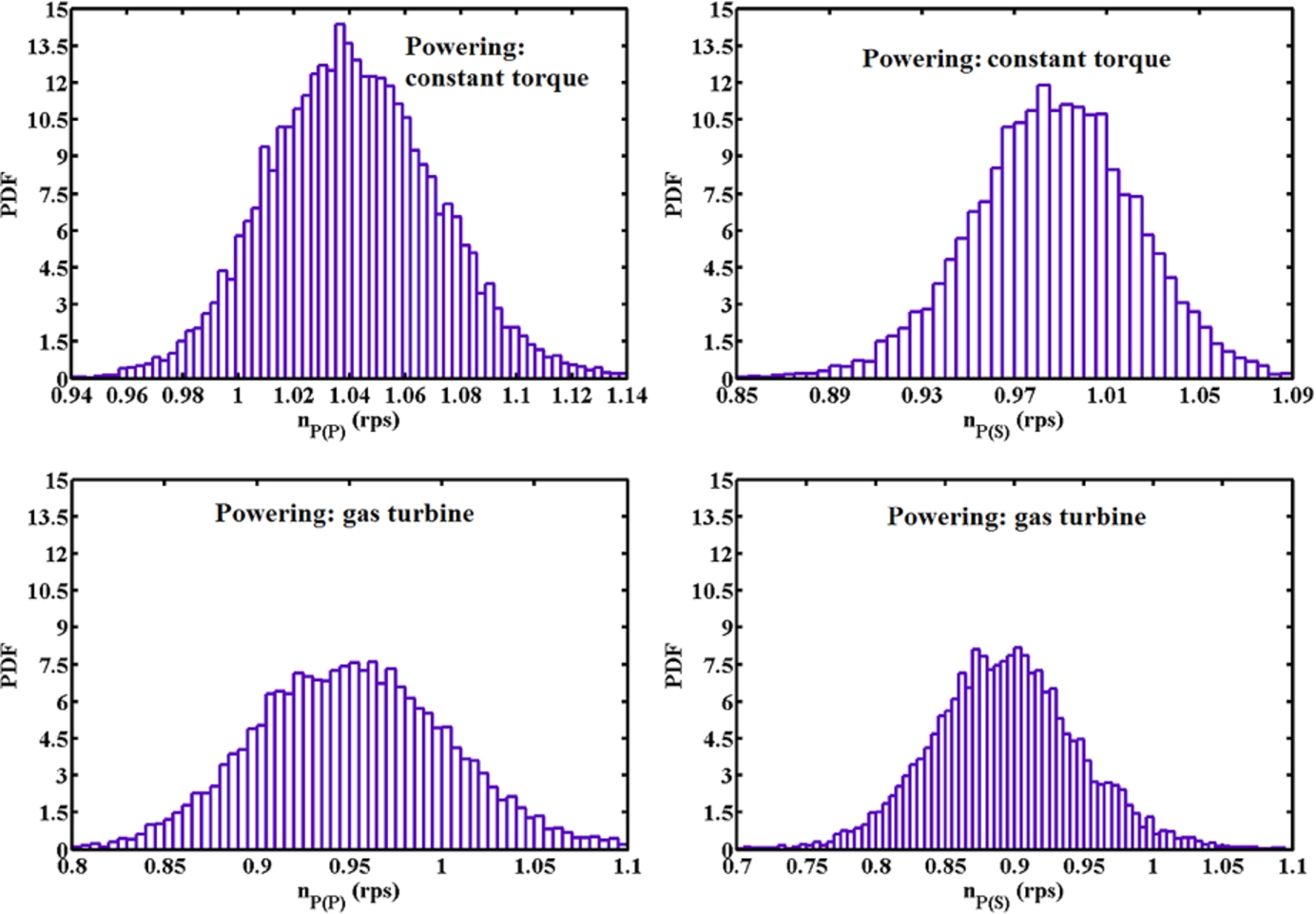
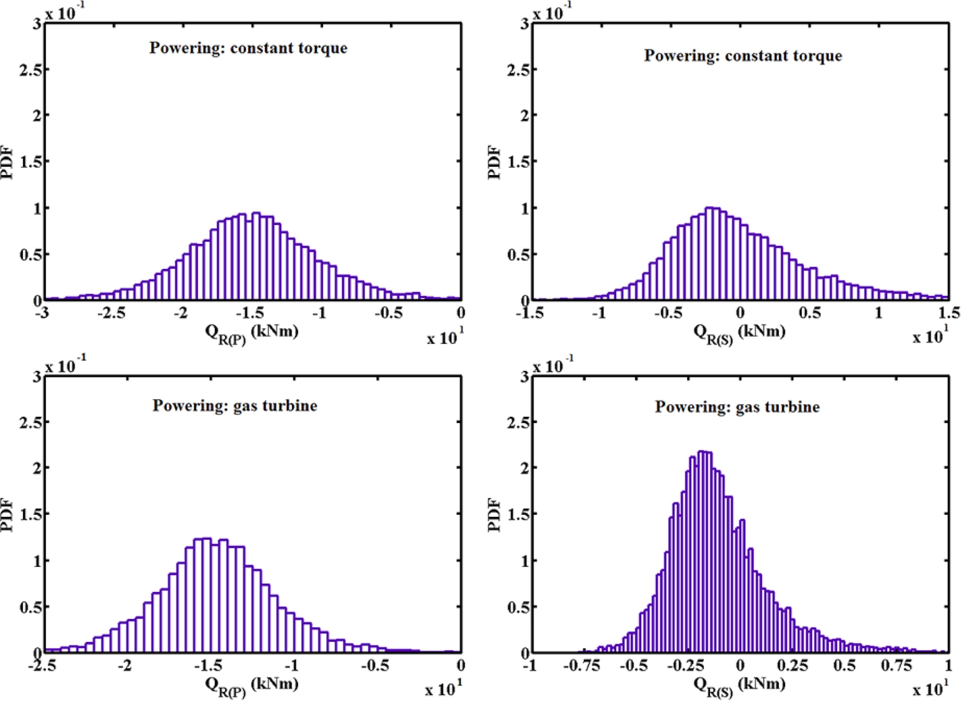
Uncertainty in model coefficients is propagated to full-scale simulations of 20° zigzag maneuver at using standard Monte Carlo simulation method. Simulation is repeated to collect 105 samples. Uncertainty in propeller revolution, main engine power and rudder torque will be studied. We considered both the diesel engine and gas-turbine prime mover configuration. The probability distribution of propeller revolution is shown in Fig. 38. The distribution is shown to correspond to the time instant . In both cases, the uncertainty for the port and starboard shaft revolution is different. The distribution has slightly changed depending on the type of the prime mover. The controller used for the prime mover must be suitable to handle such fluctuations in the output. Uncertainty in starboard propeller revolution is 7.36%–6.93% (at constant torque strategy) and 11.25%–12% (at gas-turbine strategy) of the deterministic value at 95% confidence interval. Uncertainty in port propeller revolution is 5.72%–6.06% (at constant torque strategy) and 10.39%–11.29% (at gas-turbine strategy) of the deterministic value at 95% confidence interval. The probability distribution of power of the prime mover is shown in Fig. 39. The distribution is shown corresponding to the time instant . In both cases, the uncertainty for the port and starboard power is different. The distribution has slightly changed depending on the type of the prime mover. The controller used for the prime mover must be suitable to handle such fluctuations in the output. Uncertainty in starboard engine power is 10.61%–12.63% (at constant torque strategy) and 21.10%–26% (at gas-turbine strategy) of the deterministic value at 95% confidence interval. Uncertainty in port engine power is 14.6%–14.2% (at constant torque strategy) and 19.7%–23.65% (at gas-turbine strategy) of the deterministic value at 95% confidence interval. The probability distribution of rudder torque is shown in Fig. 40. The distribution is shown corresponding to the time instant . In both cases, the uncertainty for the port and starboard torques are different. Uncertainty in gas-turbine control strategy is higher than constant torque control strategy. In both cases, the probability distribution shows that port rudder torque will be negative. In case of starboard torque, for both the cases, the probability distribution shows that starboard rudder torque may be either positive or negative. Therefore, the load on port and starboard steering gear will be different.
Conclusions
Uncertainty assessment of maneuvering model of twin-propeller twin-rudder surface combatant DTMB 5415 is investigated in this paper. The following are the main conclusions of this paper:
Uncertainty due to speed variation is higher as compared to mathematical modeling uncertainty and experimental uncertainty. Non-dimensional hydrodynamic forces and moment vary with speed, type of model and the experiment set up. Uncertainties are higher at lower speed.
Distribution of uncertainty in hydrodynamic forces and moment is different for different captive model tests in bare hull condition.
Propeller interaction coefficients are determined from different appended hull captive model tests. Asymmetry in twin-propeller thrust and torque are observed during captive maneuvering model tests. The asymmetry is modeled. Uncertainties in the interaction coefficients ( and ) are considered and their distributions determined.
Rudder and hull + propeller interaction coefficients are determined from different appended hull captive model tests. Asymmetry in twin-rudder normal force is observed during captive maneuvering model tests. The asymmetry is modeled. Uncertainties in the mathematical model of rudder normal force are computed and their distribution determined. Uncertainty is higher in leeward rudder normal force. Asymmetry is also observed in the location of center of pressure of rudder normal force during captive maneuvering model tests. The asymmetry is modeled.
The asymmetry in rudder model can be utilized for optimal maneuvering. If leeward side rudder is not used, then the speed drop during zigzag maneuver is reduced. The drop in propeller revolution and prime mover power is less in this operating condition.
Uncertainties in maneuvering coefficients are propagated to full-scale zigzag maneuver simulations. Both diesel engine (constant torque) and gas-turbine prime mover configuration are investigated. Uncertainty in propeller revolution, power of prime mover and rudder torque is computed. Uncertainty is higher with gas turbine as the prime mover. At any time, the uncertainty for port propeller thrust and torque is different from starboard propeller thrust and torque. Similarly, at any time, the uncertainty for port rudder normal force and torque is different from starboard rudder normal force and torque.
Ship maneuvering coefficients
Items
Value
Items
Value
Items
Value
−1.6550E−02
−2.4552E+00
3.8422E−01
−5.8910E−02
6.4651E−02
−5.8993E−04
−1.4561E−02
−1.7005E+00
2.3286E−02
−2.2055E−02
−1.1671E−01
−1.7666E−02
6.5426E−03
−5.1760E−01
3.6785E−01
−3.6663E−01
−8.2431E−02
6.8270E−02
−2.0415E+00
−8.3312E−03
2.6323E−01
3.7452E−02
−1.0234E−04
−1.1576E−01
−1.0412E−02
−4.2441E−02
−1.5494E−02
−2.0169E−02
−1.5637E+00
−9.8130E−03
−1.2014E−01
−5.3745E−01
−1.0008E−02
−8.2264E−01
−5.8824E−01
−2.6600E−04
−3.6761E−01
2.1091E+00
2.2100E−02
1.3927E+00
7.6866E−03
Interaction coefficients of TPTR model
0.150
For
1.00
0.050
0.100
0.108
−0.410
0.500
−0.410
0.267
0.153
1.625
0.023
0.063
For
−0.700
−0.391
For
−0.700
0.035
For
−0.075
ε
0.925
For
0.032
K
0.650
For
−0.045
0.3
For
0.075
0.3
Propeller open water data of FORCE propeller number 6515
Items
Model-scale
Full-scale
Items
Model-scale
Full-scale
0.6744
0.6757
0.1356
0.1349
−0.3440
−0.3440
−0.0683
−0.0683
−0.0934
−0.0934
−0.0143
−0.0143
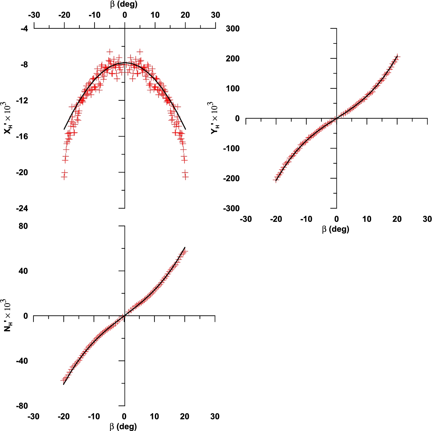
Determination of hull–rudder interaction coefficients , and from static rudder test data [33]. (Colors are visible in the online version of the article; http://dx.doi.org/10.3233/ISP-150117.)
Determination of rudder flow straightening coefficients from appended hull test data [33]. (a) from static rudder test, (b) from drift test and (c) from pure yaw test data. (Colors are visible in the online version of the article; http://dx.doi.org/10.3233/ISP-150117.)
Determination of coefficients present in mathematical model of centre of pressure on rudder. (Colors are visible in the online version of the article; http://dx.doi.org/10.3233/ISP-150117.)
Comparison of model predictions and experimental rudder normal forces at and at [33]. (Colors are visible in the online version of the article; http://dx.doi.org/10.3233/ISP-150117.)
Probability distribution of mathematical modeling uncertainty in rudder normal force: (a) for windward rudder and (b) for leeward rudder. Sample size is 120. Distribution type and parameters: (a) generalized extreme value, , , and (b) normal, , . (Colors are visible in the online version of the article; http://dx.doi.org/10.3233/ISP-150117.)
Determination of propeller effective wake and thrust deduction fraction mathematical model. (Colors are visible in the online version of the article; http://dx.doi.org/10.3233/ISP-150117.)
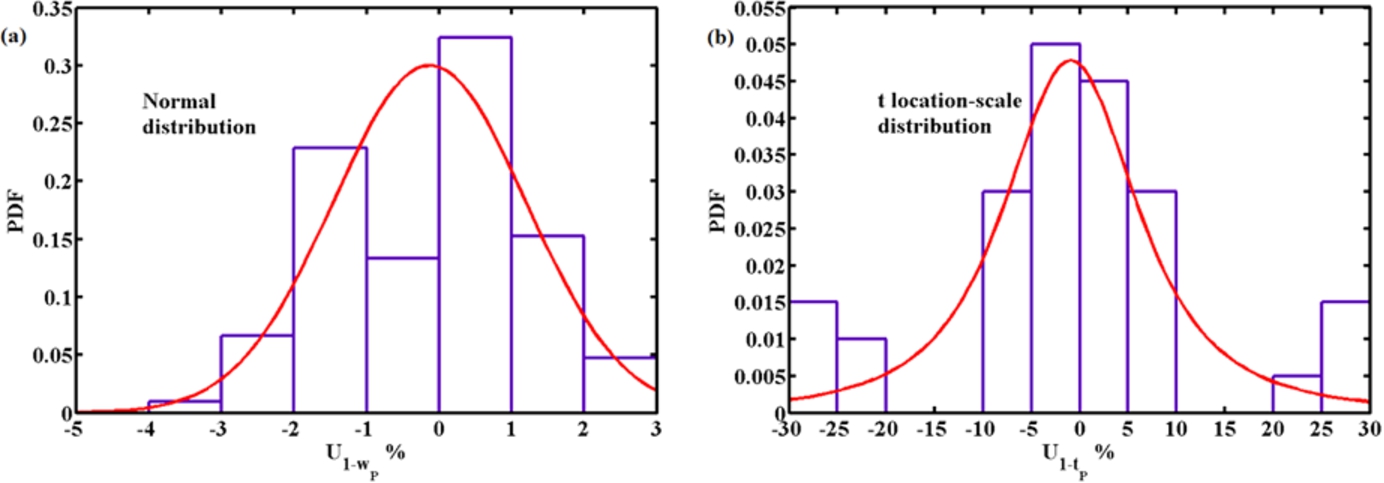
Probability distribution of mathematical modeling uncertainty in effective wake and thrust deduction fraction. Sample size is 50. (a) normal, , and (b) t location-scale, , , . (Colors are visible in the online version of the article; http://dx.doi.org/10.3233/ISP-150117.)
Comparison of mathematical predictions and test data of propeller thrust and torque. (Colors are visible in the online version of the article; http://dx.doi.org/10.3233/ISP-150117.)
Comparison of mathematical model simulation results of full-scale 20° zigzag maneuver at propeller revolution and free run experimental data of MARIN at . (Colors are visible in the online version of the article; http://dx.doi.org/10.3233/ISP-150117.)
Comparison of ship’s longitudinal speed and roll angle time series during 20° zigzag maneuver at with different twin-rudder conditions. Powering: constant torque. (Colors are visible in the online version of the article; http://dx.doi.org/10.3233/ISP-150117.)
Comparison of ship’s propeller revolution and main engine power during 20° zigzag maneuver at different twin-rudder conditions. Powering: constant torque. (Colors are visible in the online version of the article; http://dx.doi.org/10.3233/ISP-150117.)
Probability distribution of port and starboard propeller revolution during full-scale simulation of 20° zigzag maneuver at and , powering: constant torque (upper half) and gas turbine (lower half). Sample size is 105. (Colors are visible in the online version of the article; http://dx.doi.org/10.3233/ISP-150117.)
Probability distribution of power of port and starboard prime mover during full-scale simulation of 20° zigzag maneuver at and , powering: constant torque (upper half) and gas turbine (lower half). Sample size is 105. (Colors are visible in the online version of the article; http://dx.doi.org/10.3233/ISP-150117.)
Probability distribution of port and starboard rudder torque during full-scale simulation of 20° zigzag maneuver at and , powering: constant torque (upper half) and gas turbine (lower half). Sample size is 105. (Colors are visible in the online version of the article; http://dx.doi.org/10.3233/ISP-150117.)
Footnotes
References
1.
M.A.Abkowitz, Lectures on ship hydrodynamics – Steering and manoeuverability, 1964, No. HY-5.
2.
AIAA, Assessment of experimental uncertainty with application to wind tunnel testing, AIAA Standard S-071A-1999, Washington, DC.
3.
J.V.Amerongen, P.G.M.Van Der Klugt and H.R.Van Nauta Lemke, Roll stabilization of ships by means of the rudder, in: Proceedings of the Third Yale Workshop on Applications of Adaptive Systems Theory, New Haven, CT, 1983, pp. 19–26.
4.
ASME, Test uncertainty: Instruments and apparatus, PTC 19.1-1998, 1998.
5.
L.Benedetti, B.Bouscasse, R.Broglia, L.Fabbri, F.L.Gala and C.Lugni, PMM Model Test with DDG51 Including Uncertainty Analysis, INSEAN, Italy, 2004.
6.
P.M.Carrica, F.Ismail, M.Hyman, S.Bhushan and F.Stern, Turn and zigzag maneuvers of a surface combatant using a URANS approach with dynamic overset grids, Journal of Marine Science and Technology18(2) (2013), 166–181.
7.
A.Coraddu, G.Dubbioso, S.Mauro and M.Viviani, Experimental investigation of asymmetrical propeller behavior of twin screw ships during maneuvers, in: Proceedings of the International Conference on Marine Simulation and Ship Maneuverability MARSIM2012, Singapore, 2012.
8.
A.K.Dash and V.Nagarajan, A stochastic response surface approach for uncertainty propagation in ship maneuvering, International Shipbuilding Progress61(3-4) (2014), 129–161.
9.
K.S.M.Davidson and L.I.Schiff, Turning and course keeping qualities, Trans. SNAME54 (1946).
10.
Det Norske Veritas, Steering gear, in: Rules for Classification of Ships/High Speed, Light Craft and Naval Surface Craft, 2005, Part 4, Chapter 14.
11.
H.Eda, Maneuvering performance of high-speed ships with effect of roll motion, Ocean Engineering7(3) (1980), 379–397.
12.
R.G.Ghanem and P.D.Spanos, Stochastic Finite Element: A Spectral Approach, Revised Version, Dover Publication, Mineola, NY, 2003.
13.
J.M.Hammersley and D.C.Handscomb, Monte Carlo Methods, Vol. 1, Methuen, London, 1964.
K.Hasegawa, V.Nagarajan and D.H.Kang, Performance evaluation of Schilling rudder and mariner rudder for pure car carriers (PCC) under wind condition, in: MARSIM 2006, MIWB, Terschelling, The Netherlands, 26–29 June 2006, 2006.
16.
S.S.Isukapalli, An uncertainty analysis of transport transformation models, PhD thesis, The State University of New, Jersey, New Brunswick, NJ, 1999.
17.
ITTC, Uncertainty analysis in EFD, uncertainty analysis methodology 4.9-03-01-01, in: Proceedings of the 22nd International Towing Tank Conference, Seoul, Korea/Beijing, China, 1999.
18.
S.Khanfir, K.Hasegawa, V.Nagarajan, K.Shouji and S.K.Lee, Manoeuvring characteristics of twin-rudder systems: Rudder–hull interaction effect on the manoeuvrability of twin-rudder ships, Journal of Marine Science and Technology16(4) (2011), 472–490.
19.
H.J.Kim, S.H.Kim, J.K.Oh and D.W.Seo, A proposal on standard rudder device design procedure by investigation of rudder design process at major Korean shipyards, Journal of Marine Science and Technology20(4) (2012), 450–458.
20.
S.K.Lee and M.Fujino, Assessment of a mathematical model for the maneuvering motion of a twin propeller twin rudder ship, International Shipbuilding Progress50(1-2) (2003), 109–123.
21.
D.Q.Li, Y.Chen, W.Lu and C.Zhou, Stochastic response surface method for reliability analysis of rock slopes involving correlated non-normal variables, Computers and Geotechnics38 (2011), 58–68.
22.
J.Longo and F.Stern, Uncertainty assessment for towing tank tests with example for surface combatant DTMB model 5415, Journal of Ship Research49(1) (2005), 55–68.
23.
R.Mandal and Y.Kawamura, Stochastic formulation of structural response of steel plates with random initial distortions: An intrusive formulation using polynomial chaos expansions, Journal of the Japan Society of Naval Architects and Ocean Engineers19 (2014), 187–196.
24.
M.Mitchell and J.H.Holland, When will a genetic algorithm outperform hill-climbing?, in: Proceedings of the 5th International Conference on Genetic Algorithms, 1993.
25.
D.C.Montgomery and G.C.Runger, Applied Statistics and Probability for Engineers, John Wiley & Sons, 2010.
26.
C.J.Rubiset al., Acceleration and steady-state propulsion dynamics of a gas turbine ship with controllable-pitch propeller, Trans. SNAME80 (1972), 329–360.
27.
P.J.M.Schulten, The interaction between diesel engines, ship and propellers during manoeuvring, PhD thesis, Delft University of Technology, 2005.
28.
C.D.Simonsen, PMM Model Test with DDG51 Including Uncertainty Analysis, FORCE Technology, Denmark, 2004.
29.
K.H.Son and K.Nomoto, On the coupled motion of steering and rolling of a high-speed container ship, Naval Architecture and Ocean Engineering20 (1982), 73–83.
30.
F.Sternet al., Lessons learnt from the workshop on verification and validation of ship manoeuvring simulation methods – SIMMAN 2008, in: Proceedings of the International Conference on Marine Simulation and Ship Maneuverability, Panama City, Panama, 2009.
31.
J.Strøm-Tejsen and M.S.Chislett, A model testing technique and method of analysis for the prediction of steering and manoeuvring qualities of surface vessels, in: Sixth Symposium on Naval Hydrodynamics, 1966.
32.
S.Toxopeus, F.V.Walree and R.Hallmann, Manoeuvring and seakeeping tests for 5415M, MP-AVT-189-07, in: NATO AVT-189 Specialists Meeting on “Assessment of Stability and Control Prediction Methods for NATO Air and Sea Vehicles”, Portsdown-West, UK, 2011.
33.
S.L.Toxopeus and R.Hallmann, Validation and extension of the rotating arm functionality in the seakeeping and manoeuvring basin, Report No. 21569-1-DT/SMB, MARIN, The Netherlands, 2007.
34.
M.Ueno, Y.Yoshimura, Y.Tsukada and H.Miyazaki, Circular motion tests and uncertainty analysis for ship maneuverability, Journal of Marine Science and Technology14(4) (2009), 469–484.
35.
US Navy Combatant, DTMB 5415, available at: http://www.simman2008.dk/5415/5415_geometry.htm.
36.
R.V.Wilson, P.M.Carrica and F.Stern, Unsteady RANS method for ship motions with application to roll for a surface combatant, Computers & Fluids35(5) (2006), 501–524.
37.
H.Yoon, Phase-averaged stereo-PIV flow field and force/moment/motion measurements for surface combatant in PMM maneuvers, PhD thesis, University of Iowa, USA, 2009.