Estimation of hydrodynamic forces and motion of ships with steady forward speed

Abstract

The growing number of large ships demands predicting their optimum performance with respect to travel time, fuel efficiency and the safety of cargo and personnel in specified shipping routes. This can be achieved using efficient and easy to use numerical tools capable of predicting hydrodynamic loads on floating vessels with steady forward speed and solving their motion response in various wave conditions. A three-dimensional potential theory based code using the Green function method is developed with consideration of forward speed effects. The generalized coordinate system is used to allow motion response calculations with respect to any desired body coordinate system and a common quadrilateral meshing format. The formulation and calculation of added mass and damping coefficients at zero and infinite frequency in forward speed case has been also provided.

A number of structures including simple geometries and full ship hull forms have been analyzed and validated against published theoretical, numerical and experimental results. The comparison results are found to be in excellent agreement. The theoretical formulation, numerical implementation and result comparisons are presented here.

Keywords

Forward speed potential theory 3D panel method Green function

Nomenclature

ship forward speed

wave heading

wave amplitude

wave number

ω_{I}

incident wave frequency

ω_{e}

encounter wave frequency

ϕ_{I}

incident wave potential

ϕ_{s}

steady translation potential

ϕ_{D}

diffraction wave potential

ϕ_{j}

radiation potential due to unit motion in jth direction

η_{j}

jth vessel motion amplitude

acceleration due to gravity

m_{j}

gradient of the forward speed potential

Green function

A_{j k}

added mass coefficient

B_{j k}

radiation damping coefficient

M_{j k}

vessel mass matrix

C_{j k}

hydrostatic stiffness coefficient

F^{I}

Froude Krylov force

F^{D}

diffraction force

\vec{n}

unit normal pointing outward from the hull surface

hydrodynamic pressure on hull

source strength

Δ S_{j}

surface area of jth panel

1. Introduction

Potential theory methods have been in development for applications in aerodynamic and hydrodynamic problems for many decades. The mathematical derivation of the results using the fundamental laws of fluid mechanics has attracted researchers from around the world. Also the marine industries including navy, commercial ship building and the offshore oil and gas industries are currently using different seakeeping computer programs based on these theories for the design and operation of marine vehicles and structures.

The idea of representing irregular ocean waves as a superposition of many linear sinusoidal waves was first proposed by St. Denis and Pierson [48]. This opened the door for the development of both experimental and theoretical techniques to predict vessel response in random waves. Linear two-dimensional strip theories for seakeeping analysis were the most popular ones before the revolution in computing technologies. The widespread availability of high computational power has allowed the development of three-dimensional linear theories. Nonlinearities resulting from high seas have also been considered and later incorporated in both strip theory and three-dimensional panel methods.

The first strip theory for heave and pitch motions of ships in head seas was given by Korvin-Kroukovsky and Jacobs [27]. This was then refined by Gerritsma and Beukelman [10]. However, the most popular strip theory method is the one by Salvesen et al. [42] known as the STF method. In that work, the authors presented a complete linear potential theory considering forward speed of the vessel initially without any strip theory assumptions and then they applied strip theory to obtain the final results. The authors also mention that the theory presented is exact for the zero speed case within the assumptions of linear potential theory which allows analysis of non-slender bodies such as offshore platforms. The strip theory assumption restricts the use of these methods to slender bodies and only for the high frequency range and for low Froude numbers.

For higher sea states and Froude number greater than 0.4, the nonlinear effects may become important. The nonlinear strip theory methods tries to capture these through instantaneous wave elevation at every ship section [39].

One of the limitations of the strip theory method is that it is only valid for the high encounter frequency range. Newman [36] developed a method and then Newman and Sclavounos [38] modified the same to solve the seakeeping problem for different frequency range using near and far field methods and then joined them both to give a unified solution.

The era of the three-dimensional methods began when Hess and Smith [17] first introduced flow calculation about arbitrary, non-lifting, three-dimensional bodies using Rankine sources. Later, Hess and Wilcox [18] developed a computer program which included the previous method along with an undisturbed free surface by introducing a system of image sources. The Rankine source method have been used for solving ship motions problems in both the frequency domain [34] and the time domain [35]. The main difference between the Rankine source method and the 3D Green function method is that the Rankine sources do not satisfy the free surface boundary condition, and hence require panel discretization of the free surface around the floating body. This significantly increases the total number of panels in the computation.

The use of Green functions to represent the source potential in solving wave loads on floating offshore structures in the frequency domain was first introduced by Garrison [9]. This method became popular among many researchers and engineers as seen in [1,3,20,37,40,49], who have worked extensively in developing efficient methods to numerically evaluate the Green function. Efforts have been also made in developing a time-domain 3D Green function as well [2,31]. The strength of this method is that the Green function satisfies the free surface boundary conditions, and hence only the submerged part of the hull needs to be discretized. The lower number of panels improves calculation speed. However, it should be noted that the evaluation of the Green function is more time consuming compared to simple Rankine sources.

Even though the frequency domain potential theory and 3D panel method techniques have been around for a couple of decades and have been studied by many researchers, it is still a challenging task to implement them in a numerical code. Recent developments includes the panel free method using NURBS surface and potential theory based code presented by Qiu and Peng [41]. Kjellberg et al. [26] attempts to couple boundary element methods with a semi-Lagrangian free surface model to incorporate all nonlinearities of potential flow methods. Kashiwagi and Wang [24] shows a method to remove the moderate forward speed restriction in potential theory codes. A number of codes based on time-domain potential theory has been also developed of which the most recent is found in [15]. In order to focus this article in frequency domain, a complete literature review of the time-domain methods is not presented here.

It was found that some existing commercially available computer programs impose constraints such as resolution or total number of frequencies for which analysis can be performed or the number of bodies for which full QTF’s can be calculated [14]. In order to overcome these difficulties an in-house program called MDLHydroD has been developed. McTaggart [32] gives a concise guideline on implementing the 3D method and the work of Filkovic [7] provides a method for panel discretization. The derivation of forces and motions given by Salvesen et al. [42] using potential flow is also valid for 3D methods as well and therefore used here to obtain the final results. It is important to understand all the assumptions made in developing these theories and intricacies involved in implementation of the code. Any further development towards analysis of more complicated problems such as estimation of parametric roll, optimization of hull, multi-body interaction or coupled hydrodynamics with mooring and risers relies on accurate estimation of the linear assumptions. The following sections give details of hydrodynamic problem formulation, numerical implementation and comparison of results.

Fig. 1.

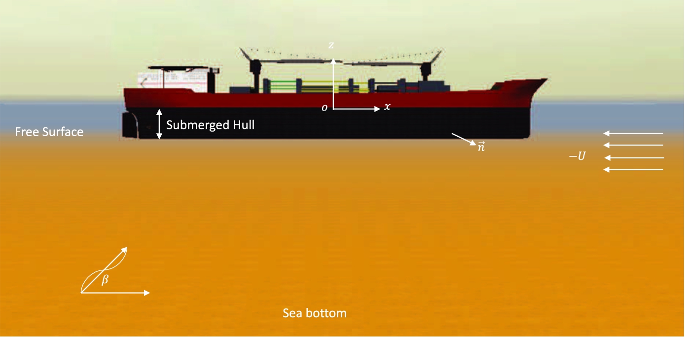
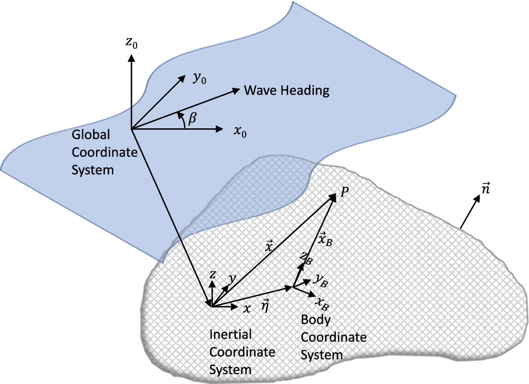
Definition sketch. (Colors are visible in the online version of the article; https://dx-doi-org.web.bisu.edu.cn/10.3233/ISP-150118.)

Fig. 2.

Generalized coordinate system. (Colors are visible in the online version of the article; https://dx-doi-org.web.bisu.edu.cn/10.3233/ISP-150118.)

2. Definition of the hydrodynamic problem

A ship moving with a steady forward speed U in deep water with regular waves of wave amplitude A and incident frequency $ω_{I}$ traveling at an angle β is considered (see Fig. 1). A generalized coordinate system is defined with an earth fixed global coordinate system, an inertial coordinate system translating with body and a body fixed coordinate system (see Fig. 2). The translating reference frame allows us to formulate the vessel response in six degree of freedom due to incident waves and steady current of speed U in $- x$ direction which is equivalent to forward speed with respect to a fixed reference frame. A linear boundary value problem can be defined under the small amplitude wave assumption to determine the velocity potential of the flow field. A complex velocity potential can be defined under the assumption of inviscid, incompressible and irrotational fluid as: $\begin{array}{rcl} Φ (\vec{x}, t) & = & [- U x + ϕ_{S} (\vec{x})] \\ (2.1) & + [ϕ_{I} (\vec{x}, β, ω_{I}) + ϕ_{D} (\vec{x}, β, ω_{I}) + \sum_{j = 1}^{6} η_{j} ϕ_{j} (\vec{x}, U, ω_{e})] e^{i ω_{e} t}, \end{array}$ where $ω_{e}$ denotes encounter frequency; $ϕ_{S}$ represents the perturbation potential due to steady translation; $ϕ_{I}$ is the incident wave potential; $ϕ_{D}$ is the diffracted wave potential; $ϕ_{j}$ and $η_{j}$ are the radiation potential due to unit motion and vessel motion amplitude respectively in the jth direction. The encounter frequency is expressed in terms of the incident wave frequency as: $\begin{matrix} (2.2) & ω_{e} = ω_{I} - \frac{ω_{I}^{2}}{g} U cos β . \end{matrix}$ The perturbation potential $ϕ_{S}$ is ignored due to the complexity of derivation and its relatively insignificant effect at moderate ship speed. The remaining incident wave potential $ϕ_{I}$ , diffraction potential $ϕ_{D}$ and radiation potential $ϕ_{j}$ are determined by solving the following boundary value problem:

The velocity potentials satisfy the Laplace equation in the fluid domain: $\begin{matrix} (2.3) & \nabla^{2} (ϕ_{I}, ϕ_{D}, ϕ_{j}) = 0 . \end{matrix}$ The boundary conditions to be satisfied by the potential functions are:

Free-surface boundary condition: $\begin{matrix} (2.4) & [{(i ω_{e} - U \frac{\partial}{\partial x})}^{2} + g \frac{\partial}{\partial z}] (ϕ_{I}, ϕ_{D}, ϕ_{j}) = 0 on z = 0 . \end{matrix}$

The bottom boundary condition $\begin{matrix} (2.5) & \frac{\partial}{\partial z} (ϕ_{I}, ϕ_{D}, ϕ_{j}) = 0 on z \to - \infty . \end{matrix}$

The Sommerfeld radiation condition: The waves generated by the oscillating body must radiate outward from the body [33] $\begin{matrix} (2.6) & lim_{k r \to \infty} \sqrt{k r} (\frac{\partial}{\partial r} - i k) (ϕ - ϕ_{I}) = 0 . \end{matrix}$

The body surface boundary condition: $\begin{matrix} (2.7) & \frac{\partial ϕ_{j}}{\partial n} = i ω_{e} n_{j} + U m_{j} on S \end{matrix}$ and $\begin{matrix} (2.8) & \frac{\partial ϕ_{I}}{\partial n} + \frac{\partial ϕ_{D}}{\partial n} = 0 on S, \end{matrix}$ where $\vec{n} = (n_{1}, n_{2}, n_{3})$ is the unit normal pointing outward from the hull surface and $(n_{4}, n_{5}, n_{6}) = \vec{r} \times \vec{n}$ , $\vec{r}$ being the position vector of a point on the surface.

The well-known m-terms (

m_{j}

) are the components of the generalized vector involving the gradient of the forward speed potential,

\begin{matrix} (2.9) & \begin{matrix} (m_{1}, m_{2}, m_{3}) = (\vec{n} \cdot \nabla) \nabla Φ, \\ (m_{4}, m_{5}, m_{6}) = (\vec{n} \cdot \nabla) (\vec{r} \times \nabla Φ) \end{matrix} \end{matrix}

which are simplified to be

\begin{matrix} (2.10) & m_{j} \approx (0, 0, 0, 0, n_{3}, - n_{2}) . \end{matrix}

The linear incident wave potential satisfying the above boundary conditions is given by:

\begin{matrix} (2.11) & ϕ_{I} = \frac{i g A}{ω_{I}} e^{- i k_{I} (x cos β + y sin β)} e^{k z} . \end{matrix}

It has been shown in [42] that the radiation potential in the forward speed case can be represented in terms of the zero speed potentials as:

\begin{matrix} (2.12) & \begin{matrix} ϕ_{j} = ϕ_{j}^{0} for j = 1, 2, 3, 4, \\ ϕ_{5} = ϕ_{5}^{0} + \frac{U}{i ω_{e}} ϕ_{3}^{0}, \\ ϕ_{6} = ϕ_{6}^{0} - \frac{U}{i ω_{e}} ϕ_{2}^{0} . \end{matrix} \end{matrix}

Salvesen et al. [42] also shows by using Greens identity and a variant of Stokes theorem that the whole boundary value problem in forward speed condition can be solved by obtaining the zero speed condition results and modifying them appropriately. The zero speed boundary value problem can be solved using the method introduced by Garrison [9] based on a free surface Green function.

3. Numerical solution

3.1. Source distribution method

The complex potential on the submerged surface of the vessel is the key to solving the hydrodynamic problem. It will be shown that once the potential is known, all the hydrodynamic coefficients required to obtain the vessel response, i.e. added mass, damping and excitation forces can be calculated.

To obtain a numerical solution, sources of unknown strengths are distributed on the surface of the body. The velocity potential function can be written in terms of the unknown source strengths as: $\begin{matrix} (3.1) & ϕ^{0} (\vec{x}) = \frac{1}{4 π} \int_{S} σ ({\vec{x}}_{s}) G (\vec{x}, {\vec{x}}_{s}) d s, \end{matrix}$ where $\vec{x}$ denotes the point where the potential is being evaluated due to a source at ${\vec{x}}_{s}$ on the body surface S. The superscript on $ϕ^{0}$ denotes the potential for the zero speed case. $σ ({\vec{x}}_{s})$ denotes the source strength which is unknown and needs to be calculated by solving the boundary value problem. The function $G (\vec{x}, {\vec{x}}_{s})$ is a Green function which satisfies the Laplace equation, the free surface, radiation and bottom boundary conditions. The derivation of the potential using the Green function can be found in [9]. However, for numerical implementation, the Green function developed by Telste and Noblesse [49] is used.

The unknown source strengths are calculated using the radiation and diffraction body boundary conditions separately by substituting Eq. (3.1) into Eqs (2.7) and (2.8). The resulting integral equation is: $\begin{matrix} (3.2) & - \frac{1}{2} σ_{i} + \frac{1}{4 π} \int_{S} σ ({\vec{x}}_{s}) \frac{\partial G}{\partial n} (\vec{x}, {\vec{x}}_{s}) d s = v_{n_{i}}, \end{matrix}$ where $\begin{array}{l} v_{n} & = i ω_{e} n_{j} (radiation potential) \\ (3.3) & = - \frac{\partial ϕ_{I}^{0}}{\partial n} (diffraction potential) . \end{array}$ Quadrilateral panels are used to discretize the submerged hull surface. The surface integral may be written as the sum of the integrals over N panels (excluding the ith panel) of area $Δ S_{j}$ . As an approximation, the source strength $σ ({\vec{x}}_{s})$ may be taken as constant over each panel. The resulting discretized equation is: $\begin{matrix} (3.4) & - \frac{1}{2} σ_{i} + \frac{1}{2} \sum_{j = 1}^{N} α_{i j} σ_{j} = v_{n_{i}} (i = 1, \dots, N), \end{matrix}$ where $\begin{matrix} (3.5) & α_{i j} = \frac{1}{2 π} \int_{Δ S_{j}} \frac{\partial G}{\partial n} (\vec{x}, {\vec{x}}_{s}) d s . \end{matrix}$ The potential $ϕ^{0}$ at the center of each panel can be calculated using Eq. (3.1) as: $\begin{matrix} (3.6) & ϕ_{i}^{0} = \sum_{j = 1}^{N} β_{i j} σ_{j}, \end{matrix}$ where $\begin{matrix} (3.7) & β_{i j} = \frac{1}{4 π} \int_{Δ S_{j}} G (\vec{x}, {\vec{x}}_{s}) d s . \end{matrix}$

The evaluation of matrix α in Eq. (3.5) and β in Eq. (3.7) requires integration of the Green function and its derivatives over the panel surface. Katz and Plotkin [25] give an analytical expression for integrating the singular but frequency independent part of the Green function, $\int_{S_{j}} (\frac{1}{r}) d s$ and Hess and Smith [17] gives analytical expression for integrating the derivatives of the frequency independent part of the Green function $\int_{Δ S_{j}} \frac{\partial}{\partial n} (\frac{1}{r}) d s$ . The same analytical expressions can also be used to calculate the image source portion of the Green function $\int_{S_{j}} (\frac{1}{r^{'}}) d s$ and $\int_{S_{j}} \frac{\partial}{\partial n} (\frac{1}{r^{'}}) d s$ .

The integration of the frequency dependent term $\int_{S_{j}} {\tilde{G}}_{0} (\vec{x}, {\vec{x}}_{s}) d s$ and its derivative $\int_{S_{j}} \frac{\partial {\tilde{G}}_{0}}{\partial n} (\vec{x}, {\vec{x}}_{s}) d s$ can be obtained in multiple ways. A Gauss quadrature method may be applied for higher accuracy. However, these terms are regular throughout the fluid domain and oscillate approximately with the wave length [9]. In practice,the panel size is generally small compared to the wave length and hence ${\tilde{G}}_{0} (\vec{x}, {\vec{x}}_{s})$ can be considered constant over the panel surface $Δ S_{j}$ . Hence, a convenient approximation to the integral is to evaluate the integrand at the centroid of the panel and multiply it by $Δ S_{j}$ .

The collection of equations required for calculation of panel properties such as the normal vector, panel area and finally evaluation of the α and β matrices are given in [11,13] in further detail.

3.2. Hydrodynamic coefficients

Once the velocity potential is obtained at each panel, the hydrodynamic coefficients can be easily solved by calculating the pressure on the hull and integrating the pressure on the hull surface. The pressure on the hull can be found using the Bernoulli’s equation: $\begin{matrix} (3.8) & P = \frac{1}{2} ρ U^{2} - ρ \frac{\partial Φ}{\partial t} - \frac{1}{2} ρ | \nabla Φ |^{2} - ρ g z \end{matrix}$ and the hydrostatic and hydrodynamic force can be calculated by: $\begin{matrix} (3.9) & F_{H_{j}} = - \int_{S} P n_{j} d s, j = 1, 2, \dots, 6 . \end{matrix}$ The zero speed hydrodynamic coefficients are given by: $\begin{array}{rcl} (3.10) & A_{j k}^{0} = - \frac{ρ}{ω_{e}} \int_{S} Im (ϕ_{k}) n_{j} d s, \\ (3.11) & B_{j k}^{0} = - ρ \int_{S} Re (ϕ_{k}) n_{j} d s \end{array}$ with speed correction terms given as: $\begin{matrix} (3.12) & \begin{matrix} A_{15} = A_{15}^{0} - \frac{U}{ω_{e}^{2}} B_{13}^{0}, & A_{26} = A_{26}^{0} + \frac{U}{ω_{e}^{2}} B_{22}^{0}, & A_{55} = A_{55}^{0} + \frac{U^{2}}{ω_{e}^{2}} A_{33}^{0}, \\ B_{15} = B_{15}^{0} + U A_{13}^{0}, & B_{26} = B_{26}^{0} - U A_{22}^{0}, & B_{55} = B_{55}^{0} + \frac{U^{2}}{ω_{e}^{2}} B_{33}^{0}, \\ A_{51} = A_{51}^{0} + \frac{U}{ω_{e}^{2}} B_{31}^{0}, & A_{62} = A_{62}^{0} - \frac{U}{ω_{e}^{2}} B_{22}^{0}, & A_{66} = A_{66}^{0} + \frac{U^{2}}{ω_{e}^{2}} A_{22}^{0}, \\ B_{51} = B_{51}^{0} - U A_{31}^{0}, & B_{62} = B_{62}^{0} + U A_{22}^{0}, & B_{66} = B_{66}^{0} + \frac{U^{2}}{ω_{e}^{2}} B_{22}^{0}, \\ A_{35} = A_{35}^{0} - \frac{U}{ω_{e}^{2}} B_{33}^{0}, & A_{46} = A_{46}^{0} + \frac{U}{ω_{e}^{2}} B_{24}^{0}, \\ B_{35} = B_{35}^{0} + U A_{33}^{0}, & B_{46} = B_{46}^{0} - U A_{24}^{0}, \\ A_{53} = A_{53}^{0} + \frac{U}{ω_{e}^{2}} B_{33}^{0}, & A_{64} = A_{64}^{0} - \frac{U}{ω_{e}^{2}} B_{24}^{0}, \\ B_{53} = B_{53}^{0} - U A_{33}^{0}, & B_{64} = B_{64}^{0} + U A_{24}^{0} . \end{matrix} \end{matrix}$

The incident wave excitation force also known as the Froude Krylov force is given by: $\begin{matrix} (3.13) & F_{I} = i ω_{I} ρ \int_{S} ϕ_{I} n_{j} d s \end{matrix}$ and the diffraction wave excitation force is $\begin{array}{l} F_{D} & = ρ \int_{S} (i ω_{e} n_{j} - U m_{j}) ϕ_{D} d s \\ = - ρ \int_{S} ϕ_{j}^{0} \frac{\partial ϕ_{I}}{\partial n} d s for j = 1, 2, 3, 4 \\ = - ρ \int_{S} ϕ_{j}^{0} \frac{\partial ϕ_{I}}{\partial n} d s + \frac{ρ U}{i ω_{e}} \int_{S} ϕ_{3}^{0} \frac{\partial ϕ_{I}}{\partial n} d s for j = 5 \\ (3.14) & = - ρ \int_{S} ϕ_{j}^{0} \frac{\partial ϕ_{I}}{\partial n} d s - \frac{ρ U}{i ω_{e}} \int_{S} ϕ_{2}^{0} \frac{\partial ϕ_{I}}{\partial n} d s for j = 6 . \end{array}$ The calculated added mass, damping and wave excitation forces are used to solve the equation of motion to get the vessel response $\begin{matrix} (3.15) & \sum_{k = 1}^{6} [- ω_{e}^{2} (M_{j k} + A_{j k}) + i ω_{e} B_{j k} + C_{j k}] η_{k} = F_{j}^{I} + F_{j}^{D}, j = 1, 2, \dots, 6, \end{matrix}$ where $M_{j k}$ is the mass matrix, $C_{j k}$ is the hydrostatic stiffness matrix and $η_{k}$ the vessel response in kth mode of motion.

3.3. Added mass and damping at zero and infinite frequency

The added mass and damping coefficients for the frequency limits $ω = 0$ and $ω \to \infty$ are important for calculating impulse response functions for time-domain analysis. The frequency domain approach described in previous section presents numerical limitations for high frequency oscillations based on panel size and requires modification in the potential theory formulation.

The time dependent velocity potential is represented as: $\begin{matrix} (3.16) & Φ = Real {ϕ e^{i ω_{e} t}} . \end{matrix}$ In the above equation, for zero and infinite frequency ϕ is replaced by: $\begin{matrix} (3.17) & ϕ = i ω_{e} ϕ^{'} . \end{matrix}$ The body boundary condition for radiation potential becomes: $\begin{matrix} (3.18) & \begin{matrix} \frac{\partial ϕ_{j}}{\partial n} = i ω_{e} n_{j}, \\ i ω_{e} \frac{\partial ϕ_{j}^{'}}{\partial n} = i ω_{e} n_{j}, \\ \frac{\partial ϕ_{j}^{'}}{\partial n} = n_{j} . \end{matrix} \end{matrix}$ The solution of $ϕ^{'}$ is obtained using the source distribution method. The governing equation for $ϕ^{'}$ is: $\begin{matrix} (3.19) & {\vec{\nabla}}^{2} ϕ_{j}^{'} = 0 . \end{matrix}$ The free surface boundary condition is given by: $\begin{matrix} (3.20) & \begin{matrix} \frac{\partial^{2} Φ}{\partial t^{2}} + g \frac{\partial Φ}{\partial z} = 0 at z = 0, \\ - ω_{e}^{2} ϕ + g \frac{\partial ϕ}{\partial z} = 0, \\ - ω_{e}^{2} ϕ^{'} + g \frac{\partial ϕ^{'}}{\partial z} = 0 . \end{matrix} \end{matrix}$ At low frequency limit $ω_{e} = 0$ , the free surface appears as a rigid boundary. This gives the free surface boundary condition as: $\begin{matrix} (3.21) & \frac{\partial ϕ^{'}}{\partial z} = 0 at z = 0 for ω_{e} = 0 . \end{matrix}$ At the high frequency limit $ω_{e} \to \infty$ , the free surface boundary condition becomes: $\begin{matrix} (3.22) & ϕ^{'} = 0 at z = 0 and ω_{e} \to \infty . \end{matrix}$ The Green function that satisfies the above governing equations are given by: $\begin{array}{l} (3.23) & G (\vec{x}, {\vec{x}}_{s}) = \frac{1}{r} + \frac{1}{r^{'}} for ω_{e} = 0, \\ (3.24) & G (\vec{x}, {\vec{x}}_{s}) = \frac{1}{r} - \frac{1}{r^{'}} for ω_{e} \to \infty . \end{array}$ The boundary condition for zero and infinite frequency are real numbers and the Green function is also a real number. This gives us a real $ϕ_{k}^{'}$ . Hence, $\begin{matrix} (3.25) & Im (ϕ_{k}^{'}) = 0 . \end{matrix}$

Substituting $ϕ_{k}^{'}$ in zero speed added mass (Eq. (3.10)) and damping (Eq. (3.11)) equation and using, we get: $\begin{matrix} (3.26) & \begin{matrix} A_{j k}^{0} = - \frac{ρ}{ω_{e}} \int_{S} Im (i ω_{e} ϕ_{k}^{'}) n_{j} d s = - ρ \int_{S} Re (ϕ_{k}^{'}) n_{j} d s, \\ B_{j k}^{0} = - ρ \int_{S} \underset{0}{\underset{︸}{Re (i ω_{e} ϕ_{k}^{'})}} n_{j} d s = 0 . \end{matrix} \end{matrix}$ We found that for zero speed ( $U = 0$ ), added mass coefficients are non-zero and damping coefficients are zero. For the forward speed case we use the added mass and damping modifications as explained in previous section. The terms that will get affected due to forward speed are listed below:

For both $ω = 0$ and $ω = \infty$ : $\begin{matrix} (3.27) & \begin{matrix} B_{15} = U A_{13}^{0}, & B_{35} = U A_{33}^{0}, & B_{26} = - U A_{22}^{0}, & B_{46} = - U A_{24}^{0}, \\ B_{51} = - U A_{31}^{0}, & B_{53} = - U A_{33}^{0}, & B_{62} = U A_{22}^{0}, & B_{64} = U A_{24}^{0} . \end{matrix} \end{matrix}$

For $ω \to \infty$ , the forward speed modification part becomes zero and hence: $\begin{matrix} (3.28) & \begin{matrix} A_{55} = A_{55}^{0}, & A_{66} = A_{66}^{0}, \\ B_{55} = B_{55}^{0}, & B_{66} = B_{66}^{0} . \end{matrix} \end{matrix}$

The added mass and damping coefficients $A_{55}$ , $B_{55}$ , $A_{66}$ , $B_{66}$ cannot be obtained for $ω = 0$ for the forward speed case. This however does not affect calculation of impulse response function by a large amount if the first non-zero frequency is chosen very close to zero i.e. $ω = 0.01$ . Figure 3 shows the heave added mass ( $A_{33}$ ) of a floating hemisphere at zero forward speed (a) and at $Fn = 0.16$ (b) for both zero and infinite frequency (infinite frequency value shown at the end point of the extended tail). The zero speed case has been validated against an industry standard computer program [29]. The validity of the forward speed case can be noticed easily at zero frequency as the curve is continuous and at infinite frequency the value is same as the zero speed infinite frequency value as expected.

Fig. 3.

Added mass ( $A_{33}$ ) of a floating hemisphere at zero forward speed (a) and at forward speed with $Fn = 0.16$ (b) showing results for zero and infinite frequency (extended tail). (Colors are visible in the online version of the article; https://dx-doi-org.web.bisu.edu.cn/10.3233/ISP-150118.)

The above mentioned numerical scheme is implemented in the code MDLHydroD written in FORTRAN programming language. All recent advancements in the potential theory field has been studied thoroughly during the development of the code. Keeping in mind the ease of use, the panel definition is obtained through commercial software [4] as a Geometric Data File format. This allows creating vessel geometry and studying its response about any point of origin on the hull easier and also encourage automated hull generation that can be used for hull form optimization purposes. Not requiring free surface discretization removes possible user error in deciding the size of the free surface domain and panelization errors near the hull waterline which may result in erroneous results. Using only the hull surface below mean waterline without surface discretization makes MDLHydroD robust, computationally efficient and useful for both manual and automatically generated hulls. However, this required using linearized free surface boundary condition which is a compromise as compared to Rankine source based codes with free surface panels. It must be recalled that the free surface non-linearities becomes significant beyond Froude number $Fn = 0.4$ and at high seas [6].

4. Results and comparison

The developed computer program MDLHydroD has been validated for a number of structures including simple geometries such as a floating hemisphere, box barge, spheroid and Wigley hulls as well as multiple ship forms and offshore platforms. The experimental and numerical results of Kashiwagi et al. [23] on a modified Wigley hull are compared for zero speed surge, heave and pitch motion responses.

The modified Wigley hull is represented mathematically as: $\begin{matrix} (4.1) & η = (1 - ζ^{2}) (1 - ξ^{2}) (1 + a_{2} ξ^{2} + a_{4} ξ^{4}) + ζ^{2} (1 - ζ^{8}) {(1 - ξ^{2})}^{4}, \end{matrix}$ where $ξ = x / (L / 2)$ , $η = y / (B / 2)$ and $ζ = z / T$ , with L, B and T the length, breadth and draft, respectively. $a_{2}$ and $a_{4}$ are bluntness coefficient and taken as $a_{2} = 0.6$ and $a_{4} = 1.0$ in the experimental model. The hull shape is relatively blunt and close to general ship forms. The discretized panel model and principal particulars of the hull are shown in Fig. 4 and Table 1. The experiments were conducted with model allowed to perform only surge, heave and pitch motion. Figures 5, 6 and 7 shows the motion amplitude and phase comparisons for the head sea condition which is in excellent agreement with experimental results and coincides with the 3D-HOBEM results. Further validations including hemisphere, cylinder, box barge, spar platform, TLP and Ro-Ro ship for zero forward speed case can be found in [11,13].

Fig. 4.

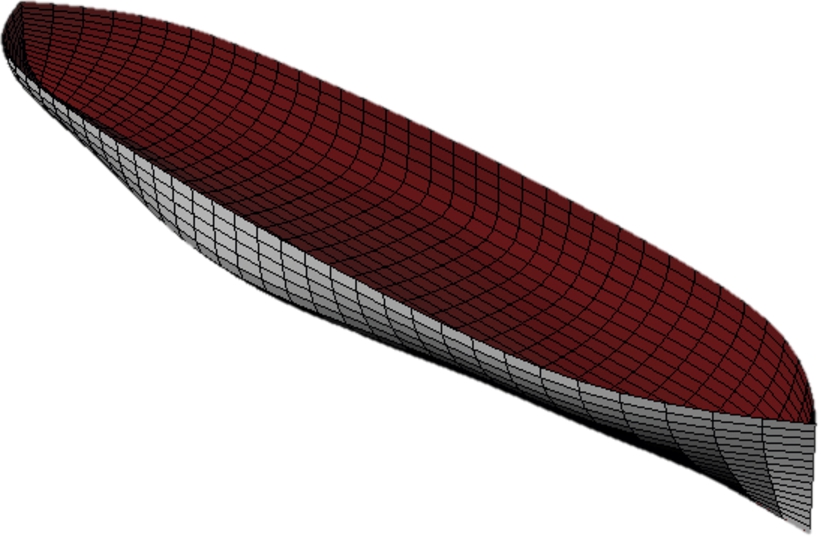
Panel model of modified Wigley I. (Colors are visible in the online version of the article; https://dx-doi-org.web.bisu.edu.cn/10.3233/ISP-150118.)

Table 1

Principal particulars of modified Wigley hull I

Principal particulars
Length (L)	2.5 m
Breadth (B)	0.5 m
Draft (T)	0.175 m
Displacement (Δ)	0.13877 m³
Radius of gyration ( $K_{y y} / L$ )	0.236
Center of gravity ( $OG$ )	0.031 m

Fig. 5.

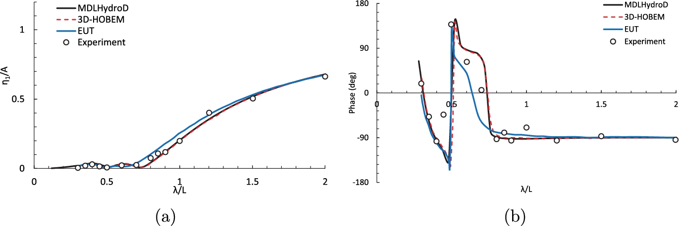
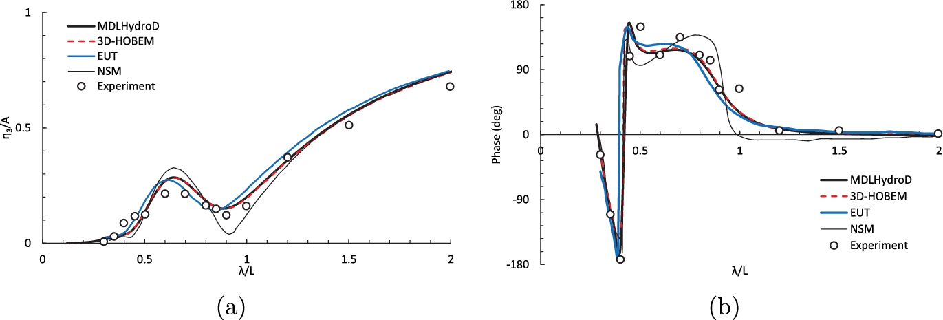
Surge motion amplitude (a) and phase (b) of the modified Wigley I model in head waves at zero forward speed. (Colors are visible in the online version of the article; https://dx-doi-org.web.bisu.edu.cn/10.3233/ISP-150118.)

Fig. 6.

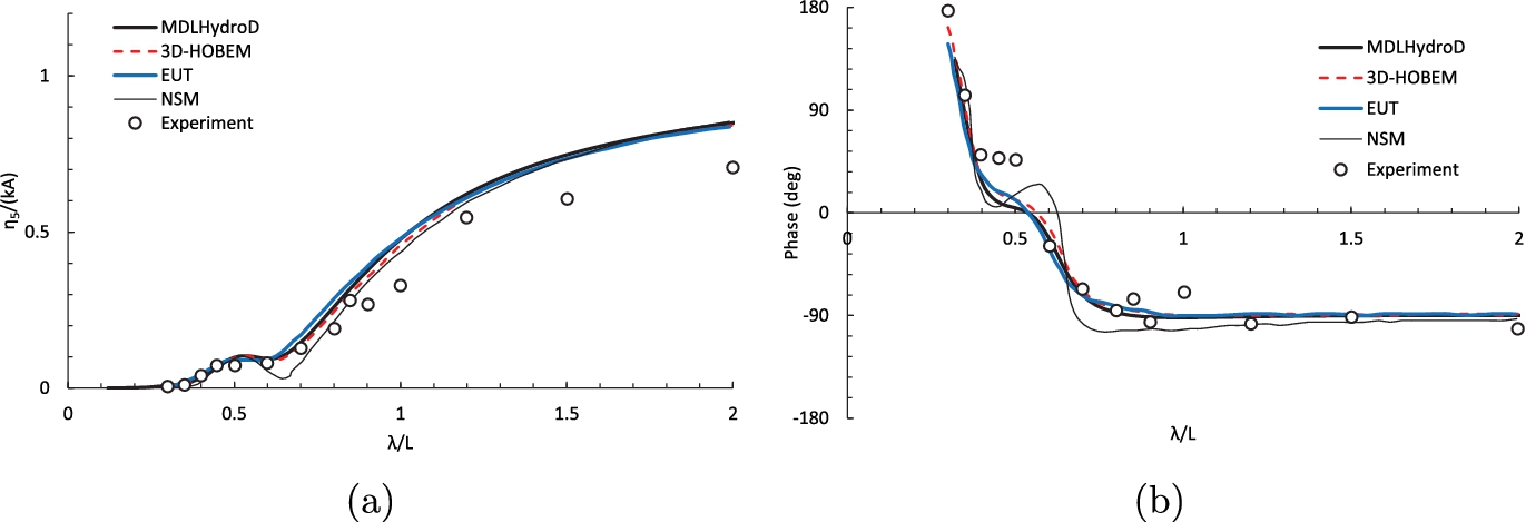
Heave motion amplitude (a) and phase (b) of the modified Wigley I model in head waves at zero forward speed. (Colors are visible in the online version of the article; https://dx-doi-org.web.bisu.edu.cn/10.3233/ISP-150118.)

Fig. 7.

Pitch motion amplitude (a) and phase (b) of the modified Wigley I in head sea at zero forward speed. (Colors are visible in the online version of the article; https://dx-doi-org.web.bisu.edu.cn/10.3233/ISP-150118.)

Fig. 8.

Panel model of modified Wigley II. (Colors are visible in the online version of the article; https://dx-doi-org.web.bisu.edu.cn/10.3233/ISP-150118.)

Table 2

Principal particulars of modified Wigley hull II

Principal particulars
Length (L)	2.0 m
Breadth (B)	0.3 m
Draft (T)	0.125 m
Displacement (Δ)	0.04197 m³
Radius of gyration ( $K_{y y} / L$ )	0.236
Center of gravity ( $OG$ )	0.0 m

Fig. 9.

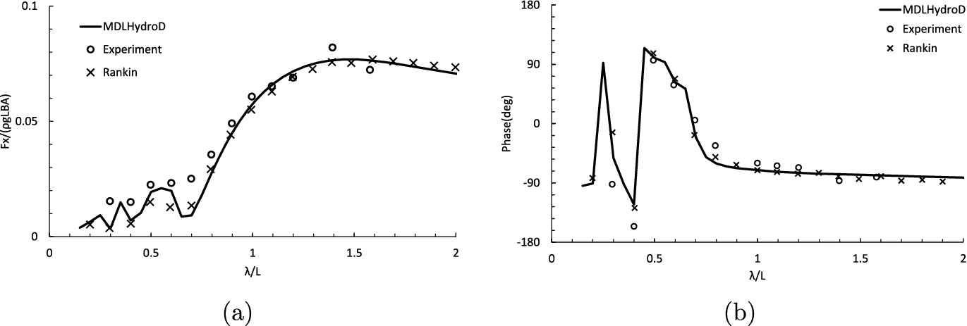
Surge excitation force amplitude (a) and phase (b) of the modified Wigley II in head wave with forward speed corresponding to $Fn = 0.2$ .

Fig. 10.

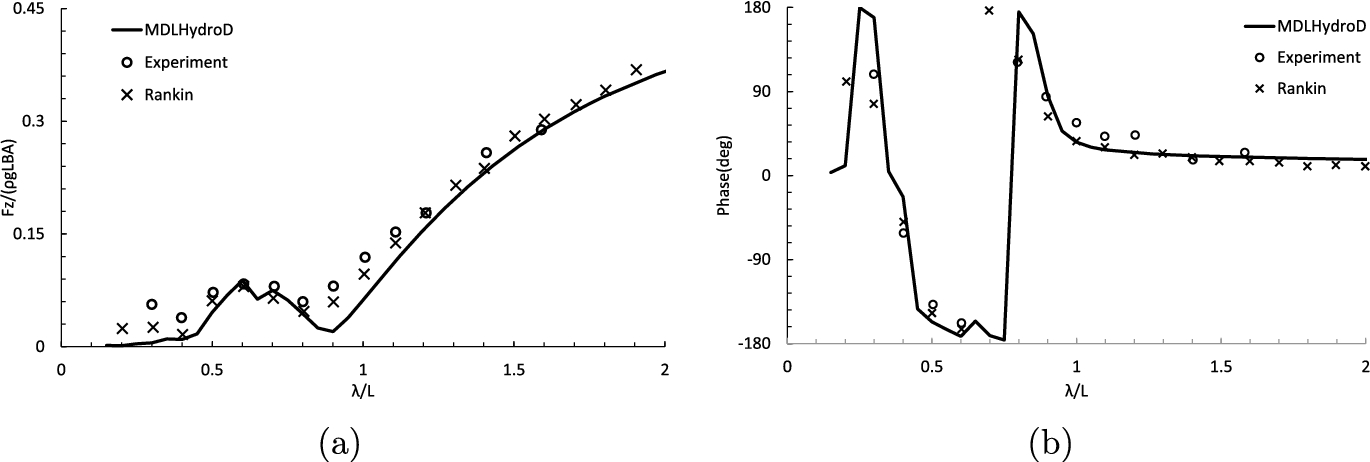
Heave excitation force amplitude (a) and phase (b) of the modified Wigley II in head wave with forward speed corresponding to $Fn = 0.2$ .

Fig. 11.

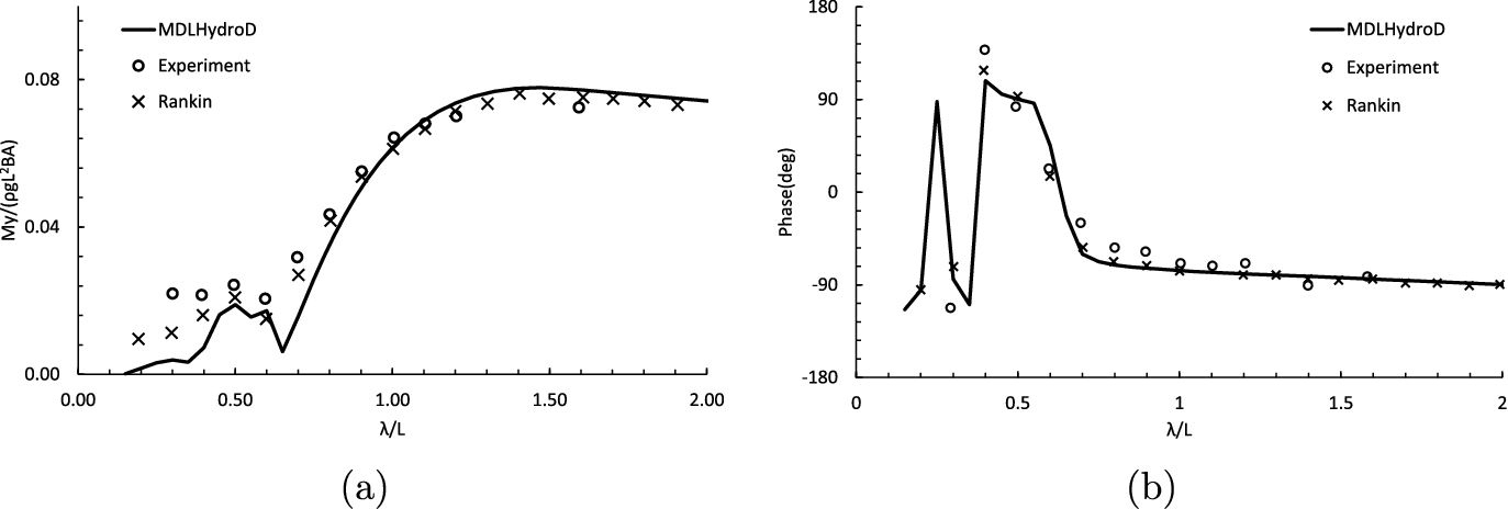
Pitch excitation force amplitude (a) and phase (b) of the modified Wigley II in head waves at forward speed corresponding to $Fn = 0.2$ .

Fig. 12.

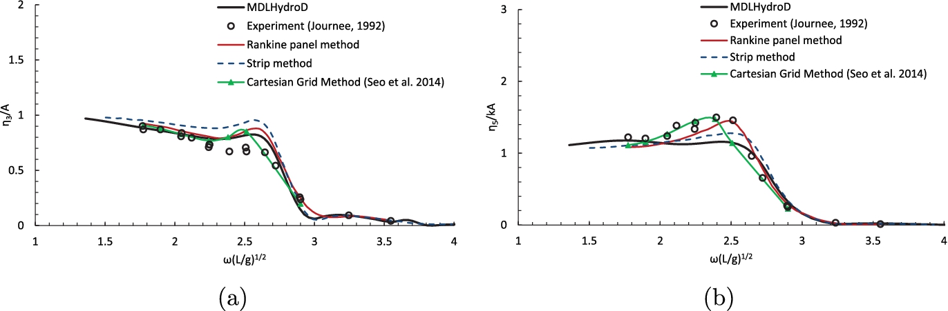
Heave (a) and pitch (b) motion amplitude of Wigley hull III in head wave at $Fn = 0.2$ . (Colors are visible in the online version of the article; https://dx-doi-org.web.bisu.edu.cn/10.3233/ISP-150118.)

Fig. 13.

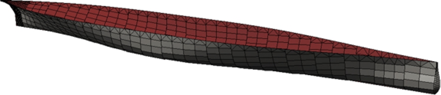
Panel model of KVLCC2. (Colors are visible in the online version of the article; https://dx-doi-org.web.bisu.edu.cn/10.3233/ISP-150118.)

Table 3

Principal particulars of KVLCC2

Principal particulars
Length (L)	320 m
Breadth (B)	58 m
Draft (T)	20.8 m
Displacement (Δ)	312,622 m³
LCG	11.1 m
GM	5.71 m

Fig. 14.

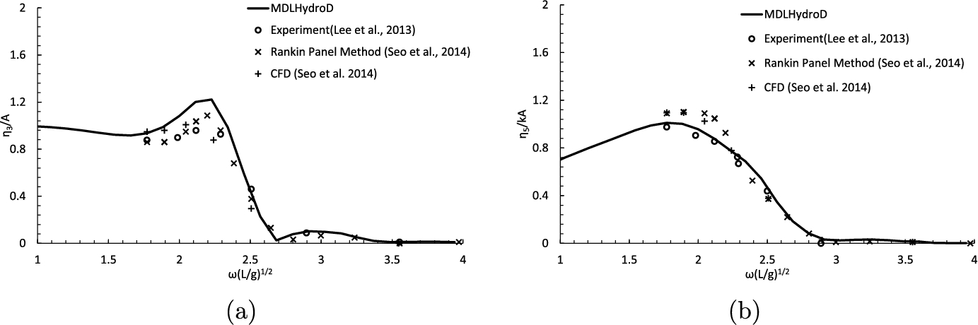
Heave (a) and pitch (b) motions of KVLCC2 in head wave at forward speed $Fn = 0.142$ .

Fig. 15.

Panel model of the S175 container ship. (Colors are visible in the online version of the article; https://dx-doi-org.web.bisu.edu.cn/10.3233/ISP-150118.)

Table 4

Principal particulars of S175

Principal particulars
Length between perpendiculars (L)	175 m
Breadth (B)	25.4 m
Height (H)	15.4 m
Design draught (T)	9.5 m
Displacement (Δ)	24,856 t
Vertical center of gravity (from baseline) ( $Z_{g}$ )	9.5 m
Roll radius of gyration ( $k_{x x}$ )	8.33 m
Pitch radius of gyration ( $k_{y y}$ )	42 m
Yaw radius of gyration ( $k_{z z}$ )	35.4 m

Another modified Wigley hull with the same mathematical hull surface description as Eq. (4.1) with, $a_{2} = 0.2$ , $a_{4} = 0$ , $L = 2.0 m$ , $B = 0.3 m$ , and $T = 0.125 m$ is studied by [16] for ships with forward speed. The experiments were performed on this model by Wakabayashi [50] for Froude number $Fn = U / \sqrt{g L} = 0.2$ in the head sea condition.

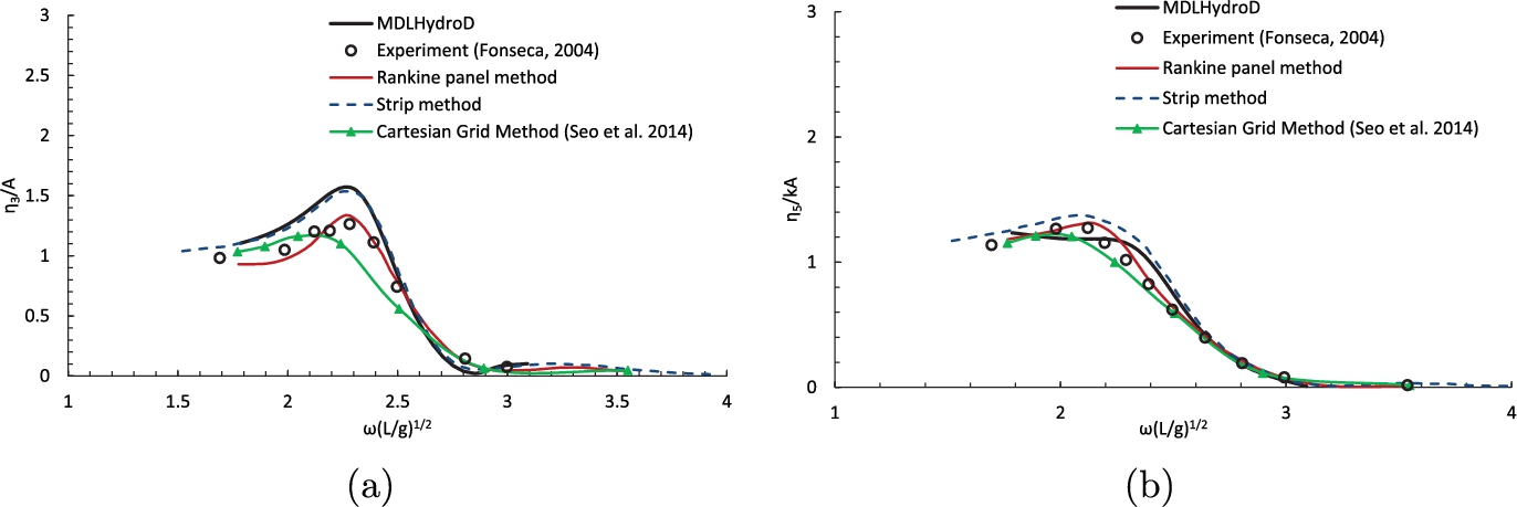
The comparison of wave exciting force amplitude and phase on the slender Wigley hull (Fig. 8, Table 2) at forward speed corresponding to $F n = 0.2$ are shown in Figs 9, 10 and 11. It can be seen that the presented numerical code is in good agreement with both experimental and Rankin method based results. The discrepancy between experimental results and the numerical code found near short wavelengths are expected as the panel size is relatively larger when short wavelengths are considered. The ideal panel size of the largest panel should be 1/8th of the wave length of interest [5]. It can be concluded from these results that the developed code can accurately predict the wave exciting forces on the hull with forward speed.

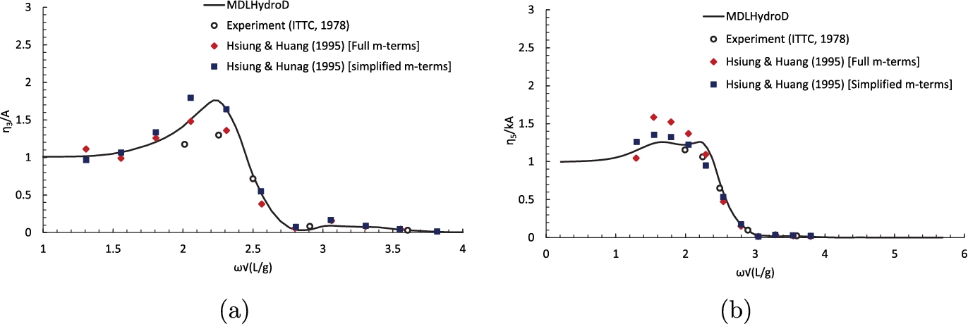
The model test results of Wigley hull III performed by Journée [22] were also compared with the developed code along with other published work by Seo et al. [43]. The heave and pitch motion comparison for the Wigley hull III is shown in Fig. 12. A full form tanker KVLCC2 is also analyzed at forward speed corresponding to $F n = 0.142$ . The panel model of the KVLCC2 is shown in Fig. 13 and the principal particulars are given in Table 3. The results were compared with experimental results of Lee et al. [30] and numerical results of Seo et al. [43] as shown in Fig. 14.

The forward speed case has been further validated against experimental result published in [8,21] and the numerical predictions of Hsiung and Huang [19] for the container ship S175. The vessel’s panel model is shown in Fig. 15 and the principal particulars are listed in Table 4.

Fig. 16.

Heave (a) and pitch (b) response of ITTC container ship S175 in head wave at $Fn = 0.25$ . (Colors are visible in the online version of the article; https://dx-doi-org.web.bisu.edu.cn/10.3233/ISP-150118.)

Fig. 17.

Heave (a) and pitch (b) response of ITTC container ship S175 in head wave at $Fn = 0.275$ . (Colors are visible in the online version of the article; https://dx-doi-org.web.bisu.edu.cn/10.3233/ISP-150118.)

Fig. 18.

Heave (a) and pitch (b) response of ITTC container ship S175 in oblique wave ( $β = 150 deg$ ) at $Fn = 0.275$ . (Colors are visible in the online version of the article; https://dx-doi-org.web.bisu.edu.cn/10.3233/ISP-150118.)

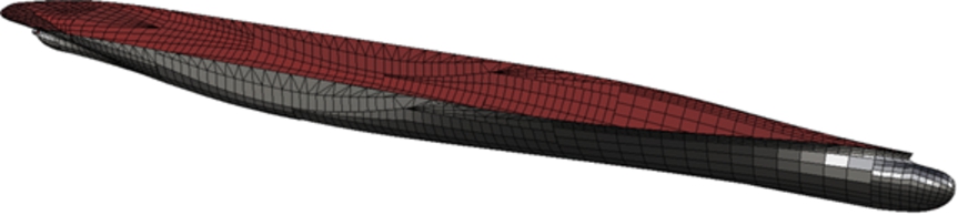
In head sea condition the heave and pitch motion amplitudes are compared for two forward speed cases with $Fn = 0.25$ and $Fn = 0.275$ shown in Figs 16 and 17, respectively. Motion of the vessel in oblique sea with wave heading $β = 150$ deg is presented in Fig. 18.

Fig. 19.

Panel model of the KRISCO Container Ship. (Colors are visible in the online version of the article; https://dx-doi-org.web.bisu.edu.cn/10.3233/ISP-150118.)

Table 5

Principal particulars of KCS

Principal particulars
Length between perpendiculars ( $Lpp$ )	230 m
Length at waterline ( $Lwl$ )	232.5 m
Breadth ( $Bwl$ )	32.2 m
Depth (D)	19 m
Draft (T)	10.8 m
Displacement (Δ)	52,030 m³
CB	0.651
CM	0.985
LCB (%), fwd+	−1.48
GM	0.6
$k_{x x} / B$	0.4
$k_{z z} / L$	0.25

Fig. 20.

Heave (a) and pitch (b) response of KCS in head sea at $Fn = 0.26$ .

Fig. 21.

Heave (a) and pitch (b) response of KCS in head sea at $Fn = 0.33$ .

Fig. 22.

Heave (a) and pitch (b) response of KCS in head sea at $Fn = 0.40$ .

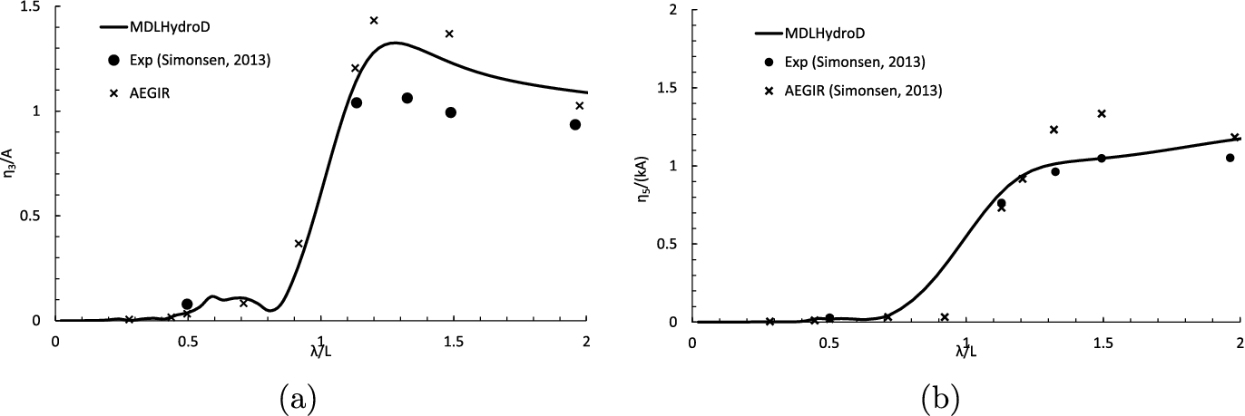
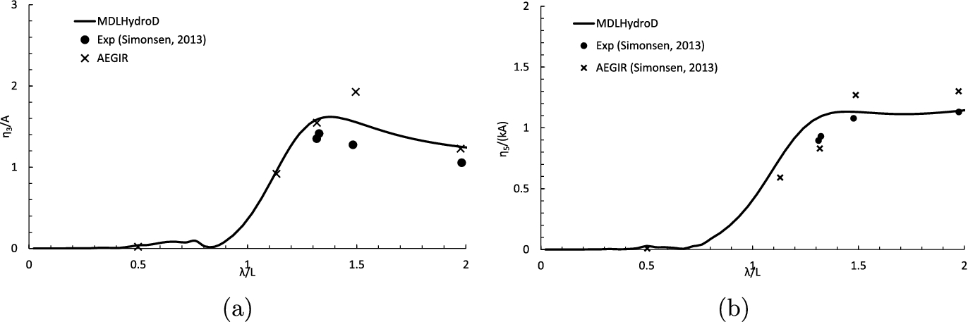
Finally, the KRISCO Container Ship (KCS) was analyzed and compared with the experiments performed by Simonsen et al. [44]. The panel model of KCS is shown in Fig. 19 and the principal particulars are given in Table 5. Three forward speed cases with $Fn = 0.26, 0.33 and 0.40$ were tested. The experimental results were also compared with a Rankine source based code named AIGER [28] along with MDLHydroD. The vertical motions for the three Froude numbers are presented in Figs 20, 21 and 22, respectively.

The comparison between the experimental and other presented numerical methods are found to agree reasonably well with the developed frequency domain program MDLHydroD. The author further extended the program for calculating second-order mean drift forces and added resistance of ships which is presented in [12,46]. An effort in developing time-domain response prediction tool using impulse response function that is based on MDLHydroD is also made. The details of this time-domain tool named SIMDYN is presented in [45,47].

5. Conclusions

A new numerical tool capable of calculating hydrodynamic force coefficients for ships with moderate forward speed in the frequency domain is developed. The effect of forward speed is included using the encounter frequency. The simplified m-terms in the radiation boundary conditions are applied. The zero speed infinite depth Green function is used in the source distribution in a quadrilateral panel discretization. Analytical expressions are used for integration of the frequency independent portion of the Green function and frequency dependent part is considered constant over a panel. The notable strengths of the developed computer program can be summarized as:

Only underwater hull surface is required for calculation, eliminating the requirement of free surface discretization. This makes the program suitable for use in hull optimization where an automatically generated panel needs to be analyzed.

A generalized coordinate system used rather than common assumption of origin at the waterline or at the center of gravity. This allows analysis of floating and submerged bodies using the same code.

The frequency independent part of the Green function has been evaluated analytically which enhance the runtime performance of the code.

Effect of forward speed is included in the hydrodynamic force calculations.

Added mass and damping coefficients can be calculated for zero and infinite frequencies with forward speed considerations. This is important for frequency to time-domain conversion using impulse response functions.

A common Geometric Data File (GDF) format is used for panel definition which makes the input files preparation for new vessels much easier and faster.

The run time of the developed code in a personal computer was found to be in order of a few seconds for a single frequency calculation of a large ship hull (2000 panels).

A number of validation studies were performed of which a selected few are presented here. The results were found to be in good agreement with experimental and other numerical results. The program has been used in further development of advanced hydrodynamic studies including non-linear time-domain response prediction and second-order force calculations.

Footnotes

Acknowledgements

The authors would like to thank Dr. F. Noblesse and Dr. K.A. McTaggart for their guidance during development of this project. This work has been funded by the Office of Naval Research (ONR) – ONR Grant N00014-13-1-0756. The authors thank Dr. Robert Brizzolara for facilitating the funding for this work.

References

[1]

Ba and

Guilbaud, A fast method of evaluation for the translating and pulsating Green’s function, Ship Technology Research (Schiffstechnik) 42(2) (1995), 68–80.

[2]

R.F.

Beck and

Liapis, Transient motions of floating bodies at zero forward speed, Journal of Ship Research 31(3) (1987), 164–176.

[3]

H.B.

Bingham, Computing the Green function for linear wave–body interaction, in: 13th International Workshop on Water Waves and Floating Bodies, 1998, pp. 5–8.

[4]

Cook,

Kill and

Hambly, Rhinoceros modeling tools for designers, Training manual level 1, Robert McNeel & Associates, Seattle, WA, USA, 2013.

[5]

Faltinsen, Sea Loads on Ships and Offshore Structures, Cambridge Univ. Press, Cambridge, UK, 1993.

[6]

O.M.

Faltinsen, Hydrodynamics of High-Speed Marine Vehicles, Cambridge Univ. Press, 2005.

[7]

Filkovic, Theory and implementation of structured 3D panel method, Master thesis, University of Zagreb, Croatia, 2008.

[8]

Fonseca and

C.G.

Soares, Experimental investigation of the nonlinear effects on the vertical motions and loads of a containership in regular waves, Journal of Ship Research 48(2) (2004), 118–147.

[9]

C.J.

Garrison, Hydrodynamic loading of large offshore structures: Three-dimensional source distribution methods, in: Numerical Methods in Offshore Engineering,

Zienkiewicz Lewis and

K.O.

Stagg, eds, John Wiley & Sons, Chichester, UK, 1978, pp. 87–139.

10.

[10]

Gerritsma and

Beukelman, Analysis of the Modified Strip Theory for the Calculation of Ship Motions and Wave Bending Moments, TNO, 1967.

11.

[11]

Guha, Development of a computer program for three dimensional frequency domain analysis of zero speed first order wave body interaction, Master thesis, Texas A&M University, College Station, TX, 2012.

12.

[12]

Guha and

Falzarano, The effect of hull emergence angle on the near field formulation of added resistance, Ocean Engineering 105(1) (2015), 10–24.

13.

[13]

Guha and

J.M.

Falzarano, Development of a computer program for three dimensional analysis of zero speed first order wave body interaction in frequency domain, in: Proceedings of the ASME 2013 32nd International Conference on Ocean, Offshore and Arctic Engineering, Nantes, France, 2013, pp. 1–9.

14.

[14]

Guha,

Somayajula and

J.M.

Falzarano, Analysis of causeway ferry dynamics for safe operation of improved navy lighterage system, in: Proceedings of the 13th International Ship Stability Workshop 2012, Brest, 2013, pp. 1–8.

15.

[15]

He and

Kashiwagi, Time-domain analysis of steady ship–wave problem using higher-order BEM, International Journal of Offshore and Polar Engineering 24(1) (2014), 1–10.

16.

[16]

He, An iterative Rankine boundary element method for wave diffraction of a ship with forward speed, Journal of Hydrodynamics, Ser. B 26(5) (2014), 818–826.

17.

[17]

J.L.

Hess and

A.M.

Smith, Calculation of non-lifting potential flow about arbitrary three-dimensional bodies, Journal of Ship Research 8(3) (1964), 22–44.

18.

[18]

J.L.

Hess and

D.C.

Wilcox, Progress in the solution of the problem of a three-dimensional body oscillating in the presence of a free surface, Technical report, MCDONNELL DOUGLAS, McDonnell Douglas Corp, Long Beach, CA, USA, 1969.

19.

[19]

Hsiung and

Huang, The frequency-domain prediction of added resistance of ships in waves using a near-field, 3-dimensional flow method, Final report, 1995.

20.

[20]

Inglis and

Price, Motions of Ships in Shallow Water, Transactions of Royal Institution of Naval Architects, 1980, pp. 269(i).

21.

[21]ITTC Seakeeping Committee, Comparison of results obtained with compute programs to predict ship motions in six-degrees-of-freedom and associated responses, in: Proceedings of the 15th ITTC, Hague, 1978, pp. 79–92.

22.

[22]

Journee, Experiments and calculations on 4 Wigley hull forms in head waves, Technical report, Delft University of Technology, Delft, The Netherlands, 1992.

23.

[23]

Kashiwagi,

Ikeda and

Sasakawa, Effects of forward speed of a ship on added resistance in waves, International Journal of Offshore and Polar Engineering 20(3) (2010), 196–203.

24.

[24]

Kashiwagi and

Wang, A new slender-ship theory valid for all oscillatory frequencies and forward speeds, in: Proceedings of the ASME 2013 32nd International Conference on Ocean, Offshore and Arctic Engineering, Nantes, France, 2013, pp. 1–8.

25.

[25]

Katz and

Plotkin, Low-Speed Aerodynamics, Vol. 13, Cambridge Univ. Press, Cambridge, UK, 2001.

26.

[26]

Kjellberg,

Contento and

C.E.

Janson, A fully nonlinear potential flow method for three-dimensional body motions, in: NAV 2012 17th International Conference on Ships and Shipping Research, Napoli, 2012, pp. 117–118.

27.

[27]

B.V.

Korvin-Kroukovsky and

W.R.

Jacobs, Pitching and heaving motions of a ship in regular waves, Transactions of the Society of Naval Architects and Marine Engineers, 1957, p. 43.

28.

[28]

D.C.

Kring, Time-domain ship motions by a 3-D Rankine panel method, PhD dissertation, Massachusetts Institute of Technology, 1994.

29.

[29]

C.H.

Lee, User manual, WAMIT, 2013.

30.

[30]

J.H.

Lee,

M.G.

Seo,

D.M.

Park,

K.K.

Yang,

K.H.

Kim and

Kim, Study on the effects of hull form on added resistance, in: Proceedings of the 12th International Symposium on Practical Design of Ships and Other Floating Structures, 2013.

31.

[31]

S.J.

Liapis, Time-domain analysis of ship motions, PhD thesis, University of Michigan, Ann Arbor, 1986.

32.

[32]

K.A.

McTaggart, Three dimensional ship hydrodynamic coefficients using the zero forward speed Green function, Technical report, Defence R&D Canada, Defence Research Development Canada, Ottawa, 2002.

33.

[33]

C.C.

Mei, Numerical methods in water-wave diffraction and radiation, Annual Review of Fluid Mechanics 10(1) (1978), 393–416.

34.

[34]

Nakos and

Sclavounos, Ship motions by a three-dimensional Rankine panel method, in: 18th Symposium of Naval Hydrodynamics, 1991.

35.

[35]

D.E.

Nakos,

Kring and

P.D.

Sclavounos, Rankine panel methods for transient free-surface flows, in: 6th International Conference on Numerical Ship Hydrodynamics, University of Iowa, Iowa City, IA, USA, National Academy Press, 1994, pp. 613–632.

36.

[36]

J.N.

Newman, The theory of ship motions, in: Advances in Applied Mechanics, Vol. 18, 1978, pp. 222–280.

37.

[37]

J.N.

Newman, Double-precision evaluation of the oscillatory source potential, Journal of Ship Research 28(3) (1984), 151–154.

38.

[38]

J.N.

Newman and

Sclavounos, The unified theory of ship motions, in: 13th Symposium on Naval Hydrodynamics, Tokyo, 1980, p. 22.

39.

[39]

Petersen, Non-linear strip theories for ship response in waves, PhD thesis, Technical, University of Denmark, 1992.

40.

[40]

Ponizy,

Noblesse,

Ba and

Guilbaud, Numerical evaluation of free-surface Green functions, Journal of Ship Research 38(3) (1994), 193–202.

41.

[41]

Qiu and

Peng, Computation of forward-speed wave–body interactions in frequency domain, International Journal of Offshore and Polar Engineering 17(2) (2007), 125–131.

42.

[42]

Salvesen,

E.O.

Tuck and

O.M.

Faltinsen, Ship motions and sea loads, Transactions of the Society of Naval Architects and Marine Engineers 78 (1970), 250–287.

43.

[43]

M.G.

Seo,

K.K.

Yang,

D.M.

Park and

Kim, Numerical analysis of added resistance on ships in short waves, Ocean Engineering 87 (2014), 97–110.

44.

[44]

C.D.

Simonsen,

J.F.

Otzen,

Joncquez and

Stern, EFD and CFD for KCS heaving and pitching in regular head waves, Journal of Marine Science and Technology 18(4) (2013), 435–459.

45.

[45]

Somayajula and

Falzarano, Large-amplitude time-domain simulation tool for marine and offshore motion prediction, Marine Systems & Ocean Technology 10(1) (2015), 1–17.

46.

[46]

Somayajula,

Guha,

Falzarano,

H.-H.

Chun and

K.H.

Jung, Added resistance and parametric roll prediction as a design criteria for energy efficient ships, Ocean Systems Engineering 4(2) (2014), 117–136.

47.

[47]

A.S.

Somayajula and

J.M.

Falzarano, Validation of Volterra series approach for modelling parametric rolling of ships, in: 34th International Conference on Ocean, Offshore and Arctic Engineering, St. John’s, Newfoundland, Canada, 2015.

48.

[48]

St. Denis and

Pierson, On the motions of ships in confused seas, in: Transactions of the Society of Naval Architects and Marine Engineers, New York, 1953, p. 81.

49.

[49]

J.G.

Telste and

Noblesse, Numerical evaluation of the Green function of water-wave radiation and diffraction, Journal of Ship Research 30(2) (1986), 69–84.

50.

[50]

Wakabayashi, Hydrodynamic study on added resistance by means of wave pattern analysis, Master thesis, Osaka University, Japan, 2012.