Statistical Methodology for Multiclass Classifications: Applications to Dementia

Abstract

Alzheimer’s disease (AD) is a common, devastating disease which carries a heavy economic burden. Accelerated efforts to identify presymptomatic stages of AD and biomarkers to classify the disease are urgent needs. Currently, no biomarkers can perfectly discriminate individuals into multiple disease categories of AD (no cognitive impairment, mild cognitive impairment, and dementia). Although many biomarkers for diagnosis and their various features are being studied, we lack advanced statistical methods which can fully utilize biomarkers to classify AD accurately, thereby facilitating evaluation of putative markers both alone and in combination. In this paper, we propose two approaches: 1) a forward addition procedure in which we adapt an additive logistic regression model to the setting for disease with ordered multiple categories. Using this approach, we select and combine multiple cross-sectional biomarkers to improve diagnostic accuracy, and 2) a method by extending the Neyman-Pearson Lemma to the ordered three disease categories to construct optimal cutoff points to distinguish multiple disease categories. We evaluate the robustness of the proposed model using a simulation study. Then we apply these two methods to data from the Religious Orders Study to examine the feasibility of combining biomarkers, and compare the diagnostic accuracy between the proposed methods and existing methods including model-based methods (ordinal logistic regression and quadratic discriminant analysis), a tree-based method CART, and the Youden index method. The two proposed methods facilitate evaluations of biomarkers for conditions with graded, rather than binary, classifications. The evaluation of the performance of different approaches provides guidance of how to choose approaches to address research questions.

Keywords

Alzheimer’s disease diagnostic accuracy generalized additive model multiclass classification optimal cutoff point volume under the surface

INTRODUCTION

Alzheimer’s disease (AD) is the most common cause of dementia in those aged 65 and above. It is one of the most persistent and devastating dementing disorders and it is the 6th most common cause of death in US according to death certificates [1]. The AD process begins with a preclinical stage during which no clinical symptoms can be detected even in very sensitive tests. As individuals approach dementia, they exhibit a progressive decline in cognitive skills and changes in behavior. Eventually individuals suffer a complete loss both of memory and of the ability to function independently [2]. The American Alzheimer’s Association projected that the number of individuals with AD in the US will grow to as many as 16 million by mid-century [2]. The biggest risk factor for AD is age and because of the aging of populations worldwide, this disease is reaching epidemic proportions with an enormous human and economic burden. For example, the estimated cost was $148 billion in 2007, was $172 billion in 2010, and will be a trillion dollars by 2050 unless preventive methods or disease-modifying treatments are identified and widely adopted [2, 3].

The criteria for clinical diagnosis of AD have been updated recently to incorporate scientific advances in the field. The new criteria include three ordered phases, which we will refer to as multiclass AD categories: the asymptomatic and preclinical phase; the symptomatic and pre-dementia phase, which is now recognized as an early stage of AD and is a transition stage from normal aging to the more serious problems caused by AD; and the dementia phase [4, 5]. Currently, the diagnosis of dementia of the AD in living patients is a clinical judgment based on neurologic and/or neuropsychological examination combined with other clinical tests. Hence, accelerated efforts to identify early and presymptomatic stages of AD, identify biomarkers to monitor disease progression, and classify individuals into different disease categories are urgent needs because of the following reasons: 1) when the clinical symptoms are detected, it is possible that the pathological disease process has been presenting for many years, 2) no pharmaceutical treatments are effective during the late stages of disease, and 3) early diagnosis may lead to the delay, prevention, or treatment of the disease and improve the quality of life for many patients.

Extensive research has been done on biomarkers of AD and there are many biomarkers (e.g., neuroradiological markers, cerebrospinal fluid (CSF) biomarkers, and peripheral biomarkers) that have been identified and various features of these biomarkers are being studied. Different biomarkers may be expressed differently in different AD stages, and different biomarkers may have different uses in diagnosing, predicting, and monitoring AD patients. Effective biomarker tests could complement existing methods to make earlier, accurate diagnosis of AD possible and identify persons at risk of advancing to clinically evident AD. However, most biomarkers are not appropriate for routine diagnostic use due to expense, side effects, requirement for specialized equipment or laboratories, and so on. For example, the CSF biomarker is invasive and the analysis may be impossible in local laboratories [6], and neuroimaging to detect AD biomarkers is expensive [7]. Currently, there are no biomarkers that can perfectly discriminate individuals into multiclass AD categories. One reason could be that we lack sophisticated statistical analysis methods which can fully utilize biomarkers to accurately classify individuals into each AD category for clinical and research purposes, and facilitate evaluation of putative markers, both alone and in combination. Statistical methods for classifying multiclass AD using multiple biomarkers will provide a better statistical framework to evaluate biomarkers as well as facilitate their use in early detection of AD and in the application of guidelines for clinical settings.

Receiver operating characteristic (ROC) curves and the area under the ROC curve (AUC) summary measure are the standard statistical tools used to evaluate the diagnostic potential of biomarkers and diagnostic tests for disease with two categories (2-class problems). While a large AUC corresponds to a biomarker for which cutoff points can be chosen to achieve high sensitivity and specificity, the AUC does not determine cutoff points. ROC measures have been extended to handle three categories (3-class problems) using volume under the surface (VUS). For example, Scurfield [8] extended the 2-class ROC to a finite number (≥3) of classes and provided a theoretic derivation of generalization of the 2-class AUC. Mossman [9] developed high-dimensional ROC concepts and estimated VUS using probabilistic ratings. Dreiseitl et al. [10] developed a non-parametric estimate of VUS and its associated variance for VUS using probabilistic ratings. Several other researchers estimated VUS for ordered disease categories. For example, Nakas and Yiannoutsos [11] developed a non-parametric estimate of VUS and its variance for disease with three ordered categories and applied the method to continuous and ordinal outcomes. Xiong et al. [12] proposed a parametric estimation of VUS and its confidence interval for disease with three ordinal diagnostic categories, assuming normal distributions of the biomarker from each diagnostic category. In addition, Li and Fine [13] used a forward selection approach for variable selection, where the estimated class probabilities from multinomial logistic regressions were used as inputs for statistical inference about hypervolume under the manifold with more than three disease categories. But the authors left several statistical issues unanswered, such as how to handle multicollinearity in covariates in the model.

Selection of cutoff points in 2-class problems is well studied [14]. For the 3-class problems, the cutoff point selection method has been described in a theoretical context in He and Frey [15]. Nakas et al. [16] and Luo and Xiong [17] studied the generalization of the Youden index to three dimensions as an index for cutoff point selection to assess the diagnostic accuracy when there were three ordinal diagnostic groups. Parametric and nonparametric methods were presented to estimate the optimal Youden index, the underlying optimal cutoff points, and the associated confidence intervals. The parametric methods in both papers assumed that biomarkers in each disease category followed normal distributions.

Aim of the research

In this paper, we will address the following question: how to effectively use existing cross-sectional biomarkers to improve diagnostic accuracy for disease with ordered three categories? We propose two methods: 1) a method to select and combine potential cross sectional biomarkers, which can significantly predict AD progression, and 2) a method to construct optimal cutoff points to distinguish multiple ordered disease categories. In addition, we compare the proposed methods with existing methods, including model-based methods (ordinal logistic regression (OLR) and quadratic discriminant analysis (QDA)), a tree-based method CART, and the Youden index method, to evaluate the diagnostic performance of different methods and to provide guidance on how to use those methods. For this step of the research, we focus on biomarkers which are cheaper, less invasive, more easily accessible for living participants, and may contain more or less information about the disease and its progression. For example, those biomarkers could be cognitive function, motor function, and blood samples.

We have organized the paper in the following manner: In the Materials and Method, we first introduce the application dataset of Religious Orders Study (ROS), and then we propose two methods 1) a forward addition procedure for variable selection and combination by adapting an additive logistic regression model and a stopping rule for adding additional covariates into the model, and 2) an approach to construct optimal cutoff points to distinguish multiple disease categories by extending Neyman-Pearson Lemma (NPL) approach to the setting for disease with multiple ordered categories. In the Simulation Section, we assess the robustness of the proposed approach. In the Results, we apply the proposed methods on the ROS dataset, and then we compare the proposed methods with several other existing approaches. Our metrics for comparison are 1) the diagnostic accuracy and the variables selected using different approaches, 2) the diagnostic accuracy between VUS and the pair-wise ROC (i.e., ROCs of biomarker 1 versus 2, 1 versus 3, 2 versus 3, 1 versus 2 & 3, and 1 & 2 versus 3) to determine whether or not VUS will provide a superior classification, and 3) the correct classification rate (CCR) using optimal cutoff points constructed using the NPL and other existing approaches. We summarize the advantages of the proposed approaches and comparison results of diagnostic accuracies between the proposed methods and other existing approaches in the Discussion Section.

MATERIALS AND METHODS

Data

The ROS [18], which is a longitudinal clinical-pathologic cohort study of aging and AD, enrolls Catholic nuns, priests, and lay brothers from more than 40 groups across the United States. Participants are without known dementia at the enrollment. The study collects various data, but we are interested in the following measures, which are collected annually: cognitive group diagnosis (no cognitive impairment (NCI), mild cognitive impairment (MCI), and AD), cognitive function measures (e.g., composite measure of episodic memory, semantic memory, and working memory), motor function measures (e.g., composite measure of manual strength, manual dexterity, and gait), disabilities and blood tests, genetic risk factors, and demographic and psychological traits. We use the last available and valid measurements from each participant for this analysis. We have total of 818 observations in the analysis dataset.

We randomly selected 20% of the data from each disease category as the test set (N = 164) and the rest used as the training set (N = 654). We fit the model using the training set, tested the classification performance of the model using the test set, and compared the classification results on both training set and test set. The variables related to cognitive function measure and motor function measure are summary scores or z scores instead of raw data. Table 1 lists the variables selected by at least one of the methods presented in this paper and the detailed information of those variables are presented in the Supplementary Material. Detailed information about the individual tests and the derivation of the composite measure has been previously reported [19 –22]. Table 2 presents mean and standard deviation (for continuous variables) and percentage (for categorical variables) for demographics and those selected variables listed in (Table 1) by three disease categories. Supplementary Table 1, a similar table of (Table 2) separated by training dataset and test dataset, is presented in the Supplementary Material.

Table 1

Variables selected by at least one method

Measure	Variable Name	Interpretation
Cognitive Function	scmmse30	Mini-Mental State Examination, 30 item standardized screening measure for delirium
	cogep cogpo cogps cogse cogwo globcog	Episodic memory Visuospatial ability Perceptual speed Semantic memory Working Memory Mean cognitive z score
Motor	rawgripavg	Grip Dynamometer
Function	rawpinchavg	Pinch Dynamometer
Disability	Katzsum	Katz measure of disability

Table 2

Demographics and variables selected by at least one method

Variable	NCI	MCI	AD
	%	%	%
Male	63.2%	71.7%	69.1%
Female	36.8%	28.3%	30.9%
Mean (SD)	Mean (SD)	Mean (SD)
Age at baseline	72.8 (6.4)	77.3 (6.7)	79.8 (6.9)
Education	18.6 (3)	17.9 (3.4)	17.7 (3.5)
Episodic memory (cogep)	0.52 (0.58)	–0.44 (0.79)	–2.38 (1.09)
Visuospatial ability (cogpo)	0.2 (0.68)	–0.58 (0.67)	–1.3 (0.88)
Perceptual speed (cogps)	–0.01 (0.86)	–0.78 (0.81)	–2.21 (0.92)
Semantic memory (cogse)	0.15 (0.61)	–0.41 (0.67)	–1.97 (1.28)
Working memory (cogwo)	0.07 (0.64)	–0.46 (0.59)	–1.41 (0.89)
Mean cognitive z-score (globcog)	0.24 (0.47)	–0.5 (0.43)	–2.02 (0.92)
Mini mental state (scmmse30)	28.3 (1.6)	26.6 (2.5)	14.2 (8.3)
Grip dynamometer (rawgripavg)	47.5 (19.5)	37.6 (16.6)	30.6 (16.9)
Pinch dynamometer (rawpinchavg)	11.1 (5.5)	9.1 (5.4)	8.2 (4.6)
Katz measure (katzsum)	0.71 (1.44)	1.27 (1.76)	3.4 (2.3)

NCI, no cognitive impairment; MCI, mild cognitive impairment; AD, Alzheimer’s disease; SD, standard deviation.

Method

In this section, we first propose two methods: 1) a forward addition procedure for variable selection and combination using cross-sectional biomarkers to improve the diagnostic accuracy in which we adapt the additive logistic regression model to the setting for disease with ordered multiple categories, and 2) a statistical approach to construct optimal cutoff points to distinguish the three ordered disease categories (NCI, MCI, and AD) by extending the NPL approach to the ordered three disease categories.

Forward addition procedure for variable selection and combination

The gold standard diagnosis of AD requires brain autopsy, which is impossible for living patients. A neuropathologist diagnoses AD if two pathognomonic signs of AD (amyloid plaques and neuritic tangles) are both found when brain tissue is examined under the microscope. In current clinical practice, the diagnosis of AD requires a uniform structured clinical evaluation which includes examining medical history, neurological examination, and cognitive testing. Based on these evaluations, a person will be classified with respect to dementia and AD according to National Institute of Neurological and Communicative Disorders and Stroke/Alzheimer’s Disease and Related Disorders Association criteria [21]. Effective biomarker tests could complement existing methods to make earlier accurate diagnosis possible and identify people at risk of advancing to clinically evident AD.

Li and Fine [13] described a forward selection approach for variable selection using multinomial logistic regression. In the following, we propose a procedure which not only selects and combines biomarkers to improve the diagnostic accuracy but also addresses the following issues (in this and the next section): 1) how to handle covariates to be added which are highly correlated with variables already entered in the model, 2) how to investigate where misclassification is occurring, and 3) how to set up a stopping rule for adding new covariates into a model.

We assume there are P biomarkers (continuous or categorical measure) denoted by Y = (Y ₁, Y ₂, … , Y_P ). Let the ordered true disease categories be denoted by D. Here NCI will be denoted by D = 1, MCI by D = 2, and AD by D = 3.

We adapt an additive ordinal logistic regression (ALR) model, which is one form of the vector generalized additive model [23, 24], to the setting of disease with ordered three categories. This model provides a flexible method to identify and characterize predictors’ nonlinear regression effect. The model has the form

$\begin{matrix} logitP (D = j | Y) = a_{j} + g_{1} (Y_{1}) \\ + g_{2} (Y_{2}) + . . . g_{p} (Y_{p}) \end{matrix}$ (1)

where the reference group is NCI (D = 1), p = 1, 2, … , P, and j = 2, 3. The function g is an estimated smoothing function of that marker to fit the data. Depending on the data, for example, the smoothing function could be a linear function, a cubic smoothing function, or some other type of parametric or nonparametric functions. The details of the methods and the smoothing functions are presented in the book and the paper by Yee et al. (VGAM) [23, 24]. Different biomarkers may have different smoothing functions and the generalized cross validation can be used to select the optimal smoothing functions. To distinguish different disease categories, we will use the sum of the combined biomarker functions selected through the model as a new diagnostic marker to classify individuals into different disease categories, estimate VUS, and construct the optimal cutoff points. This new diagnostic marker, denoted by r(Y) where r(Y) = g ₁(Y ₁)+g ₂(Y ₂)+ … +g_p (Y _p ), is the composite risk score. The disease category 3 represents the worst disease stage with the lowest biomarker measurements, r(Y), compared with the biomarker measurements from the other two categories. To fit the model (1), we need to test the proportional odds assumption. If the assumption is satisfied, we will fit a proportional odds model (i.e., the parameter estimates associated with g ₁(Y ₁), … , g_p (Y _p ) are the same for all js). If the assumption is not satisfied, we will fit either a partial proportional odds model (the parameter estimates associated with g functions are the same for some js but are different for other js) or a non-proportional odds model (each g function has its own associated parameter estimate for each j).

There are several questions we need to address when we fit the model. The first question is, which covariates can be added into the model? We usually have a large number of covariates measured from each individual which can be added into the model but often time they are correlated. If covariates are highly correlated, most likely they represent the same aspect of disease and will not add additional information to the model. Hence, we only considered adding those covariates whose multiple correlations with the covariates in the model are less than 0.8. This step is necessary especially when we encounter a huge number of covariates. We will discuss details in the Discussion.

The second question is, how to decide which biomarkers should stay in the final model? The following forward addition procedure is used to build a parsimonious model, to combine selected biomarkers, and meanwhile to maintain the best classification performance (i.e., with the largest VUS). This approach is similar to the forwarding variable selection in the paper by Li and Fine [13]. In the first step, we model one biomarker at a time to obtain r(Y) (where r(Y) = g_p (Y _p ), p = 1, 2, … P) using equation (1) and use the method in the paper by Luo and Xiong [17] to estimate the VUS in which r(Y) is used as a marker, then we pick up the biomarker which gives the largest VUS and keep this biomarker in the model. After the first step, the model (1) is $logitP (D = j | Y) = a_{j} + g_{1} (Y_{1}), j = 2, 3$ (2)

In the second step, we identify the second biomarker, which can be added in the model. We start the model with the biomarker selected from the first step (model (2)) and consider only other biomarkers, if any, whose correlation coefficient with the selected biomarker (Y ₁) in the first step is less than 0.8. We then add each of these biomarkers into the model one at a time to obtain r(Y) (where r(Y) = g ₁(Y ₁)+g_p (Y _p ), p = 1, 2, …) and estimate the VUS using r(Y) as a marker, then we pick up the second biomarker which gives the largest VUS combined with the first biomarker, and keep these 2 biomarkers in the model. After the second step, the model (1) is $\begin{matrix} logitP (D = j | Y) = a_{j} + g_{1} (Y_{1}) \\ + g_{2} (Y_{2}), j = 2, 3 \end{matrix}$

We maximize the VUS repeatedly over the remaining biomarkers.

The third question is, when should we stop adding biomarkers? The following is the proposed stopping rule. Criterion I is based on the sample size requirement. Due to the required ratio between the sample size and the number of covariates in a regression model, we stop the model-building procedure when we reach the limit of 10 observations per covariate in the group with the smallest number of participants. The second criterion is set up based on how much improvement of VUS we look for between any of two consecutive steps. Criterion II: we stop the model-building procedure when the difference between two consecutive VUS is smaller enough as determined by the point at which the VUS plateaus on a scree plot. The stopping rule we employ will be the combination of Criterion I and Criterion II.

In order to assess the diagnostic performance of the proposed method, we will compare the VUS, pair-wise AUC, and CCR between the proposed method and other existing methods including OLR, QDA, and CART approaches in the Results Section. The CCR is defined as the total number of correct classifications from all disease categories divided by the total number of individuals in the dataset. To estimate CCR, we need cutoff points to determine classification. Please refer to the next section to obtain the cutoff points for different approaches.

Optimal cutoff points

After the identified biomarkers are shown to better discriminate participants into each of the AD categories, the next step will be to determine cutoff points upon which a diagnosis can be made. Selecting cutoff points for diagnosis will be crucial in order to translate findings into medical practice and provide good interpretation of the data to support clinical diagnosis. Both parametric and nonparametric methods of selecting cutoff points for 3-class problems using the Youden index have been proposed [16, 17]. However, the method in the paper by Nakas et al. [16] is computationally intensive since many random permutations must be generated. The cutoff points constructed using the method in the paper by Luo and Xiong [17] is specifically derived for three group diagnostic tests for some parametric distributions.

For a 3-category diagnostic test, we have three true classification rates where we use T to represent the test result. Those three true classification rates are P (T = 1|D = 1), P (T = 2|D = 2), and P (T = 3|D = 3), and we have six false classification fractions, which are P (T = 2, |D = 1), P (T = 3|D = 1), P (T = 1|D = 2), P (T = 3|D = 2), P (T = 1|D = 3), and P (T = 2|D = 3). In the following, we propose to construct the optimal cutoff points using the NPL approach, which has been used to construct cutoff points for 2-class disease problems [25]. We extend the NPL approach to 3-class disease problems. The detailed derivations are given in the Supplementary Material. The composite risk score r(Y) generated using equation is used as a new diagnostic biomarker. If this composite risk score r(Y) of having disease given the observed biomarkers Y is $\begin{matrix} r (Y) < \frac{P (D = 3)}{c_{0} (f_{12, 3}) P (D \neq 3) + P (D = 3)} \\ = c^{*} (f_{12, 3}) \end{matrix}$

then the test result indicates that the disease category is 3. Since the false classification rate given the true disease categories 1 & 2, denoted by f ₀₃, is defined as

$f_{03} = P (r (Y) < c^{*} (f_{12, 3}) | (D = 1 \cup D = 2))$

we can choose c*(f _12,3), the optimal cutoff point for distinguishing disease category 1 & 2 versus 3, as the f ₀₃ quantile of the composite risk score r(Y) in the population with disease categories D = 1 and D = 2, where f ₀₃ is pre-specified. All other notations are defined in the Supplementary Material.

Similarly, if the composite risk score of having disease given the observed biomarkers Y is $\begin{matrix} r (Y) > \frac{P (D = 1)}{c_{0} (f_{23, 1}) P (D \neq 1) + P (D = 1)} \\ = c^{*} (f_23, 1) \end{matrix}$

then the test result indicates that the disease category is 1. Since the false classification rate given the true disease categories 2 & 3, denoted by f ₀₁, is

$f_{01} = P (r (Y) > c^{*} (f_23, 1) | (D = 2 \cup D = 3))$

we can choose c*(f _23,1), the optimal cutoff point for distinguishing disease category 1 versus 2 & 3, as the 1– f ₀₁ quantile of the composite risk score r(Y) in the population with disease categories D = 2 and D = 3, where f ₀₁ is pre-specified.

For the QDA approach, the cutoff point, denoted by C, to distinguish between disease category j and j + 1 is $C_{j (j + 1)} = \frac{N_{j} Z_{j + 1} + N_{j + 1} Z_{j}}{N_{j} + N_{j + 1}} for j = 1, 2$

where N_j is the total number of observations in the disease category j, N_j ₊ ₁ is the total number of observations in the disease category j + 1, Z_j is the centroid of the composite risk score in the disease category j, and Z_j ₊ ₁ is the centroid of the composite risk score in the disease category j + 1.

For the OLR approach, given the sample size and similar number of participants in each disease category, the cutoff point to distinguish between disease category 2 and 3 was selected as the 33 percentile of the composite risk score; and the cutoff point to distinguish between disease category 1 and 2 was selected as the 66 percentile of the composite risk score.

Simulation

To assess the robustness of the proposed ALR approach, we did the simulation studies. We simulated three biomarkers and the disease category for each observation. The following are assumptions of the location parameter (μ) and scale parameter (σ) for each biomarker. Some of the assumptions are based on the ROS data. For biomarker 1, μ _NCI = 0.2, σ _NCI = 0.5, μ _MCI = –0.5, σ _MCI = 0.5, μ _AD = –2, σ _AD = 0.5. For biomarker 2, μ _NCI = 11, σ _NCI = 5, μ _MCI = 9, σ _MCI = 5, μ _AD = 6, σ _AD = 4. For biomarker 3, which is a categorical variable, score_NCI ∈(0, 1, 2), score_MCI ∈(2, 3, 4), score_AD ∈(4, 5, 6). We consider the following scenarios:

Biomarker 1 and 2 in each disease category follow two distributions: bivariate normal distribution (skewness parameter γ= 0) and skewed bivariate normal distribution (with the skewness parameter γ of –0.1, –0.25, and –0.65).

The correlation coefficients (ρ) between biomarker 1 and 2 are 0, 0.1, 0.4, and 0.7.

The sample size for each disease category ranges from 20 to 300.

The prevalence of each disease category ranges from 10% to 56%.

We simulated the datasets 500 times for each scenario, and then follow the procedure described in the Method Section to fit model (1) and select biomarkers to achieve the best classification. The bias is defined as the difference of the estimated VUS between each scenario and the scenario without correlation (ρ= 0) and skewness (γ= 0). Results in (Table 3) demonstrate the following: 1) For fixed ρ and γ, when the sample size increases, the standard deviation (SD) of the estimated VUS decreases, but the bias are similar. For example, the bias of the estimated VUS between Line 4 and 1, between Line 10 and 7, between Line 16 and 13, between Line 22 and 19, between Line 28 and 25, and between Line 34 and 31. 2) For fixed γ and the sample size, when the correlation between biomarkers increases, the bias of the estimated VUS increases but the SDs are similar. For example, the bias of VUS between Line 18 and 13 is larger than that between Line 16 and 13, but the SD in Line 18 is similar to the SD in Line 16. 3) For fixed ρ and the sample size, when the skewness γ increases, both the bias and the SD are similar. For example, the bias of the estimated VUS between Line 15 and 11 is similar to the bias between Line 16 and 11 and the SD in Line 15 is similar to it in Line 16. 4) When both ρ and γ increases for fixed sample size, the bias of VUS increases but the SD are similar. 5) For different disease prevalence, the impact on the estimates of SD and the bias is minimal. Unless we have extreme datasets (e.g., very small sample size, or very skewed data, or larger correlation between observations), the results from the proposed method is robust.

Table 3

Simulation results

Line	N_NCI	N_MCI	N_AD	ρ	γ	VUS	SD
1	20	20	20	0	0	0.816	0.068
2				0.1	–0.1	0.812	0.073
3				0.4	–0.25	0.776	0.073
4				0.4	–0.65	0.778	0.076
5				0.7	–0.25	0.748	0.082
6				0.7	–0.65	0.752	0.079
7	70	20	10	0	0	0.808	0.068
8				0.1	–0.1	0.804	0.064
9				0.4	–0.25	0.766	0.067
10				0.4	–0.65	0.768	0.071
11				0.7	–0.25	0.738	0.073
12				0.7	–0.65	0.737	0.072
13	50	50	50	0	0	0.791	0.042
14				0.1	–0.1	0.779	0.043
15				0.4	–0.25	0.750	0.046
16				0.4	–0.65	0.749	0.046
17				0.7	–0.25	0.730	0.049
18				0.7	–0.65	0.725	0.045
19	50	100	200	0	0	0.783	0.034
20				0.1	–0.1	0.772	0.036
21				0.4	–0.25	0.749	0.035
22				0.4	–0.65	0.741	0.036
23				0.7	–0.25	0.719	0.037
24				0.7	–0.65	0.715	0.039
25	150	150	150	0	0	0.781	0.023
26				0.1	–0.1	0.771	0.024
27				0.4	–0.25	0.743	0.024
28				0.4	–0.65	0.743	0.024
29				0.7	–0.25	0.715	0.026
30				0.7	–0.65	0.712	0.025
31	200	100	300	0	0	0.781	0.023
32				0.1	–0.1	0.772	0.024
33				0.4	–0.25	0.744	0.024
34				0.4	–0.65	0.741	0.025
35				0.7	–0.25	0.716	0.026
36				0.7	–0.65	0.712	0.026

NCI, no cognitive impairment; MCI, mild cognitive impairment; AD, Alzheimer’s disease; VUS, volume under the surface; SD, standard deviation; ρ, correlation coefficient; γ, skewness; N, sample size.

RESULTS

In this section, we apply the proposed methods to data from the ROS and compare the selected variables and VUS among the following approaches: 1) the proposed forward addition procedure with the ALR and a stopping rule approach, 2) stepwise OLR, 3) stepwise QDA, and 4) CART. We then compare the CCRs using the cutoff points constructed by the NPL approach, the OLR approach, the QDA approach, and the CART approach. In addition, we compare the CCR and misclassification rate for each disease category using cutoff points constructed from the proposed NPL approach with those constructed using the Youden index method of Luo and Xiong [17].

Classification accuracy and variable selection

In this section, we compare the diagnostic accuracy measured by VUS, and the biomarkers selected using the proposed method with several existing methods.

We used an R package VGAM to fit the ALR model. Using the forward addition procedure with the ALR model and a stopping rule, the model selected two variables (globcog (mean cognitive z-score) and rawpinchavg (pinch dynamometer)). The smooth function for globcog is a cubic spline with degree freedom of 4 and the smooth function for rawpinchavg is a cubic spline with degree freedom of 1. From the scree plot (Fig. 1), we can see that the line of the scree plot stops increasing rapidly and levels out when we have three covariates in the model versus two covariates and the VUS plateaus on the scree plot is at the point when the model has two covariates. Hence, we only selected two covariates in the model for this example.

Fig.1

Scree plot.

The several existing methods are: 1) stepwise OLR approach where SAS proc logistic was used with the default p-values of 0.05 as the variable selection criterion: a linear combination of the biomarkers selected through the model is used as the composite risk score to estimate VUS and cutoff points, 2) stepwise QDA approach where SAS proc stepdisc was used with the default p-value of 0.15 as the variable selection criterion: the sum of combined quadratic functions of those biomarkers selected through the model is used as the composite risk score to estimate VUS and cutoff points, and 3) CART approach where the R package rpart was used. Using CART, we cannot estimate VUS since each individual’s predicted probability is the probability of the category that individual is assigned to, i.e., all individuals assigned to the same disease category share the same predicted probability at each partition step.

Table 4 presents the comparison of VUS and variables selected from different approaches. Among those approaches, the proposed forward addition procedure using the ALR model with a stopping rule provides the highest VUS for both training set and test set. It is very interesting to note that the biomarkers selected using the OLR approach and the CART approach include variables from the cognitive function only, while the biomarkers selected using the proposed ALR approach and the QDA approach include variables from both the cognitive function and the motor function. However, the ALR approach provides a much more parsimonious model with only two biomarkers selected compared with the QDA approach in which seven biomarkers were selected with four variables from the cognitive function and two variables from the motor function. In addition, the VUS obtained from the ALR approach is much larger than the VUS obtained from the stepwise QDA approach. The VUS from the test set with only two selected biomarkers is 0.75, which is considered as a satisfactory classification result. This result indicates that using the composite risk score constructed from the proposed model with the limited number of covariates can provide a reasonable classification.

Table 4

VUSs and biomarkers selected from different approaches

Approach	VUS		Selected Variables
Approach	Training Set	Test Set	Selected Variables
Forward Addition with Additive Logistic Regression Procedure (ALR)	0.87	0.75	mean cognitive z-score (globcog) pinch dynamometer (rawpinchavg)
Ordinal Logistic Regression (OLR)	0.75	0.70	episodic memory (cogep)
Quadratic Discriminant Analysis (QDA)	0.63	0.65	episodic memory (cogep) semantic memory (cogse)
			pinch dynamometer (rawpinchavg) mean cognitive z-score (globcog) mini mental state (scmmse30)
			katz measure (katzsum)
			grip dynamometer (rawgripavg)
Classification and Regression Tree (CART)	—	—	episodic memory (cogep) visuospatial ability (cogpo) mean cognitive z-score (globcog)

Pair-wise AUC versus VUS

The VUS is a summary measure of the global classification accuracy, and the pair-wise AUC is a summary measure of diagnostic test between any of the two disease categories. The question we will address in this section is whether the VUS is always superior to the pair-wise AUC. In the following, we compare the estimated VUS, pair-wise AUC, and CCR for the training set and test set where the composite risk score is estimated using the forward addition procedure using the ALR approach with the stopping rule. The cutoff points were constructed using the proposed NPL approach.

Table 5 presents the results. The pair-wise AUC and CCR for disease category NCI versus AD, MCI versus AD, NCI versus non-NCI, and non-AD versus AD are higher than the VUS and CCR for 3-class problems, which are the overall classification measures using all three categories together, for both training and test sets. The pair-wise AUC and CCR for distinguishing disease category NCI versus MCI are similar to the VUS and CCR using all three categories together.

Table 5

Comparison of pair-wise AUC, VUS, and CCR estimated using composite risk score constructed by ALR model with stopping rule for both training and test datasets

Comparison	VUS/AUC		CCR
Comparison	Training Set	Test Set	Training Set	Test Set
3-class Comparison	0.87	0.75	0.80	0.78
Pair-wise Comparison
NCI versus MCI	0.89	0.83	0.82	0.78
MCI versus AD	0.96	0.90	0.89	0.82
NCI versus AD	0.99	0.99	0.97	0.96
NCI versus non-NCI	0.92	0.91	0.86	0.86
non-AD versus AD	0.98	0.97	0.93	0.91

NCI, no cognitive impairment; MCI, mild cognitive impairment; AD, Alzheimer’s disease; VUS, volume under the surface; AUC, area under the curve; CCR, correct classification rate.

As stated in the paper by Nakas and Yiannoutsos [11], VUS is a global classification ability which shows the average chance that the biomarkers obtained from any three randomly selected individuals from disease category NCI, MCI, and AD will have the expected ordering. Therefore, the VUS is a necessary summary measure to demonstrate how accurately we could identify the trend in the biomarker measurements which is scientifically important when we simultaneously classify disease with ordered multiple categories. However, checking the pair-wise AUC and CCR provides additional information about the distinction between each pair of disease categories considered separately which allows us to identify where the misclassification occurs. For this example, disease category NCI and MCI cannot be separated very well compared with any other two disease categories although the pair-wise AUC for the test set is 0.83, which is considered to be a reasonable classification. Therefore, using VUS, which provides the overall diagnostic accuracy, and pair-wise AUC, which identifies misclassifications, together will provide more classification information than using either VUS or pair-wise AUC alone.

Classification accuracy using different cutoff points

Since the composite risk score constructed using the proposed approach can provide satisfactory classification for disease with three ordered categories, we now turn our attention to compare the performance of cutoff points by comparing the CCR and the misclassification rate using cutoff points constructed from the NPL approach (the pre-specified false classification rate f ₀₁ and f ₀₃ are 0.05) and other approaches (the approaches to select cutoff points using the OLR and QDA approaches were presented in the Optimal Cutoff Points Section) for both training set and test set in this section.

Table 6 presents the estimates and the corresponding 95% confidence intervals obtained through the bootstrap method. Overall, the CCRs using the cutoff points constructed from the NPL approach and the CART approach are better compared with the CCRs using the cutoff points constructed from the model-based approaches of OLR and QDA for both training and test sets. The reason is that the latter two methods do not employ an optimal procedure in the selection of cutoff points. In addition, the majority of the true classification rates (e.g., P (T = NCI|D = NCI)) from the NPL and the CART approaches are better than those from the OLR and QDA approaches for both training and test sets. However, the results show that none of the approaches can identify participants with MCI very well. The proposed ALR, the OLR, and the QDA approaches are all global prediction modeling approaches in which a single prediction formula is used for the entire dataset for each disease category and there is a single cutoff point based on the composite risk score— which is the sum of the combined functions of those biomarkers selected from each prediction model— to distinguish any two disease categories. In contrast, the CART approach is a recursive partition classification approach which provides a cutoff point for each biomarker selected in the model instead of using a global formula. Using the CART approach, the graph of classification and regression tree (Supplementary Figure 1) is a three-branch tree. Most of participants in disease category 1 (NCI) and all participants in disease category 3 (AD) can be clearly classified using the global composite cognitive score (globcog) at the first step of the partition. If the globcog is lower than –0.9388, then participants will be classified as AD. If the globcog is higher than –0.1232, then participants will be classified as NCI. However, for the participants whose globcogs are between –0.9388 and –0.1232, we need the episodic measure (cogep) and the visuospatial ability (cogpo) to further assist classification. Participants will be classified as MCI if the cogep is smaller than –0.4423 or the cogpo is smaller than –0.771; otherwise participants will be classified as NCI. The CART method provides a slightly higher CCR and P(T = NCI|D = NCI) for the test set compared with the CCR using the NPL approach based on the ROS dataset. Although the classification decision from the CART approach or the other three approaches are all based on the combination of the biomarkers, the decision from the CART approach is based on the combined classification from each selected biomarker at each partition step. In contrast, the decision from any of the other three model-based approaches is based on a single composite score, which is the sum of the combined functions of those selected biomarkers.

Table 6

Classification results using cutoff points from different approaches for both training and test datasets

Comparison	Training Set
Comparison	NPL	OLR	QDA	CART
CCR	0.874 (0.871,0.880)	0.612 (0.609,0.614)	0.662 (0.659,0.664)	0.838 (0.836,0.840)
P(T = NCI\|D = NCI)	0.875 (0.872,0.880)	0.572 (0.566,0.614)	0.756 (0.751,0.761)	0.949 (0.947,0.952)
P(T = MCI\|D = MCI)	0.610 (0.600,0.620)	0.433 (0.425,0.440)	0.447 (0.436,0.457)	0.602 (0.590,0.613)
P(T = AD\|D = AD)	0.945 (0.939,0.952)	0.928 (0.921, 0.935)	0.647 (0.634,0.660)	0.878 (0.869,0.886)
	Test Set
	NPL	OLR	QDA	CART
CCR	0.720 (0.710,0.730)	0.569 (0.561,0.576)	0.743 (0.733,0.752)	0.760 (0.751,0.769)
P(T = NCI\|D = NCI)	0.700 (0.680,0.730)	0.495 (0.447,0.519)	0.801 (0.781,0.822)	0.900 (0.885,0.914)
P(T = MCI\|D = MCI)	0.440 (0.392,0.492)	0.213 (0.175,0.250)	0.623 (0.586,0.660)	0.450 (0.404,0.502)
P(T = AD\|D = AD)	0.950 (0.940,0.970)	0.954 (0.935,0.973)	0.745 (0.707,0.783)	0.784 (0.750,0.818)

NCI, no cognitive impairment; MCI, mild cognitive impairment; AD, Alzheimer’s disease; NPL, Neyman-Pearson lemma; OLR, ordinal logistic regression; QDA, quadratic discriminant analysis; CART, classification and regression tree; CCR, correct classification rate; T, test results; D, disease status.

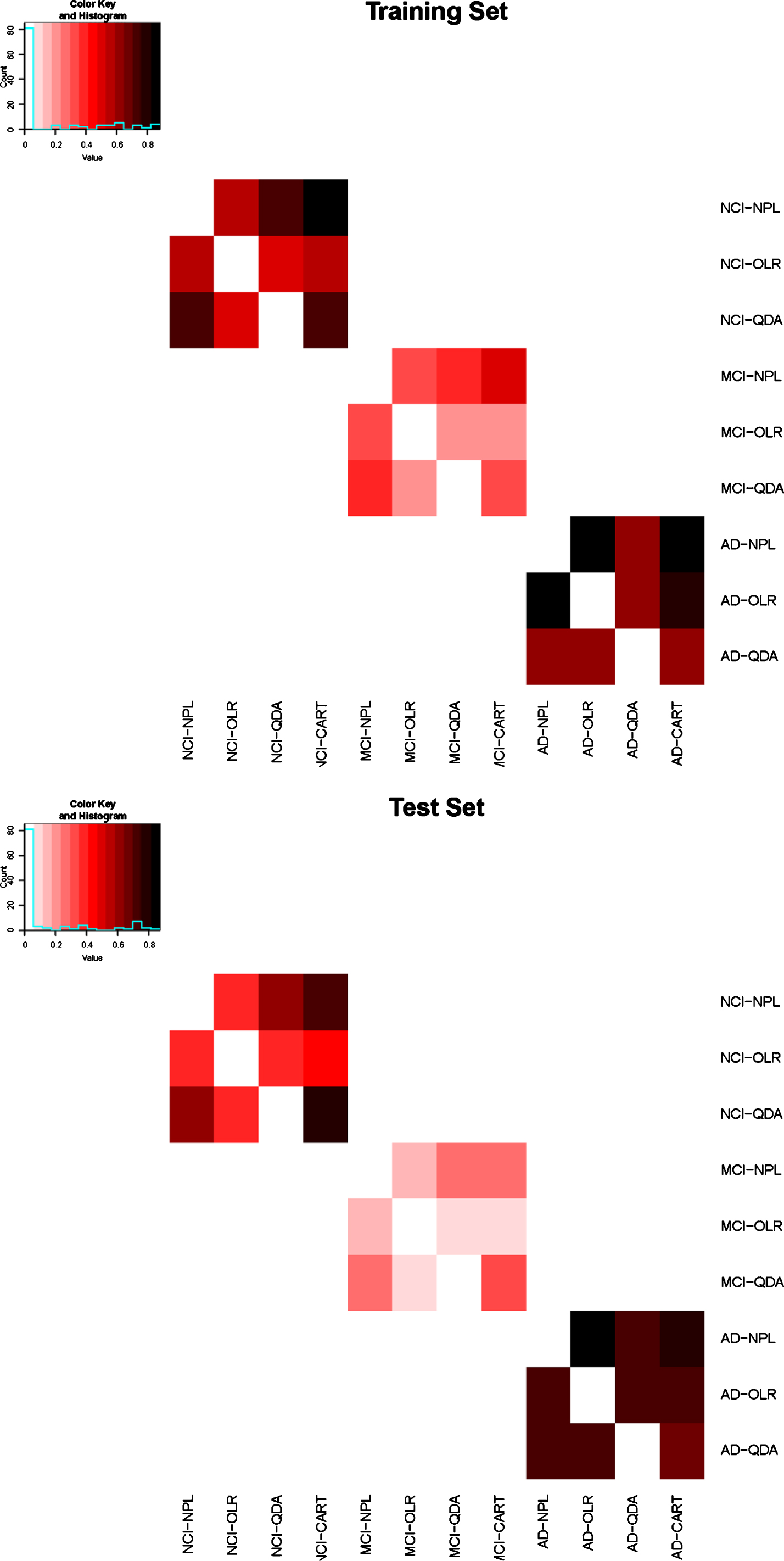
Besides evaluating the diagnostic accuracy between different approaches, we also evaluate whether the same patient can be classified into the same disease category by different approaches. The percentage of agreements, which is defined as the percentage of patients whose estimated disease category are consistent with their true disease categories and also consistent between different approaches, were calculated. The heatmap (Fig. 2) presents the percentage of agreement among different approaches for each disease category for both training and test sets. The figure shows that the NPL approach and CART approach agree well with majority of the approaches. However, the agreement between the OLR approach and the QDA approach is much lower and none of the approaches agree very well for disease category MCI.

Fig.2

Heat map.

Lastly, (Table 7) presents the comparison of the CCR, the overall misclassification rate (e.g., P(T = MCI or AD|D = NCI)), and the false classification fraction using the optimal cutoff points constructed from the NPL approach and the Youden index approach in the paper by Luo and Xiong [17]. These two approaches have very similar CCRs with the CCR using the NPL approach slightly higher than the CCR using the Youden index approach for both training and test sets. For disease category NCI and AD, the proposed NPL approach shows smaller overall misclassification rates and the false classification fractions for both training set and test set. The Youden index approach has a much larger overall misclassification rate when the true disease category is AD comparing with that using the NPL approach (The overall misclassification rate using Youden index approach is 2.6 times of that using the NPL approach in the training set and 4.25 times in the test set). For disease category MCI, the overall misclassification rate and the false classification fraction are similar between the two approaches for the training set, but the misclassification rate for the test set using the NPL approach is larger than that using the Youden index approach (The overall misclassification rate using the NPL approach is 1.7 times of that using the Youden index approach). Overall, the NPL approach performs better than the Youden index approach using the ROS data.

Table 7

CCRs and misclassification rates using optimal cutoff points constructed from NPL and Youden Index approaches for both training and test datasets

Comparison	Training Set
	NPL	Youden
	Approach	Index
CCR	0.82	0.81
P(T = MCI or AD\|D = NCI)	0.12	0.14
P(T = MCI\|D = NCI)	0.11	0.13
P(T = AD\|D = NCI)	0.01	0.01
P(T = NCI or AD\|D = MCI)	0.38	0.31
P(T = NCI\|D = MCI)	0.27	0.25
P(T = AD\|D = MCI)	0.11	0.06
P(T = NCI or MCI\|D = AD)	0.05	0.13
P(T = NCI\|D = AD)	0.00	0.00
P(T = MCI\|D = AD)	0.05	0.13
	Test Set
	NPL	Youden
	Approach	Index
CCR	0.74	0.73
P(T = MCI or AD\|D = NCI)	0.22	0.30
P(T = MCI\|D = NCI)	0.22	0.30
P(T = AD\|D = NCI)	0.00	0.00
P(T = NCI or AD\|D = MCI)	0.60	0.35
P(T = NCI\|D = MCI)	0.35	0.25
P(T = AD\|D = MCI)	0.25	0.10
P(T = NCI or MCI\|D = AD)	0.04	0.17
P(T = NCI\|D = AD)	0.00	0.00
P(T = MCI\|D = AD)	0.04	0.17

NPL, Neyman-Pearson lemma; NCI, no cognitive impairment; MCI, mild cognitive impairment; AD, Alzheimer’s disease; CCR, correct classification rate; T, test results; D, disease status.

DISCUSSION

In this paper, we proposed a forward addition procedure using the additive ordinal logistic regression model and a stopping rule to select and combine multiple cross-sectional biomarkers to improve diagnostic accuracy for disease with ordered multiple categories. Meanwhile, we addressed several statistical issues related to classification and model fitting. In addition, we developed an approach to construct the optimal cutoff points to distinguish multiple disease categories using the NPL approach. By comparing the proposed approaches with several existing approaches (stepwise OLR, stepwise QDA, CART, and Youden index approaches) on the ROS data, the analysis results show that both proposed approaches (forward addition procedure and optimal cutoff points constructed using NPL) provide much better diagnostic accuracies comparing with those existing model-based approaches and the Youden index approach. In addition, assessing VUS and pair-wise AUC, we can easily identify where the misclassification is occurring.

Because there is no single test that can determine the disease category for individuals with cognitive impairments, using the forward addition procedure we address an important practical question which is how to determinate a parsimonious set of cross sectional biomarkers which can optimally classify disease, like AD, with ordered multiple categories. The proposed methods provide very important tools to improve the diagnostic accuracy. The methods are especially important to distinguish participants with NCI versus MCI since: 1) MCI is a transitional stage of AD which indicates more serious disease development in the future, 2) MCI has important implications for initiating treatment and monitoring the progression of disease, and 3) early diagnosis of MCI provides a better chance to slow the progression of memory loss and improve the quality of life for many participants.

We proposed to use the forward addition procedure for variable selection and combination. For a disease like AD, we usually have a large pool of biomarkers to select from when we fit the model. We have about 40 biomarkers available for analysis, in which we know all those biomarkers are potential risk factors related to AD. In addition, we can easily extend the analysis to include other biomarkers, whose relation to the disease we may not know clearly. With such large pool of potential biomarkers, the forward variable selection procedure is a natural choice. The final choice of the variables in the model is based on the classification performance, i.e., we only choose the biomarkers which can provide accurate classification (i.e., the largest VUS). The analysis results of applying the proposed approach on ROS dataset shows that the proposed forward addition procedure not only addresses several important statistical issues regarding the variable selection and combination, but also provides a general procedure regarding how to effectively select and combine multiple biomarkers to improve the diagnostic accuracy for classifying disease with ordered multiple categories. In addition, the advantages of using the proposed NPL approach to construct optimal cutoff points are the following: 1) it can accommodate any number of biomarkers (continuous or categorical) using equation (1), 2) it can be easily extended to disease with any number of disease categories, 3) it can be easily computed, and 4) it can accommodate any parametric assumptions. The two proposed approaches provide general and better techniques to facilitate evaluations of existing multiple biomarkers for disease with multiple ordered categories. Through the analysis, we also learn that VUS is a necessary diagnostic accuracy summary for disease with multiple categories, but it may not be superior to a pair-wise AUC. The combination of the two summary measures may provide more information about the overall diagnostic accuracy and misclassification.

In the proposed forward addition procedure, we used an additive logistic regression model, which could be changed to other models depending on the nature of the data. In the Method section, we briefly discussed that we only considered adding those biomarkers whose correlations with the biomarkers in the model are less than 0.8. Given the sample size in this analysis, we can fit at most 20 biomarkers in the model. However, we have at least 40 biomarkers available and estimating VUS is time consuming. Hence, using the forward addition procedure, we may efficiently eliminate highly correlated biomarkers adding into the model. This efficient approach to eliminate highly correlated biomarkers is to screen the collinearity since highly correlated biomarkers may not represent different aspects of the disease and may not add additional information about disease in the model. Although collinearity does not reduce the predictive power or reliability of the model, the individual coefficients may be difficult to interpret when predictors are redundant. The reason we chose the correlation coefficient of 0.8 is the following: the variance inflation factor for the pth predictor (VIF_p) is defined as $\frac{1}{1 - R_{p}^{2}}$ (where R _p is the correlation of Y _p with the other p –1 Y ’s which were already added in the model), which measures how much the variance of an estimated regression coefficient is increased because of collinearity. In general, a value of VIF of 2.5 or above indicates a collinearity problem which is equivalent to a correlation coefficient 0.8 or above (R² is approximately equal to 0.6 or above).

In the proposed model, we used the disease category (NCI, MCI, and AD) as the outcome variable in the regression model. However, our proposed approach has a broader applicability. For example, the proposed method can be used to identify biomarkers that reflected underlying disease pathology in which the pathology categories will be the outcome variable in the regression model.

In current clinical practice, the diagnosis of AD is performed through clinical evaluation. The initial diagnosis criteria for AD was established by National Institute of Neurological and Communicative Disorders and Stroke/Alzheimer’s Disease and Related Disorders Association in 1984. Research [26] shows that the criteria defined in 1984 is reliable (with the sensitivity of 81% and specificity of 70% [27]). Since our knowledge of the clinical manifestations and biology of AD has increased vastly, these criteria were updated in 2011 which incorporated more modern innovations in clinical, imaging, and laboratory assessment [27]. These new criteria were implemented a few years ago and no research presented its sensitivity and specificity yet, but we believe the revised criteria should outperform the criteria established in 1984.

In the proposed model, we did not make the proportional odds assumption. If the proportional odds assumption is violated, we could fit either a partial proportional or a non-proportional odds model. We also could add interaction terms in the model to make the proportional odds assumption valid. In the simulation studies, we fit all models assuming the proportional odds assumption valid. However, this assumption is not always satisfied for all simulated data especially those datasets with larger skewness. Results in (Table 3) reflected the impact of the violation of the proportional odds assumption. It might be a better idea to check the proportional odds assumption before we perform the analysis.

Several results using the CART approach are better than those using the proposed approach based on the ROS dataset. One particular strength of the CART approach is its ability to identify interactions which is not considered in the proposed method. We could add interaction terms in the proposed model. However, our main interest focuses on identifying a few biomarkers (a parsimonious model) representing different aspects of the disease and estimating their main effects contributing to the classification of AD.

In this paper, we also presented how to apply existing methods to identify and combine biomarkers to classify disease with ordered multiple categories. The comparisons of the diagnostic accuracies among different approaches not only provided a summary of the overall performance of those existing methods, but also provided a pool of techniques that researchers may choose from to address their research questions.

DISCLOSURE STATEMENT

Authors’ disclosures available online (https://www.j-alz.com/manuscript-disclosures/18-0580r2).

Footnotes

The supplementary material is available in the electronic version of this article: .

References

Alzheimer’s Association (2016) Alzheimer’s disease facts and figures. Alzheimers Dement 12, 459–509.

Ward

(2007) Biomarkers for Alzheimer’s disease. Expert Rev Mol Diagn 7, 635–646.

Bateman

, Xiong

, Benzinger

TLS

, Fagan

, Goate

, Fox

, Marcus

, Cirns

, XieX Balzey, TM , Holtzman

, Santacruz

, Buckles

, Oliver

, Moulder

, Aisen

, Ghetti

, Klunk

, McDade

, Martins

, Masters

, Mayeux

, Ringman

, Rossor

, Scofield

, Sperling

, Salloway

, Morris

(2013) Clinical and biomarker changes in dominantly inherited Alzheimer’s disease. N Engl J Med 367, 795–804.

McKhann

, Knopman

, Chertkow

, Hyman

, Jack

Jr , Kawas

, Klunk

, Koroshetz

, Manly

, Mayeux

, Mohs

, Morris

, Rossor

, Scheltens

, Carillo

, Thies

, Weintraub

, Phelps

(2002) The diagnosis of dementia due to Alzheimer’s disease: Recommendations from the national institute on aging and the Alzheimer’s association workgroup. Alzheimers Dement 7, 263–269.

Jack

Jr , Albert

, Knopman

, McKhann

, Sperling

, Carrillo

, Thies

, Phelps

(2011) Introduction to the recommendations from the national institute of aging and the Alzheimer’s Association workgroup on diagnostic guidelines for Alzheimer’s disease. Alzheimers Dement 7, 257–262.

Chintamaneni

, Bhaskar

(2012) Biomarkers in Alzheimer’s disease: A review. ISRN Pharmacol 2012, 1–6.

Moreno

, Osta

, Calvo

(2015) New perspectives in the search for reliable biomarkers in Alzheimer disease. Eur J Psychiatry 29, 51–65.

Scurfield

(1996) Multiple-event forced-choice tasks in the theory of signal detectability. J Math Psychol 40, 253–269.

Mossman

(1999) Three-way ROCs. Med Decis Making 19, 78–89.

10.

Dreiseitl

, Ohno-Machado

, Binder

(1998) Comparing three-class diagnostic tests by three-way ROC analysis. Med Decis Making 20, 323–331.

11.

Nakas

, Yiannoutsos

(2004) Ordered multiple-class ROC analysis with continuous measurement. Stat Med 23, 3437–3449.

12.

Xiong

, van Belle

, Miller

, Morris

(1998) Measuring and estimating diagnostic accuracy when there are three ordinal diagnostic groups. Biostatistic 26, 1251–1273.

13.

, Fine

(2006) ROC analysis with multiple classes and multiple tests: Methodology and its application in microarray studies. Stat Med 9, 566–576.

14.

Pepe

(2003) The Statistical Evaluation of Medical Tests for Classification and Prediction. Oxford University Press.

15.

, Frey

(2006) Three-class roc analysis-the equal error utility assumption and the optimality of three-class roc surface using the ideal observers. IEEE Trans Med Imaging 25, 979–986.

16.

Nakas

, Alonzo

, Yiannoutsos

(2009) Accuracy and cut-off point selection in three-class classification problems using a generalization of the Youden index. Stat Med 29, 2946–2955.

17.

Luo

, Xiong

(2013) Youden index and associated cutpoints for three ordinal diagnostic groups. Commun Stat SimulComput 42, 1213–1234.

18.

Bennett

, Schneider

, Arvanitakis

, Wilson

(2012) Overview and finding from the Religious Orders Study. Curr Alzheimer Res 9, 628–645.

19.

Wilson

, Beckett

, Barnes

, Schneider

, Bach

, Evans

, Bennett

(2002) Individual differences in rates of change in cognitive abilities of older persons. Psychol Aging 17, 179–193.

20.

Wilson

, Barnes

, Bennett

(2003) Assessment of lifetime participation in cognitively stimulating activities. J Clin Exp Neuropsychol 25, 634–642.

21.

Wilson

, Bennett

(2005) Assessment of cognitive decline in old age with brief tests amenable to telephone administration. Neuroepidemiology 25, 19–25.

22.

Bennett

, Buchman

, Boyle

, Barnes

, Wilson

, Schneider

(2018) Religious Orders Study and Rush Memory and Aging Project. J Alzheimers Dis 64(s1), S161–S189.

23.

Yee

, Wild

(1996) Vector generalized additive models. J R Stat Soc Series B Stat Methodol 58, 481–493.

24.

Yee

(2015) Vector generalized linear and additive models. Springer.

25.

McIntosh

, Pepe

(2002) Combining several screening tests: Optimality of the risk score. Biometrics 58, 657–664.

26.

Blacker

, Albert

, Bassett

, Go

RCP

, Harrell

, Folstein

(1994) Reliability and Validity of NINCDS-ADRDA criteria for Alzheimer’s disease. Arch Neurol 51, 1198–1204.

27.

McKhann

, Knopman

, Chertkow

, Hyman

, Jack

, Kawas

, Klunk

, Joroshetz

, Manly

, Mayeux

, Mohs

, Morris

, Rossor

, Scheltens

, Carrillo

, Thies

, Weintraub

, Phelps

(2011) The diagnosis of dementia due to Alzheimer’s disease: Recommendations from the National Institute on Aging-Alzheimer’s Association workgroups on diagnostic guidelines for Alzheimer’s disease. Alzheimers Dement 7, 263–269.