Ultra-High Field MRI in Alzheimer’s Disease: Effective Transverse Relaxation Rate and Quantitative Susceptibility Mapping of Human Brain In Vivo and Ex Vivo compared to Histology

Abstract

Alzheimer’s disease (AD) is the most common cause of dementia worldwide. So far, diagnosis of AD is only unequivocally defined through postmortem histology. Amyloid plaques are a classical hallmark of AD and amyloid load is currently quantified by Positron Emission tomography (PET) in vivo. Ultra-high field magnetic resonance imaging (UHF-MRI) can potentially provide a non-invasive biomarker for AD by allowing imaging of pathological processes at a very-high spatial resolution. The first aim of this work was to reproduce the characteristic cortical pattern previously observed in vivo in AD patients using weighted-imaging at 7T. We extended these findings using quantitative susceptibility mapping (QSM) and quantification of the effective transverse relaxation rate (R₂*) at 9.4T. The second aim was to investigate the origin of the contrast patterns observed in vivo in the cortex of AD patients at 9.4T by comparing quantitative UHF-MRI (9.4T and 14.1T) of postmortem samples with histology. We observed a distinctive cortical pattern in vivo in patients compared to healthy controls (HC), and these findings were confirmed ex vivo. Specifically, we found a close link between the signal changes detected by QSM in the AD sample at 14.1T and the distribution pattern of amyloid plaques in the histological sections of the same specimen. Our findings showed that QSM and R₂* maps can distinguish AD from HC at UHF by detecting cortical alterations directly related to amyloid plaques in AD patients. Furthermore, we provided a method to quantify amyloid plaque load in AD patients at UHF non-invasively.

Keywords

Alzheimer’s disease amyloid-β amyloid plaque load biomarkers effective transverse relaxation rate histology quantitative susceptibility mapping ultra-high field

INTRODUCTION

Alzheimer’s disease (AD) is one of the most prevalent causes of dementia affecting approximately 50 million people worldwide. One of the classical hallmarks of AD is fibrillar amyloid-β (Aβ) deposition. However, to date, an unambiguous diagnosis of AD is only achieved through postmortem examination using well-established histological techniques. According to one of the current prevailing hypotheses of AD, abnormal accumulation of Aβ in the neocortex is one of its earliest pathological markers [1 –4]. This accumulation begins 15–20 years prior to the onset of clinical symptoms [1 –8]. During this period AD patients can potentially receive therapeutic treatment. It is therefore pivotal to develop in vivo biomarkers which will aid in more targeted treatments of AD and could be used as outcome measures assisting in AD diagnosis during the preclinical stage [9, 10]. Among imaging techniques, the gold standard for in vivo quantification of Aβ load in AD is currently positron emission tomography (PET) using the ¹¹C-labelled Pittsburgh Compound-B (¹¹C-PiB) [11 –18]. However, PET imaging presents several limitations as it requires exposure to ionizing radiation and is hampered by low spatial resolution, providing only a coarse localization of the affected areas. Furthermore, there is evidence that the ¹¹C agent also binds to diffuse plaques in the parenchyma and cerebral Aβ angiopathy at vessels [13 , 20] thus reducing the specificity of ¹¹C-PiB PET for in vivo diagnosis of AD.

On the other hand, the clinical use of ultra-high magnetic field strengths (UHF) of 7T and above is emerging as a new tool for AD research, as it allows imaging of pathological processes at an unprecedented level of detail and, therefore, potentially provides a non-invasive means for AD diagnosis. Previous studies have shown that Aβ plaques can be detected ex vivo in AD specimens or in mice models [21 –28] by using T₂*-weighted images at UHF. The detected signal modulation is likely produced by the presence of iron associated with the plaques [22, 29] and by the plaque morphology per se [23 , 30]. Furthermore, one of the first high-field AD studies performed in vivo showed that cortical changes in gradient-echo (GRE) phase images can be used to diagnose AD with high specificity (93–100%) and sensitivity (50–69%), and also, enable to distinguish between late and early AD onset, likely dependent on differential iron accumulation in these two patient categories [31 –33].

However, T₂*-weighted images are not quantitatively related to the tissue parameters and the phase signal depends on non-local effects and on the orientation of the tissue with respect to the length axis of the static magnetic field [34]. Therefore, these kinds of signal-weighted magnetic resonance imaging (MRI) techniques are not quantitative and do not reflect the local magnetic susceptibility distribution at the level of tissue microstructure. Recent developments have enabled the use of quantitative MRI parameters to assess microstructural features as those present in healthy tissue, e.g., linked to myelin and iron [35]. Such studies are paving the way to develop new AD imaging biomarkers based on quantitative measures [29 , 36–38].

State-of-the-art quantitative MRI techniques mainly employed for the detection of iron in the brain, include the effective transverse relaxation rate (R₂*) and quantitative susceptibility mapping (QSM) methods [39 –42]. R₂* is sensitive to local perturbations of the magnetic field and has been used to detect Aβ plaques ex vivo [23 , 44], but it cannot separate diamagnetic from paramagnetic signal sources. QSM, on the other hand, is highly sensitive and specific to the presence of local diamagnetic (e.g., myelin) and paramagnetic (e.g., iron deposits) signal sources, since the technique inverts the non-local and orientation-dependent field perturbations observed in phase images, and provides a measure which is independent of the strength of the magnetic field [45]. Although the two methods are quantitatively related to variations in both iron concentration and myelin density [40 , 46–48], R₂* shows a linear increase with the concentration of iron [35, 49] and myelin [35, 50], whereas these two contrast sources contribute in opposing ways to QSM [35 , 45–47]. Since this leads to different contrasts in the two quantitative maps, the complementary use of both MR quantitative methods can help to distinguish between iron and myelin contrast sources. For Aβ deposits, we thus expect to see hyperintense effects arising from both paramagnetic (e.g., high focal iron concentration and highly compact fibrillar Aβ loads [22]) and diamagnetic (e.g., Aβ protein [30]) sources in the R₂*-maps of AD patients, while paramagnetic and diamagnetic sources will appear as hyper- and hypointense regions, respectively, in QSM.

The first aim of this study was to validate the distinctive cortical pattern previously observed in vivo in AD patients using weighted imaging at 7T [32]. We reproduced these findings and we extended them by introducing quantitative MRI methods (QSM and R₂*) at the stronger field strength of 9.4T, the strongest field strength hitherto employed for MRI studies of AD patients, using voxel sizes down to 132×132×600 μm³ in vivo. The second aim was to investigate the contrast source of the cortical patterns observed in vivo in AD patients at 9.4T in more detail in ex vivo measurements. These measurements were performed at 9.4T, using the clinical measurement protocol, and at 14.1T using advanced high-resolution acquisition protocols (down to 37×37×37 μm³). MRI maps were then validated using histological stains specific for Aβ deposits and myelin. Finally, the third aim was to evaluate the possibility to determine the Aβ plaque load based on the QSM images, and to investigate possible limitations posed by increasing voxel sizes available for clinical studies.

MATERIALS AND METHODS

In vivo MRI

Data acquisition in vivo at 9.4T

Two symptomatic autosomal-dominant mutation carriers of AD patients with positive Aβ-PET (female and male < 65 years) and two age- and sex-matched healthy controls (HC) volunteered and gave their written consent to participate in this study, which was approved by the Ethics Review Board of the Eberhard Karl’s University of Tübingen. All participants underwent scanning sessions in a 9.4T MRI whole body human research system (Siemens medical Systems, Erlangen, Germany). A custom-built 16-channel transmit (Tx) and 31-channel receive (Rx) RF-coil-array optimized for homogeneity and signal-to-noise ratio (SNR) inside the human head were used for 400 MHz proton-resonant transmission, and detection of the induced signal [51]. The measurement protocol employed three optimized acquisition sequences with a relatively short total duration (32 min and 37 s) thus minimizing motion artifacts, which represent a critical issue at ultra-high field.

The acquisition sequence for QSM was a partial-coverage, flow-compensated, single-echo 3D GRE with weighted averaging of phase-encoding steps for ultra-high resolution imaging [52] and the following acquisition parameters: field of view (FOV) = 180×135×12.8 mm³, reconstructed matrix = 1362×1024×21 voxels, voxel size = 132×132×610 μm³, repetition time/echo time/flip angle: TR/TE/α= 24/16.5 ms/8°, acquisition time (TA) = 14.75 min. The FOV was aligned with the anterior commissure (AC) - posterior commissure (PC) line in the sagittal view and included the basal ganglia, basal frontal and visual cortex. The sequence for quantitative R₂* mapping was a multi-echo 3D GRE: FOV = 192×174×72 mm³, voxel size = 375×375×1000 μm³, elliptic trajectory and partial Fourier coverage of 6/8 in the phase-encoding dimensions, additional GRAPPA factor of 2 in the first phase-encoding dimension, TR = 41 ms, TE = 6/12/18/24/30/36 ms, α= 11°, TA = 8.5 min. The FOV was centered and oriented as the single-echo GRE image to include the basal ganglia and the frontal and visual cortex.

Finally, a Magnetization Prepared 2 Rapid Gradient Echo (MP2RAGE) sequence was used for whole brain quantitative T₁ mapping: inversion times = TI1/TI2 = 900/3500 ms; α= 4/6°; read-out TR = 6 ms; inversion TR = 8894 ms, 800 μm³ isotropic voxel size, FOV = 205×205×154 mm³, TA = 9 min and 40 s. These images were corrected for deviations of the transmit field as described previously [53].

Data analysis of in vivo 9.4T MRI data

QSM image reconstruction

In a first step, staircase jumps in the k-space introduced by the discrete step-wise averaging of phase-encoded signals were corrected [52]. Image slice number 4 to 20 (i.e., resulting in 16 slices along the second 3D phase-encode dimension) were selected for further processing in order to avoid through-slice folding effects and low SNR resulting from imperfect rectangular slab excitation. Geometrically homogeneous, complex image datasets were calculated using an adaptive phase preserving combination of the signal from individual channels of the Rx-coil-array with an iterative algorithm [54]. Image phase wraps from the unmasked phase images were corrected using a Laplacian-based unwrapping algorithm (specifically the ”unwrapLaplacian.m” function) [55] as implemented in the MEDI-toolbox (http://pre.weill.cornell.edu/mri/pages/qsm.html). A brain mask was generated from the magnitude image using the brain extraction tool (BET) with a fractional intensity threshold of 0.05 and volume padding in the second phase-encode dimension (option ‘-Z’), as implemented in FSL (http://www.fmrib.ox.ac.uk/fsl/) [56]. The median value of the unwrapped phase values within the brain as defined by the brain mask was subtracted from all unwrapped phase values to facilitate the regularization process for the background correction and QSM calculation. Removal of the background B₀-field modulation superimposed on the local brain tissue phase-contrast was attained by the RESHARP algorithm [57] with a Tikhonov regularization parameter of 10^–3 and a kernel size set to 2 times the voxel size in the second phase-encode dimension (1.6 mm). After background field removal, the QSM were obtained by applying the iterative least squares (iLSQR) approach using 15 iterations and 40% zero-padding in the second phase-encode dimension, as implemented in the STI-Suite v2.2 [58].

Generation of R₂*-maps

The influence of local field variations detectable by R₂* mapping was evaluated assuming a mono-exponential decay of the MRI magnitude signal. A non-linear fitting of the square of the MRI magnitude signal based on the steepest-descent Levenberg-Marquardt algorithm was used for this purpose [59, 60]. Linear fitting of the logarithm of the signal would have led to increased noise in areas with very high R₂* [61], as expected near strong local field in-homogeneities, and was therefore not used.

Grey and white matter tissue segmentation

Grey matter (GM) and white matter (WM) probability tissue maps were segmented from the quantitative T₁-map using SPM12 (http://www.fil.ion.ucl.ac.uk/spm/). A threshold of 0.95 was applied to each tissue probability map to obtain a binary mask for each tissue class. This threshold was chosen to avoid contributions from areas affected by partial volume effects.

Image coregistration and determination of plaque load

In order to assess the Aβ load in GM tissue the QSM images were evaluated in native image space, as acquired by the scanner. For this purpose, we applied a two-step procedure for optimized image registration of the QSM images to the T₁-maps used for GM/WM tissue segmentation:

In order to facilitate the spatial coregistration of the QSM images to the T₁-map space, the magnitude of the single-echo GRE image was coregistered to the T₁-map using a normalized mutual information function in SPM12 (Gaussian smoothing = 7 mm).

The inverse transformation was applied to the segmented binary tissue masks to obtain masks valid for the QSM images.

Finally, to evaluate the ability to detect Aβ load using quantitative susceptibility maps, the fraction (frac) of paramagnetic spots (pixels) detected by QSM within the cortex of AD and HC was calculated at different values of QSM (cutoff values, between 10 and 40 ppb in steps of 2 ppb) using Matlab. For this purpose, a cortical area close to the region investigated ex vivo at 14.1T was chosen and obtained by masking the GM segmentation with a frontal ROI as defined in the Harvard Atlas. The number of paramagnetic pixels obtained after thresholding at each cutoff was then divided by the number of pixels within the cortical mask.

Ex vivo MRI

Human postmortem tissue was obtained from the brain bank affiliated with the Department of Neuropathology at the University of Tübingen. Written informed consent for autopsy and usage of tissue for research was obtained by the volunteers or by their legal representatives in accordance with the approval for the study from the local medical ethical review board. Two adjacent formalin fixed, 1 cm thick, coronal slices of the frontal cortex from an AD patient with no evidence for autosomal dominant AD (sequencing of mutations in APP, presenilin 1 (PS1) and in presenilin 2 (PS2), male, age of death 65 years, ABC score: A3, B3, C3 according to the NIA-AA guidelines [62]) and from a volunteer without detectable AD-related pathology (male, age of death 82 years, ABC score: A0, B1, C0) were provided for the study. This anatomical region was chosen considering that Aβ pathology begins in the basal portions of the frontal, temporal and occipital lobe and spreads throughout the entire neocortex (and subcortical areas) in the late-stages of AD [63]. MRI from these samples were acquired at 9.4T and, additionally, the same cortical area of two adjacent coronal slices, were measured at 14.1T. Aβ immunohistochemistry and myelin stains of paraffin-embedded tissue sections from the corresponding AD and HC samples were performed after the MRI measurements. To facilitate the spatial registration between histology and MRI the central slice of each specimen was selected for the histological stains. Tissues had been fixed with PBS buffered 4.5% formalin solution for > 2 years by the time of the study.

Data acquisition ex vivo at 9.4T

The frontal coronal tissue slices from both AD and HC were positioned pair-wise inside a dedicated polyethylene container filled with PBS-buffered 4.5% formalin solution and simultaneously investigated at 9.4T, using the same three imaging protocols as used for the in vivo experiments. Air bubbles were minimized by placing the container in a vacuum pump [64] before the experiment.

Data analysis of ex vivo 9.4T MRI data

Generation of quantitative maps and image masking

R₂* maps and QSM were generated as described for the in vivo data. The main difference in the post processing workflow with respect to the in vivo data analysis was the implementation of brain tissue masking. A common tissue mask including both coronal tissue slices was drawn manually on the magnitude images (for each of the 16 slices) delineating the area within the tissue sample boundaries while removing image pixels located at- and in- proximity of prevailing air bubbles. For the distinct identification of such air bubbles, typically encapsulated in fine sulci, the unwrapped phase images were searched for strong dipole source effects at suspected coordinates. The common mask was then used for the regularized background removal process and QSM calculation, to obtain a common QSM reference value. By this procedure we ensured that the QSM values determined in the two samples could be directly compared.

Image registration and determination of plaque load

The boundaries of GM regions in MR images were determined with the aid of myelin stained sections after reorientation of MR images to the histological sections. For this purpose, first the quantitative MRI maps of the two samples were separated from each other, and then independently reoriented to the 2D Aβ- and myelin-stained images, using Matlab (http://www.mathworks.com/products/matlab/) and SPM12 (http://www.fil.ion.ucl.ac.uk/spm/). The spatial reorientation of the MRI 3D volumes to the 2D histological sections was facilitated by choosing the central slice of the specimens for the histological examinations. The magnitude MRI images of the two samples, specifically, the single-echo GRE magnitude image for QSM, and the third echo of the multi-eco GRE magnitude images for R₂* were then manually reoriented (using Matlab and SPM12) to the stained sections, until a sufficient, but not perfect match, was achieved. The same transformation was then applied to the quantitative QSM and R₂*-maps. As for the in vivo data, we evaluated the ability to detect Aβ load by computing the fraction of paramagnetic pixels detected by QSM within the cortex of AD and HC. For this purpose, the masks were manually drawn on the magnitude images and included a cortical area corresponding to the region investigated at 14.1T. The Aβ load fraction was calculated as for in vivo data. In view of the common QSM reference value of the two samples, we could make a direct comparison between the two distributions from these single-case AD and HC samples at different voxel sizes. In order to achieve an estimate of the level of the difference in Aβ load observed, but without claiming generalizability to a broader AD population, we used a 2-sample Kolmogorov-Smirnov (KS) test to compare the two curves, with n = 100 observed data points in each distribution, as implemented in Matlab (“kstest2” function).

Data acquisition ex vivo at 14.1T

Tissue samples (2×2×1 cm³) were dissected from the same frontal region in coronal slices adjacent to the ones used for MRI at 9.4T and were prepared for the measurements using a 14.1T spectrometer (600 MHz, Bruker Biospec). The samples were positioned pair-wise (AD and HC) in the same 21 mm diameter syringe for simultaneous measurements, and lightly fixed with a layer of gelatin in order to reduce artifacts due to vibrations. To prevent the development of alterations in the tissue structure the samples were kept immersed in the 4.5% formalin solution during scanning. In order to minimize trapping of air bubbles, special care was taken during the closure of the syringe and by keeping the samples at room temperature at least 40 h before scanning. A custom-made radio frequency birdcage transceiver volume coil (22 mm diameter) was employed for all measurements. The resonance frequency of the coil was tuned to the exact frequency of the spectrometer (599.6421 MHz) and the impedance of the coil with the sample inside was matched to the 50Ω Tx/Rx cable, which is dynamically routed to the Tx-amplifier or the Rx-preamplifier during an experiment. Efficient RF power transmission was ensured by reducing the reflected power down to –35 dB at the beginning of each experimental session. Image acquisition was performed using the Paravision 6.0 Bruker software (http://www.bruker.com/service/support-upgrades/software-downloads/mri.html). Positioning of the tissue samples at the center of the magnet and the RF coil was ensured by running a rapid GRE sequence. To obtain QSM, a single-echo 3D GRE sequence was used for image acquisition. First, a spatial resolution of 50 μm³ was set as a tradeoff between partial volume effects and SNR, with a FOV of 50×37.45×25.6 mm³, allowing simultaneous image acquisition of both samples, and an acquisition matrix of 1000×749×512, using sampling points with the long axes in the sagittal plane, α= 10° and a frequency bandwidth (BW) of 2099 Hz/px, while TE = 17.5 ms and TR = 34.43 ms were set to their respective minimum achievable values for the given FOV, voxel size and BW. Four measurements (N_A = 4) were averaged at this spatial resolution, resulting in a total acquisition time of 14 h and 40 min. For the calculation of R₂*-maps we acquired a 3D multi-echo GRE (N_echo = 3) with a spatial resolution of 100 μm³, TE = 4.5/11/17.5 ms, TR = 27 ms, FOV = 50×30×25.6 mm³ covering both the samples, acquisition matrix = 500×300×256, α= 10°, N_A = 4 and BW = 2099 Hz/px. The total scan time was 2 h and 18 min. Images were reconstructed in the sagittal plane prior to further analysis. A segmented (N_Seg = 4) Magnetization Prepared Rapid Gradient Echo (MPRAGE) sequence with the same FOV as the 3D multi-echo GRE was also acquired (TE/TR = 2.75/4300 ms; 256 sagittal slices, in-plane acquisition matrix = 500×300, spatial resolution = 100×100×100 μm³, N_A = 1, BW = 2280 Hz/px and a total scan duration of 1 h and 31 min) to obtain a common mask of the two samples for background removal from the unwrapped phase images obtained using single-echo 3D GRE sequences as well as for QSM computation. A TI of 1100 ms was chosen to suppress the signal contribution coming from the background formalin solution.

Additionally, we acquired a single-echo 3D GRE with an isotropic 37 μm³ voxel size, FOV = 50×27.45×19.2 mm³, an acquisition matrix of 1340×749×512 using sampling points with the long axes in the coronal plane for generating QSM at higher spatial resolution. The acquisition parameters were: TE = 16.8 ms, α= 12°, TR = 42.65 ms and BW = 2099 Hz/px. The number of averages was increased by a factor of 3 (total N_A = 12) to compensate for the SNR loss at the higher resolution, yielding a total acquisition time of 54 h and 24 min. Shimming preceded each of these 12 measurements and raw data were independently recorded. Averaging of the resulting complex signals was performed offline prior to further analysis.

Data analysis of ex vivo 14.1T MRI data

Generation of R₂* and susceptibility maps

A binary tissue mask including both samples was obtained by thresholding the MPRAGE sequence. The mask was resliced and interpolated using nearest-neighbor (NN) interpolation to match both the image resolutions and matrix sizes of each R₂* and QSM dataset obtained with different voxel sizes.

R₂* and susceptibility maps at 14.1T were generated using the same workflow as at 9.4T, with slight modifications. For the QSM processing, the RESHARP algorithm was performed on the unwrapped phase values within the two samples as defined by the common mask, with a convolution kernel size of 4 times the in-plane spatial resolution and a Tikhonov regularization parameter of 10^–10. For the 37 μm isotropic voxels data a convolution kernel radius of 0.148 mm (i.e., 4×0.037 mm) ensured the removal of field modulation sources with a size greater than plaques (being between 20 and 160 μm). Owing to edge erosion of the mask intrinsic to the RESHARP algorithm [57], the original mask was used as input into the iLSQR algorithm in order to obtain susceptibility values in edge regions. This was possible due to the absence of strong susceptibility differences between the tissue and the background formalin.

Registration of MRI data to histological sections

In order to correlate the susceptibility distribution of the QSM images with the Aβ deposits determined by histology, first, the MR images of the AD and HC samples were separated, then the 3D map of each sample was independently coregistered to the 2D images of Aβ and myelin-stained histological sections. To this end, one representative slice of each specimen was selected for the histological examination. In order to facilitate this process, a four-step spatial registration was performed:

The mismatch between the orientation of the acquired MRI volumes and the histological sections was minimized by manual reorientation of the reconstructed MR magnitude volume of each sample parallel to its inferior surface, using the image processing utilities of the Paravision 6.0 software.

The reoriented MR volumes were then resampled, using trilinear interpolation in SPM12, to a 20 μm isotropic voxel size to facilitate spatial reorientation to the stained sections.

The resampled MR volumes were then reoriented to the histological sections using Matlab and SPM12, but no perfect match could be reached.

Finally, a one-step transformation matrix for the highest resolution (37 μm³) QSM dataset was obtained by coregistering the acquired MR magnitude image volumes to the reoriented volumes using several iterations of the normalized mutual information algorithm (with decreasing values for the target separation = 4, 2, 1, 0.8, 0.5, 0.3, 0.2, and 0.1 mm) in SPM12.

In order to facilitate the comparison between the susceptibility maps and histology, the QSM images at the lower spatial resolution (50 μm³) were coregistered to the higher resolution susceptibility maps (37 μm³), using the same function in SPM12.

Effects of the MRI voxel size on Aβ plaque load detection

In order to evaluate the influence of the spatial resolution on the susceptibility maps at high field strength, QSM was also calculated at 100 μm isotropic resolution from the multi-echo dataset, using the signal refocused at the longest echo time (17.5 ms). A kernel size of 0.4 mm (4×0.1 mm) was chosen at this spatial resolution for the RESHARP method. Similarly to the 50 μm isotropic map, the QSM image was spatially coregistered to the highest resolution map, using SPM12.

Determination of the Aβ load from QSM

As for the in vivo and ex vivo data at 9.4T, the ability to quantify Aβ load using susceptibility maps was evaluated by calculating the fraction of GM covered by paramagnetic (hyperintense) pixels detected by QSM above different susceptibility cutoff values. GM masks were hand-drawn on the MR magnitude images reoriented to the myelin stained sections. The number of pixels obtained after thresholding at each cutoff was then divided by the number of pixels within the GM. Aβ load was assessed on the susceptibility maps sampled using 37 μm, 50 μm, and 100 μm isotropic voxel size. The fraction of plaques in the histological images of AD patient was also calculated, after converting the Aβ-stained histological images into NIFTI image format and into grayscale, using Matlab. Images were then normalized to the maximum values and thresholded at 0.8 to include all the plaques. The fraction of plaques was calculated as for QSM. Analyses of histograms of the cerebral cortex were also performed in QSM images at each spatial resolution. As for the ex vivo data at 9.4T, possible differences between the apparent Aβ load distributions of AD and HC were also estimated using the KS test and the whole brain QSM value for each case as a reference value.

Histology

After MRI analysis, selected regions from the slices were paraffin-embedded and used for histological analysis and immunohistochemistry on 4 μm thick sections. Luxolfast blue-periodic acid-Schiff (LFB-PAS) staining was performed using a standard protocol to label myelin. Anti-Aβ immunohistochemistry was performed with the antibody clone 4G8 (BioLegend) using the Ventana BenchMark XT automated staining system (Ventana, Tuscon, AZ) with the OptiView DAB detection kit. Antigen retrieval was performed by incubating sections for 5 min in 88% formic acid.

RESULTS

In vivo MRI

Quantitative R₂* and susceptibility maps in vivo at 9.4T

Both quantitative maps showed a distinct pattern with an enhanced contrast between the GM and WM in AD patients compared to HC (Fig. 1). Figure 1 shows susceptibility (a, b, e, f) and R₂* (c, d, g, h) maps of one AD patient (a, b, c, d) and a matched HC (e, f, g, h). Susceptibility values of up to 40 ppb were observed in the cortex of AD (a, b) while values up to 25 ppb were found in the cortex of HC (e, f). In the R₂*-maps values up to 70 s^–¹ and 60 s^–¹ were observed in the cortex of AD (c, d) and HC (g, h), respectively.

Fig.1

Susceptibility (a, b, e, f) and R₂* (c, d, g, h) maps of one AD patient (a, b, c, d) and a matched HC (e, f, g, h) at 9.4T, obtained using voxel sizes of 132×132×610 μm³ and 375×375×1000 μm³, respectively. As highlighted in the zoomed images (b, d, f, h), both quantitative maps showed a distinct pattern with an enhanced contrast between GM and WM in the AD patient (b, d) compared to HC (f, h). Susceptibility values of up to 40 ppb were observed in the cortex of AD while values up to 25 ppb were found in the cortex of HC. In the R₂*-maps we detected values up to 70 s^–1 and 60 s^–1 in the cortex of AD and HC, respectively.

Ex vivo MRI

Quantitative R₂* and susceptibility maps ex vivo at 9.4T and comparison with histology

From the LFB-PAS stain the border between GM and WM could be identified in both AD and HC sections (Fig. 2a, e, dashed white lines). Dashed white lines in all the images of Fig. 2 show the tissue border based on LFB-PAS stain. The anti-Aβ immunohistochemistry stain revealed plaques located within the cerebral cortex of the AD patient (Fig. 2b), while no Aβ deposits were detected in the cortex of the HC (Fig. 2f). Furthermore, in AD no plaques were detected in the deepest cortical layers, as indicated by the black arrows in Fig. 2b. Hyperintense point shaped structures, corresponding to paramagnetic effects, were observed in the QSM of the AD patient within the cortex (Fig. 2c, open white arrows) and reached maximum values of 30 ppb. These regions are likely to contain plaques as indicated by the pattern of Aβ immunoreactivity seen in histological sections of the AD patient (Fig. 2b). Such structures could not be observed in the HC (Fig. 2 g). Furthermore, a clear hyperintense pattern was also observed in the QSM of both AD and HC, immediately beneath the GM/WM tissue border (Fig. 2c, g, filled white arrows), reaching maximum susceptibility values of 30 ppb in AD and 20 ppb in HC, respectively. A similar pattern, albeit at a lower image resolution, could be distinguished in the R₂*-maps, with maximum values of 100 s^–¹ in AD (d) and 80 s^–¹ in HC (h). In Fig. 3, showing the overview images of the MRI zoomed-in areas (c, d, g, and h) in Fig. 2, these hyperintense patterns in the superficial WM of both AD (a, b) and HC (c, d) are better highlighted.

Fig.2

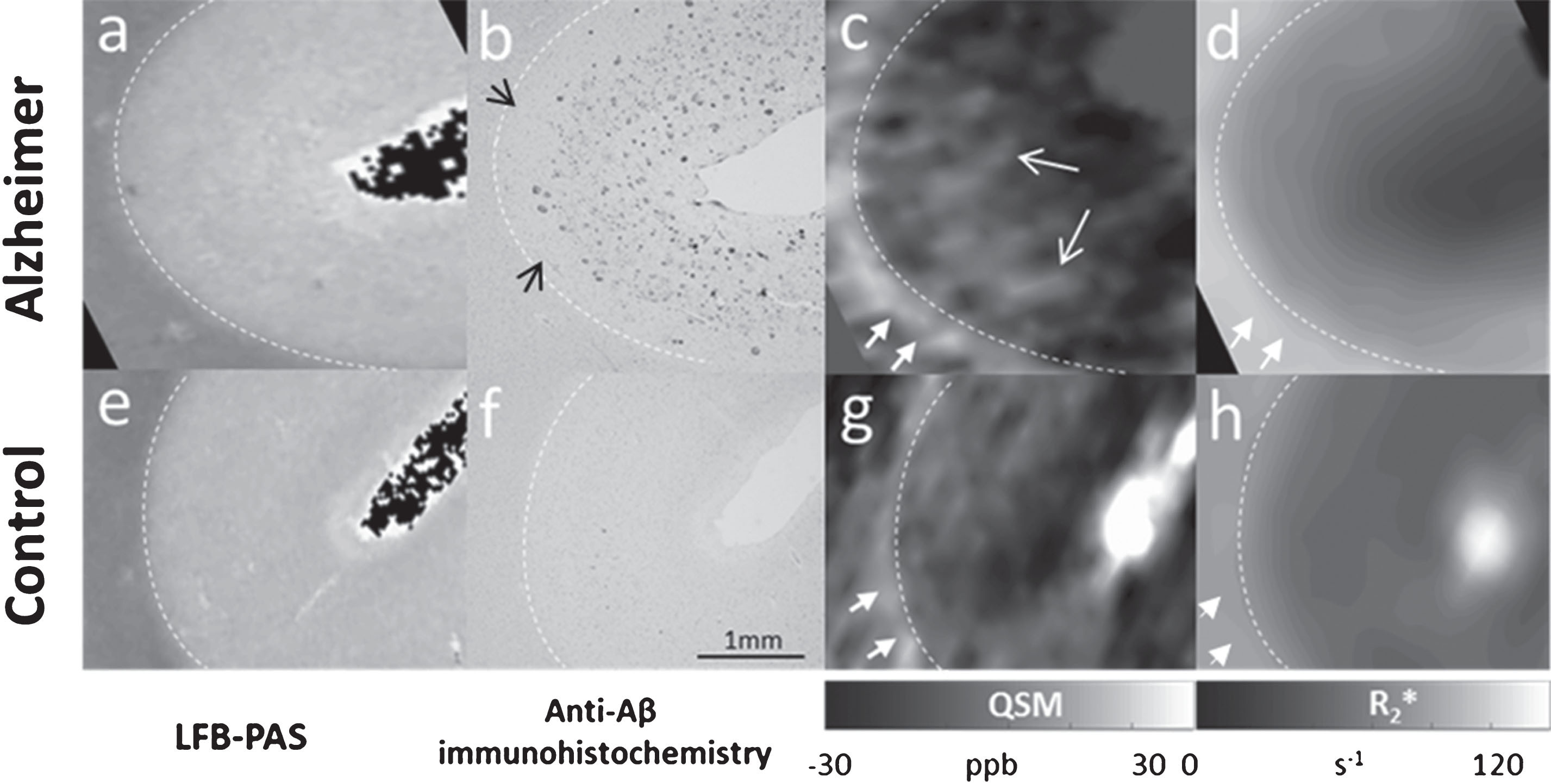
Comparison between histology (a, b, e, f) and ex vivo MRI at 9.4T (c, d, g, h). LFB-PAS staining and anti-Aβ immunohistochemistry in the frontal cortex of an AD patient (a, b) and a matched HC (e, f). QSM and R₂* of the AD patient (c, d) and HC (g, h), obtained using voxel sizes of 132×132×610 μm³ and 375×375×1000 μm³, respectively. GM/WM border, based on the LFB-PAS staining, is indicated by the dashed white lines in all the images. Amyloid plaques were detected in the Aβ stain of the AD patient within the cortex (b), while no plaques were detected in the cortex of HC (f). Hyperintense spots detected by QSM in the cortex of the patient (c, open white arrows) may likely correspond to the plaques in the Aβ stain (b). A clear hyperintense pattern was also observed in the susceptibility maps of both AD and HC in the superficial WM (c, g, filled white arrows), reaching susceptibility values up to 30 ppb in AD and 20 ppb in HC, respectively. The same pattern, with values of up to 100 s^–¹ in AD and 80 s^–¹ in HC, was also detected in the R₂*-maps, although in less details due to the coarser voxel size used (d, h, white arrows).

Fig.3

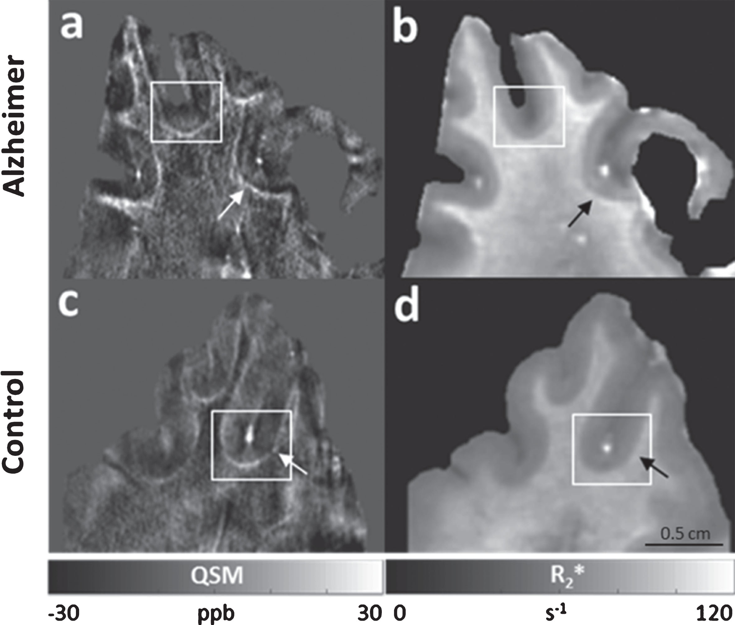
Overview image of the ex vivo MRI at 9.4T. QSM (a, c) and R₂* (b, d) of an AD patient (a, b) and a matched HC (c, d) obtained using voxel sizes of 132×132×610 μm³ and 375×375×1000 μm³, respectively. A distinct hyperintense pattern in the superficial WM of both AD (a, b) and HC (c, d) could be observed in both QSM (a, c, white arrows) and R₂*-maps (b, d, black arrows). White boxes in a, b, c and d correspond to the MRI zoomed-in areas (c, d, g, h, respectively) in Fig. 2.

Quantitative R₂* and susceptibility maps at 14.1T

Similarly to the ex vivo results obtained at 9.4T we observed a clear pattern in the juxtacortical WM characterized by hyperintense effects, which were present in both R₂* (Fig. 4c, f, dashed black arrows) and QSM (Fig. 4a, b, d, e, dashed white arrows) in AD (Fig. 4a, b) and HC (Fig. 4d, e). Specifically, the effective transverse relaxation rate was 100 s^–¹ in the juxtacortical WM of HC and 120 s^–¹ in AD. In the same region we observed maximum susceptibility values of 40 ppb in AD (Fig. 4a, b) and 30 ppb in HC (Fig. 4d, e), at the spatial sampling of 50 (Fig. 4a, d) and 100 μm (Fig. 4b, e). A distinct contrast variation across the cortical depth was observed that distinguished the AD patient from the HC sample in both R₂* and susceptibility maps at each spatial resolution. Specifically, in the cortex of AD, both quantitative maps clearly indicated two main areas running tangential with the cortical surface: a predominantly paramagnetic band characterized by hyperintense effects, apparently extending from layer I to layer V, as pointed out in Fig. 4 (a, b, c, filled white arrows) and a diamagnetic band, characterized by strong hypointense effects, apparently corresponding to the deepest portion of the cortex (possibly layer VI) (Fig. 4a, b, c, open white arrows). These strong diamagnetic effects may contribute to the greater contrast observed in the GM/WM border in AD compared to HC. On the other hand, in the cortex of the HC, three bands could be detected: two diamagnetic bands in the superficial and deep layers of the cerebral cortex (Fig. 4d, e, f, open white arrowheads) and a paramagnetic band (Fig. 4d, e, f, filled white arrows) in the intermediate layers of the cortex. Compared to AD this intermediate paramagnetic band was identified as being less broad and less paramagnetic.

Fig.4

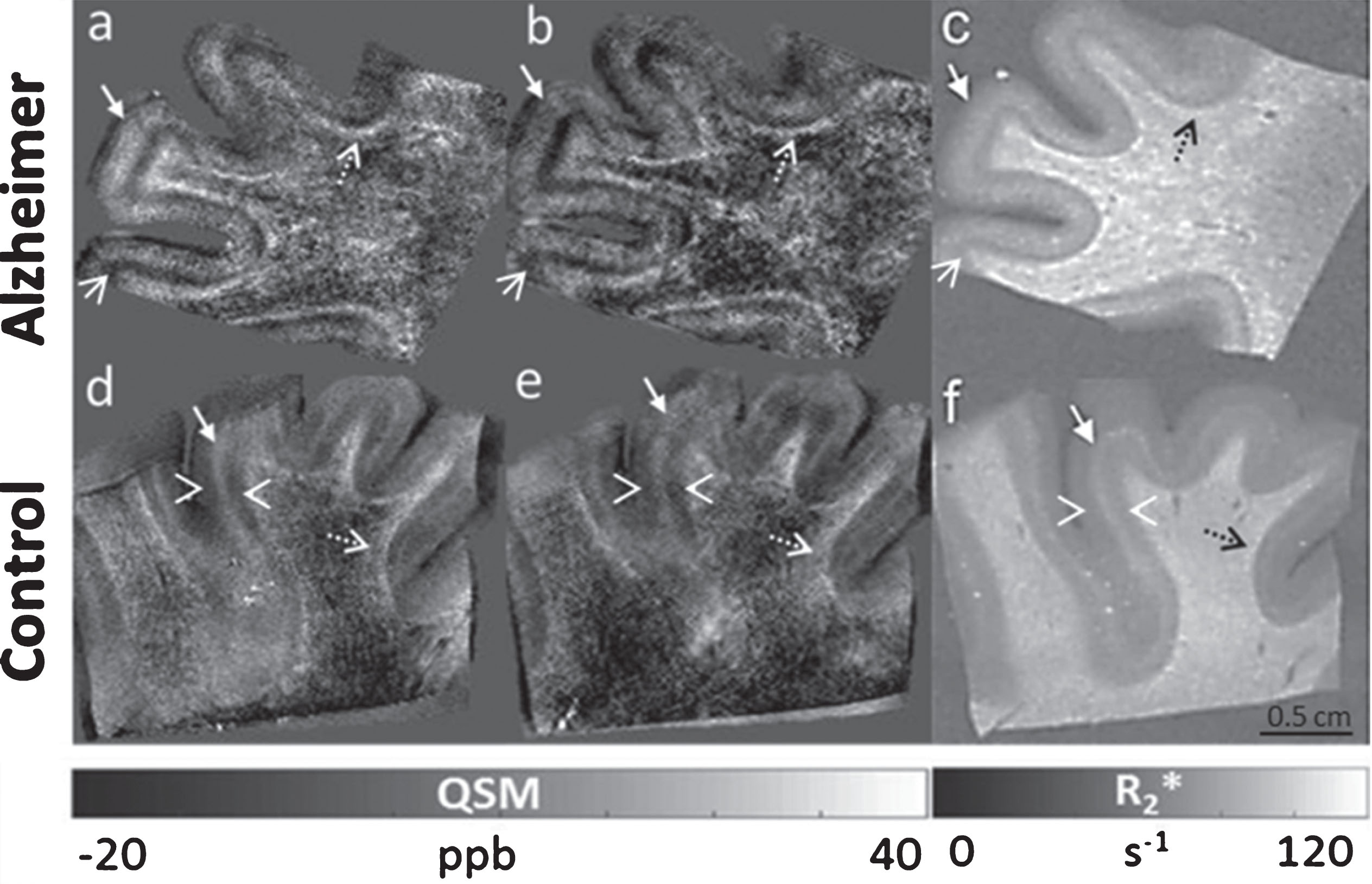
Ex vivo MRI at 14.1T, obtained from the frontal cortex of an AD patient and a matched HC. QSM (–20 to 40 ppb) of an AD patient (a, b) and a HC (d, e) obtained using an isotropic voxel size of 50 μm (a, d), and 100 μm³ (b, e), respectively. R₂*-maps (0–120 ms^–1) of AD (c) and HC (f), obtained using a voxel size of 100 μm isotropic. Similarly to the ex vivo results obtained at 9.4T a clear hyperintense pattern in the juxtacortical WM was observed in both R₂* (c, f, dashed black arrows) and QSM (a, b, d, e, dashed white arrows). Also, a distinct contrast variation across the cortical layers was detected in AD (a, b, c) compared to HC (d, e, f) in both R₂*(c, f) and QSM (a, b, d, e). Specifically, in the cortex of AD, both quantitative maps clearly indicated two main areas running tangential with the cortical surface: a predominantly paramagnetic band characterized by hyperintense effects apparently extending from layer I to layer V (a, b, c, filled white arrows) and a diamagnetic band characterized by strong hypointense effects, apparently corresponding to the deepest portion of the cortex (possibly layer VI) (a, b, c, open white arrows). In the cortex of the HC, three bands could be detected: two diamagnetic bands in the superficial and deep layers of the cerebral cortex (d, e, f, open white arrowheads) and a paramagnetic band (d, e, f, filled white arrows) in the intermediate layers of the cortex. Compared to AD this intermediate paramagnetic band was identified as being less broad and less paramagnetic.

Comparison of high resolution 14.1T ex vivo susceptibility maps with histology

Pushing further the limits of MRI to voxel sizes of 37 μm isotropic confirmed and showed in more detail the presence in the susceptibility maps of a distinctive pattern across the cortical depth of the AD patient when compared to the HC. Specifically, Fig. 5 shows two main bands in the cortex of AD (c and m, open white arrowheads (paramagnetic band) and filled white arrows (diamagnetic band), respectively), and three bands in the cortex of HC (f and s, filled white arrows (diamagnetic bands) and open white arrows (paramagnetic band), respectively). Significantly, dotted paramagnetic effects were observed in the cortex of the AD patient (Fig. 5c, m, open white arrowheads) at this spatial resolution. These effects resembled the Aβ plaques distribution found in the histological sections with regard to their shape and the cortical layers in which they were localized (Fig. 5b, i, open black arrowheads). In contrast, no plaques were revealed in the cortex of the HC with Aβ immunohistochemistry (Fig. 5e, dashed box, and 5q), and, accordingly, no paramagnetic effects could be observed in QSM in the cortex of the HC, as evidenced in Fig. 5 (f, s). Also, in the juxtacortical WM the same pattern as that observed using 100 and 50 μm isotropic voxels was detected in the QSM of both AD (Fig. 5c, n, white arrowheads) and in HC (Fig. 5f, t, dashed white arrows), reaching values up to 30 ppb and 20 ppb in AD and HC, respectively. In corresponding WM areas in the AD patient, the histological sections revealed the presence of Aβ deposits (Fig. 5b, l, filled black arrowheads). In accordance with these results, a previous study has reported increased intensity in iron stained sections in the juxtacortical WM in HC [65], likely reflecting vessels [66, 67]. These observations are concordant with our detected paramagnetic signal in the HC.

Fig.5

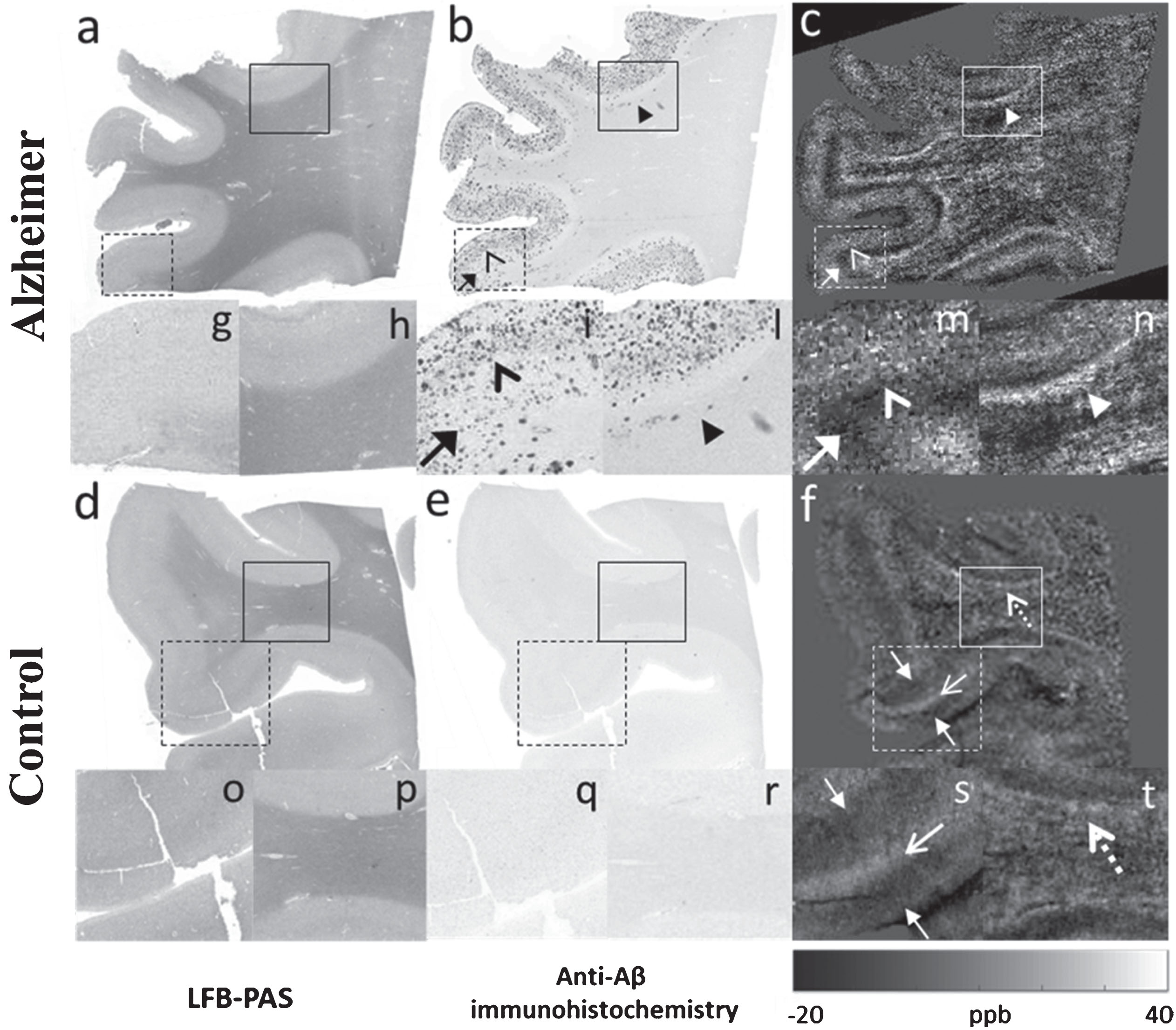
Comparison between ex vivo MRI at 14.1T using isotropic voxel size of 37 μm and histology. LFB-PAS staining (a, d), anti-Aβ immunohistochemistry (b, e), and QSM (c, f) from the frontal cortex of an AD (a, b, c) and of a matched HC (d, e, f). (g), (i), and (m), zoomed-in areas corresponding to the dashed boxes in (a), (b), and (c). (h), (l), and (n), zoomed-in areas corresponding to the boxes in (a), (b), and (c). (o), (q), and (s), zoomed-in areas corresponding to the dashed boxes in (d), (e), and (f). (p), (r), and (t), zoomed-in areas corresponding to the boxes in (d), (e), and (f). Dotted paramagnetic effects were observed in the cortex of the AD patient in the susceptibility maps (m, open white arrowhead). These effects resembled the Aβ plaques distribution found in the histological sections with regard to their shape and the cortical layers in which they were localized (i, open black arrowhead). No plaques were revealed in the cortex of the HC with Aβ immunohistochemistry (q) and, accordingly, no paramagnetic effects could be observed in QSM in the cortex of the HC (s). The juxtacortical WM showed the same pattern as that observed using 100 and 50 μm isotropic voxels in the QSM of both AD (n, white arrowhead) and in HC (t, dashed white arrow), reaching values up to 40 ppb and 30 ppb in AD and HC, respectively.

Aβ load detection

From the evaluation of the immunohistochemical data, we found an Aβ plaque fraction of 0.15 (% of the cortical area), which is in line with previously published reports on mice models [28]. Dependent on the QSM cutoff value and the image voxel size, this expected amount of plaque load could be observed in QSM. Figure 6 shows the Aβ load detected by QSM at different cutoffs in AD (red) and HC (blue), ex vivo (a–d) and in vivo (e) at 14.1T (a–c) and at 9.4T (d-e). (please refer to the online version for coloured figures). The plaque fraction (PL) detected by Aβ-stained histological sections within the cortex of AD is also shown (black horizontal line). The fraction of QSM-detected paramagnetic voxels decreased non-linearly with the cutoff values. The plaque load distributions of the two samples were consistently different (KS, p < 0.05), with higher apparent Aβ load detected in AD than in HC, despite decreasing spatial resolutions. To be thorough, we also investigated possible differences between the Aβ load distributions at 9.4T in vivo. The same trend was found at this coarser spatial resolution. The intersection of the QSM-based Aβ load and the fraction of plaques determined from the Aβ stain varied with voxel size and tissue (ex vivo or in vivo). For the ex vivo samples, using voxel sizes of 100 μm or larger, the QSM-detected Aβ load never reached the values observed by the Aβ stain when selecting cutoffs equal or higher than 10 ppb (Fig. 6c, d, red curve). If even lower cutoffs had been chosen, the risk of false positives, indicated by the curve obtained in HC, would also have increased. This observation from the same sample measured at 14.1T (a–c) could be confirmed for the ex vivo sample at 9.4T (d). In vivo, the detection of the expected Aβ load corresponded to a QSM cutoff of 20 ppb (Fig. 6e) as generally greater QSM values were observed in vivo than ex vivo. The susceptibility maps corresponding to the plaque load at the 10 ppb cutoff within the cerebral cortex clearly evidenced the spatial distribution of the plaques (Fig. 6, bottom row) and were closely similar to the plaque distribution already noted in the Aβ stained sections (Fig. 5b). Most plaques were located in the intermediate layers of the cerebral cortex, while the deeper layers were devoid of paramagnetic effects. However, a clear distinction of this cortical pattern was mainly possible using high resolution techniques at 14T. In the QSM obtained using a clinical imaging protocol ex vivo at 9.4T this pattern was less evident whereas in vivo it was not possible to observe it.

Fig.6

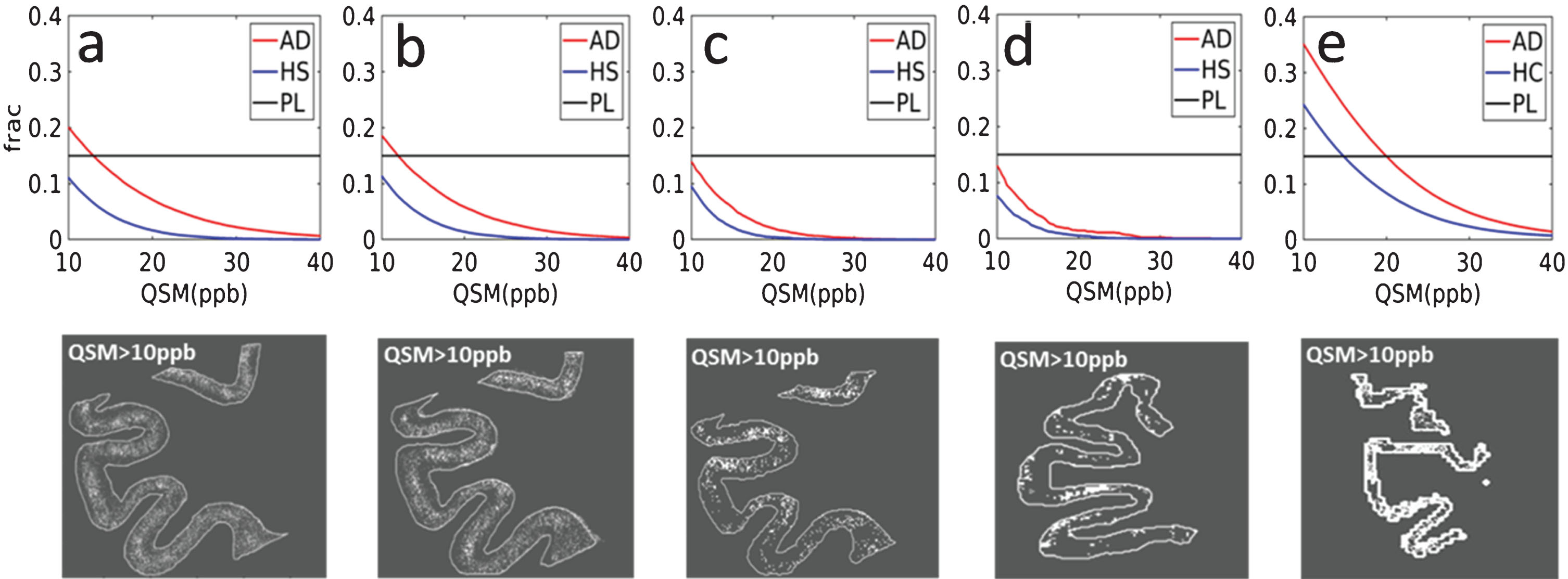
Fraction (frac) of paramagnetic pixels detected by QSM in the cortex of an AD patient (red) and a HC (blue) samples, at different cutoff values for QSM at 14.1T (a–c) at 37 μm (a), 50 μm (b), and 100 μm (c) isotropic voxel size and using a clinical imaging protocol at 9.4T with 132×132×610 μm³ voxels (d). In vivo results using the same QSM method at 9.4T (e). The fraction of plaques (PL) in the cortex of the AD sample obtained from Aβ-stained histological slice is also shown (horizontal black line). In the bottom row susceptibility maps thresholded at 10 ppb, corresponding to the Aβ plaque load in (a–e), are shown. A consistent difference between AD and HC was found in vivo and ex vivo (at each spatial resolution). Load detection ability, ex vivo, showed a decrease in performance as a function of the spatial resolution, being lower for voxel sizes of 100 μm isotropic and 132×132×610 μm³ (c, d), in comparison with 50 and 37 μm isotropic (a, b). The apparent Aβ load detected in vivo (e) was higher compared to the ex vivo measurements at the same field strength and spatial resolution.

Histogram analysis of QSM values at 14.1T

Analyses of histograms of QSM values measured within the GM of AD and HC ex vivo at 14.1T showed a general broadening of the curve in AD compared to HC, at each spatial resolution (Fig. 7). Figure 7 shows normalized histograms in the cortex of the AD patient (red) and the HC (blue), at each spatial resolution at 14.1T. Broader curves were obtained for isotropic voxel size of 37 and 50 μm (a, b) compared to 100 μm (c), thus suggesting a higher capacity to detect both paramagnetic and diamagnetic effects at finer sampling. Furthermore, the AD curves showed an overall shift towards diamagnetic values compared to HC when using isotropic voxel sizes of 100 μm (c). The vertical dotted black line shows the threshold at 10 ppb, corresponding to the binary plaque load images in the bottom row of Fig. 6.

Fig.7

Normalized histograms within the cortex of AD patient (red) and HC (blue) at 37 (a), 50 (b). and 100 μm (c) isotropic voxel sizes, at 14.1T. In general, a greater range of both diamagnetic and paramagnetic QSM values were observed in AD than in HC at each spatial resolution. Broader distribution curves at 37 and 50 μm isotropic voxel sizes indicate a higher ability to detect both paramagnetic and diamagnetic effects at higher spatial resolutions. For a greater isotropic voxel size of 100 μm, a diamagnetic shift towards lower QSM values was observed for the AD patient. The vertical dotted black line shows the threshold at 10 ppb used for the binary spatial maps in the bottom row of Fig. 6.

Beyond exploring the cortical layers, we further analyzed the magnetic properties of the WM. However, no visible differences between AD and HC were found at any of the investigated spatial resolutions suggesting that only alterations across the cortical layers may be taken into account in order to differentiate between AD and HC, and hence, that QSM values in the WM may be used as an internal reference region in future clinical studies.

DISCUSSION AND CONCLUSION

We found a distinctive cortical pattern in AD patients compared to HC in agreement with previous in vivo results at 7T using non-quantitative MRI techniques [32]. This observation was confirmed by ex vivo measurements at both 9.4T and 14.1T. We observed a close similarity between the signal changes detected by QSM in the cortex of the AD sample at 14.1T and the spatial distribution of Aβ plaques in the histological sections of the same specimen. Finally, we found that the cortical layers with a high plaque load can be detected using QSM at a cutoff between 10 and 20 ppb ex vivo and 20 ppb in vivo.

Our in vivo findings are in line with previous results obtained using GRE phase images at 7T [32]. Extending upon these studies we used quantitative R₂* and QSM and we found an enhanced contrast between the GM and WM in AD patients in comparison with HC at 9.4T. This contrast originated from a strong difference in the magnetic susceptibility and in the effective transverse relaxation rate between GM and WM, and it was higher in AD than in HC. The use of QSM in this work offered the additional advantage to separate between paramagnetic (e.g., iron) and diamagnetic (e.g., myelin and Aβ protein [30]) sources, since the technique removes the non-local and orientation-dependent effects of the GRE phase signal and provides a measure that more closely reflects the underlying tissue microstructure compared to other techniques. In previous studies, QSM has been found to be increased in the cortex of AD patients compared to HC at 3T [36] and at 7T [29], as well as in the globus pallidus [29], precuneus, and hippocampus [38]. Nevertheless, these studies were burdened by low spatial resolutions and enabled only a relatively coarse localization of the regions affected by the Aβ load, since voxel sizes from 0.7 mm isotropic were used. Due to recent advancements in hardware and efficient spatial encoding at 9.4T in this study we were able to push the image resolution down to 132×132×610 μm³ in vivo. In line with the previously mentioned studies, we could find a global effect distinguishing AD from HC. However, from our data we are still not able to conclude with certainty that it is possible to detect in vivo highly localized paramagnetic effects corresponding to the Aβ deposits.

These in vivo preliminary results in AD patients at 9.4T deserve further investigation to fully develop clinically compatible methods. Such methods should also take into account effects related to phase fluctuations in the brain caused by physiological noise (e.g., breathing) and motion (e.g., swallowing or arms moving) within the field, especially in patients, besides possible system instabilities causing field fluctuations affecting the measures. A navigator echoes approach has been proposed to better estimate the spatio-temporal magnetic field distribution during large B₀-fluctuations for GRE-based MRI in 2D [68, 69]. Such methods may possibly enhance the visibility of Aβ deposits in vivo, since data blurring will likely be diminished. The implementation of such quantitative approaches will likely improve the quality of in vivo data and their use may therefore be extended to a broader patient population and elderly people. We are currently undertaking actions in this direction and have obtained promising results for a navigator echo-based approach in 3D [70]. On the other hand, the detectability of the effects of Aβ plaques would still be hampered by the large voxel sizes achievable in vivo, as it is more than 100-fold bigger than the plaques diameter (20–160 μm). Thus, in order to better understand the source of the MRI contrast in vivo, we measured postmortem samples using the same measurement protocol used for patient studies at 9.4T, and validated our observations by histology.

The ex vivo susceptibility maps obtained at 9.4T with our clinical protocol showed some point shaped regions with paramagnetic effects in the cortex of AD, but less so in HC tissue. These regions corresponded to areas in the cortex of AD where plaques were detected by the Aβ stain in the histological section of the same specimen. However, at the spatial resolution used for the in vivo protocol single plaques could not be distinguished with certainty, thus confirming an inherent detection limit for single plaques in vivo. A paramagnetic increase in QSM was also observed in the juxtacortical WM of both the AD patient and HC in the susceptibility maps. This effect is consistent with a strong contrast observed at 7T in R₂*-maps and susceptibility weighted images (SWI) of healthy subjects [65] likely due to the presence of short vessels in the U-fibers [66, 67], located in a 3-4 mm thick band of WM immediately beneath the cortex. In our data we found that the paramagnetic effect in this area was greater in the AD patient compared to the HC, suggesting that other factors may influence the detected QSM values. To better understand the MRI contrast obtained at 9.4T ex vivo, we further validated our measurements of postmortem samples using higher magnetic field strength (14.1T), where finer sampling is feasible in view of the increased signal. Morover, increased magnetic field also causes higher values of the R₂* and greater effects of the local magnetic susceptibility which can facilitate the observation of subtle differences in the tissue.

The histopathological basis of MRI contrast changes associated with Aβ plaques has been previously investigated in human and animal specimens ex-vivo at 7T using 60 μm thick histological sections and a fine in-plane spatial sampling of 45 μm [22, 23]. By comparing T₂*-weighted images with histological sections stained with the iron-sensitive diaminobenzidine (DAB)-enhanced Perl’s stain and Aβ immunohistochemistry, before and after iron chelation, the authors suggested that both the high focal iron concentration, the highly compact fibrillar Aβ and the morphology of the deposits per se may explain T₂* shortening, since hypointensities corresponding to Aβ plaques could still be detected after iron chelation. However, T₂* weighting is not a quantitative method, and it cannot distinguish between diamagnetic (Aβ protein) and paramagnetic sources (iron). Therefore, the observed signal after chelation could have been caused by the presence of the Aβ protein itself, being a diamagnetic source, independently of its morphology. Moreover, due to the inability to distinguish between the two contributions, T₂*-weighted images cannot provide a refined measure of the actual microstructure of the tissue. In the present work we therefore used quantitative measures, such as QSM and R₂*, to complement such observations.

At 14.1T we could confirm the observations made using clinical measurement protocols at 9.4T. In addition to the strong paramagnetic effects in the intermediate layers of the cortex, we observed paramagnetic values in the juxtacortical WM of both AD and HC. The difference in the apparent layering pattern across the cortical depth between AD and HC was clear in R₂*-maps using an isotropic voxel size of 100 μm, and in the susceptibility maps using 100 and 50 μm isotropic voxel sizes, respectively, showing a predominantly paramagnetic cortex in AD compared to HC, and local paramagnetic hyperintensities that were more frequent in the intermediate layers of the cerebral cortex.

At even higher spatial resolution (37 μm isotropic) we found a close similarity between the localization of the paramagnetic spots detected by QSM in the cortex of the AD patient and the distribution pattern of Aβ plaques, by comparing the results of QSM and Aβ immunohistochemistry, although a direct one-to-one correlation of single Aβ plaques to MR signals could not be achieved. The presence of the plaques, therefore, could explain the distinct cortical (para- and diamagnetic) bands observed in AD cortex compared to HC. The strong diamagnetic effect in the deepest layers of the cortex of AD, close to the GM/WM border, corresponded to an area where the Aβ stain showed absence of plaques, but no increase in the myelin stain (LFB-PAS) was found. Although this diamagnetic effect was also present in HC, the values in AD outsized the values observed in healthy tissue. Previous reports show that this cortical area is dominated by tau pathology [71, 72]. The slight deposition of Aβ in the superficial WM of AD revealed by the stain and the diamagnetic band in the deepest cortical layers, could explain the higher enhanced contrast between GM and WM we observed in both R₂* and QSM of AD, at each spatial resolution. The increased signal detected by QSM and R₂*-maps in the juxtacortical WM of both AD and HC is likely due to the presence of vessels [66, 67], but we could show that this effect can be further enhanced in the presence of Aβ deposits. Furthermore, this contrast is stronger in QSM than in the R₂*-map, and could also reflect demyelination processes in the superficial WM of AD patients [73, 74]. Hereby, a lower contribution from the diamagnetic susceptibility to the global effect will lead to an increase of QSM and a reduction of R₂* values in the maps.

To develop clinically useful MRI-based biomarkers, quantitative analysis is desirable. Previous studies have quantified the Aβ load by using T₂*-weighted images in comparison with ¹¹C-PIB PET in mice models [28]. The authors found a linear correlation between ¹¹C-PIB PET and T₂*-weighted Aβ-positive fractions in thalamus, hippocampus, temporo parietal, and frontal cortex. In the present study we assessed the Aβ load using QSM in comparison with the plaques load obtained from histology. We found that the cortical layers with a high plaque load can be detected using QSM at a cutoff between 10 and 20 ppb ex vivo, and 20 ppb in vivo. Notice that, in ex vivo measurements, higher cutoff was required to detect the Aβ load at higher spatial resolutions, being 15 ppb for 37 μm³ and lower than 10 ppb for 100 μm³, respectively. This could be due to the presence of partial volume effects that mask the dominantly paramagnetic effect of the Aβ deposits, when larger voxel sizes are used. After application of the cutoff, we were able to obtain mask images that closely matched the distribution of Aβ in histological sections, with a predominant localization of the plaques along the intermediate portion of the cerebral cortex and absence of paramagnetic effects in the deepest cortical layers. The apparent Aβ load detected in vivo at 9.4T was higher compared to the ex vivo measurements at the same field strength and spatial resolution. This is possibly due to the loss of iron in ex vivo samples, which could occur during the fixation process. Furthermore, venous blood could significantly contribute to the MRI contrast in in vivo measurements. Since perfusion differences between AD and healthy subjects do exist, the influence of such factors on the in vivo QSM results deserve further investigations in future studies. In addition, in view of the common QSM reference value we could directly compare the QSM values observed in the two samples at different voxel sizes. Similarly, we estimated the difference between the Aβ load curves and the histograms of the single-case AD and HC samples. A difference between the Aβ load distribution of the two samples was consistently found, with higher values in AD than in HC, at each spatial resolution, at both 9.4T and 14.1T. Likewise, we also found a difference for the in vivo Aβ load distributions. Also, a difference between the histograms of the AD and the HC samples was found at each voxel size at 14.1T.

Interestingly, we not only detected paramagnetic effects linked with Aβ deposits in the ex vivo specimens at 14.1T, as evidenced by the QSM obtained at different voxel sizes in AD, but we also showed an increase in the diamagnetic effects through analysis of the distribution of QSM values in histograms within the cortex. The QSM distributions of AD and HC were consistently different at each spatial resolution. At the finest sampling the distribution was roughly symmetric around 0 ppb. Interestingly, with increasing voxel size, the diamagnetic effect outsized the paramagnetic effects. One explanation of this phenomenon is that partial volume effects diminish the iron-related paramagnetic effect. Adding on to this, the diamagnetic effects in the deeper located parts of the cortex may dominate the total signal when larger voxel sizes are used thus explaining previous reports concerning such effects [30].

Our study was restricted by some limitations. First of all, obtaining QSM by ex vivo MRI can be cumbersome. Thin histological sections pose challenges as the mathematical algorithms used for QSM computation generally depend on 3D information in Fourier space. On the other hand, it is possible to achieve such results for thicker specimens, as we showed in the present study. Also, a big effort was required for the spatial registration of the 3D-MRI volume to the 2D histological slice and no perfect match was reached between MRI images and histology. Although an easier, faster and accurate registration could have been provided by the use of a histological coil, leading to an easier 2D-2D registration, a 3D volume was necessary to perform QSM, which strongly depends on both the slice thickness and coverage [75]. Therefore, a volume coil had to be used. Nevertheless, we deemed the spatial registration to be sufficient to perform quantitative analysis and to evaluate the relation between MRI and histology. Another inherent caveat of QSM is the absence of an absolute reference value. We circumvented this issue by acquiring and processing MRI data of both specimens (AD and HC) together. This procedure ensured that the QSM values in the two samples could be directly compared, thus allowing a more precise evaluation of pathology induced differences, including overall shifts in magnetic susceptibility. Besides that, the current approach used to remove the background field for the calculation of QSM ex vivo could not eliminate the presence of false positives in the ex vivo maps, which may explain the apparent Aβ load detected by QSM in the cortex of the HC, which was not confirmed through histology, as no Aβ deposits were detected in the histological stain of the HC.

This study clarified that UHF quantitative MRI provides optimized spatial localization of the affected areas by Aβ deposits in the cortex of AD, in contrast to the coarse localization provided by PiB-PET. We further demonstrated that R₂*-maps and QSM at UHF are an indirect measure of the spatial distribution of the Aβ deposits in specific layers of the cerebral cortex, since these techniques can detect the prevalent effects directly related to Aβ deposits in AD patients, besides possible alterations in tissue microstructure across the cortical layers.

We also showed the limitations posed in terms of quantifying the plaque load when going to imaging parameters achievable in vivo. Ex vivo MRI measurements proved that higher spatial resolutions are necessary to directly observe these dominant effects and, therefore, to precisely estimate the plaque load. Interestingly, we found a consistent difference between the Aβ load distributions of the AD and the HC samples, at each spatial resolution and at each field strength. This difference was also observed at the coarsely sampled in vivo data.

Furthermore, analyses of histogram showed that the diamagnetic properties of the cortex could provide a further means to distinguish AD patients from HC using voxel sizes from (100 μm)³. Layer-dependent microstructural changes should also be taken into account for AD classification and as biomarkers of AD.

In conclusion, our findings confirm that it is possible to differentiate between AD and HC in vivo at UHF by achieving very high spatial resolutions and by detecting changes in the cortex of AD arising from Aβ plaques. In addition, this study provided a method for detecting these changes independently of the acquisition protocol and the orientation of the object with respect to the static field.

Finally, we provided a quantitative method to quantify the amyloid plaque load in AD patients at UHF non-invasively. Future work will focus on studying a larger cohort to generalize our findings to a broader AD population and other target brain areas.

To our knowledge, and in line with a recent review paper [76], this is the first time QSM is used to investigate AD patients at 9.4T, as well as human AD and HC samples both at 9.4T and 14.1T in comparison with histology. Furthermore, for the first time a direct comparison of QSM values between AD and HC could be achieved, ex vivo, since the samples were acquired and processed simultaneously, thus allowing an unbiased comparison between them.

The availability of a potentially non-invasive technique capable to detect, locally, the areas affected by Aβ plaques in preclinical stages of AD is of crucial importance, since it would allow the patient to be treated before the clinical onset of the disease many years in advance.

Footnotes

ACKNOWLEDGMENTS

We gratefully acknowledge the Alzheimer Förder Initiative eV, Germany Grant #DE-15036 and EU-LACH Grant #16/T01-0118 for supporting this work.

Authors’ disclosures available online ().

References

Selkoe

(1991) Amyloid protein and Alzheimer’s disease. Sci Am 265, 68–71, 74-66, 78.

Hardy

, Higgins

(1992) Alzheimer’s disease: The amyloid cascade hypothesis. Science 256, 184–185.

Jack

Jr , Knopman

, Jagust

, Shaw

, Aisen

, Weiner

, Petersen

, Trojanowski

(2010) Hypothetical model of dynamic biomarkers of the Alzheimer’s pathological cascade. Lancet Neurol 9, 119–128.

Hardy

, Selkoe

(2002) The amyloid hypothesis of Alzheimer’s disease: Progress and problems on the road to therapeutics. Science 297, 353–356.

Hardy

, Allsop

(1991) Amyloid deposition as the central event in the aetiology of Alzheimer’s disease. Trends Pharmacol Sci 12, 383–388.

Bateman

, Xiong

, Benzinger

, Fagan

, Goate

, Fox

, Marcus

, Cairns

, Xie

, Blazey

, Holtzman

, Santacruz

, Buckles

, Oliver

, Moulder

, Aisen

, Ghetti

, Klunk

, McDade

, Martins

, Masters

, Mayeux

, Ringman

, Rossor

, Schofield

, Sperling

, Salloway

, Morris

, Dominantly Inherited Alzheimer Network (2012) Clinical and biomarker changes in dominantly inherited Alzheimer’s disease. N Engl J Med 367, 795–804.

Benzinger

, Blazey

, Jack

Jr , Koeppe

, Su

, Xiong

, Raichle

, Snyder

, Ances

, Bateman

, Cairns

, Fagan

, Goate

, Marcus

, Aisen

, Christensen

, Ercole

, Hornbeck

, Farrar

, Aldea

, Jasielec

, Owen

, Xie

, Mayeux

, Brickman

, McDade

, Klunk

, Mathis

, Ringman

, Thompson

, Ghetti

, Saykin

, Sperling

, Johnson

, Salloway

, Correia

, Schofield

, Masters

, Rowe

, Villemagne

, Martins

, Ourselin

, Rossor

, Fox

, Cash

, Weiner

, Holtzman

, Buckles

, Moulder

, Morris

(2013) Regional variability of imaging biomarkers in autosomal dominant Alzheimer’s disease. Proc Natl Acad Sci U S A 110, E4502–4509.

Sperling

, Jack

Jr , Black

, Frosch

, Greenberg

, Hyman

, Scheltens

, Carrillo

, Thies

, Bednar

, Black

, Brashear

, Grundman

, Siemers

, Feldman

, Schindler

(2011) Amyloid-related imaging abnormalities in amyloid-modifying therapeutic trials: Recommendations from the Alzheimer’s Association Research Roundtable Workgroup. Alzheimers Dement 7, 367–385.

Fagan

, Csernansky

, Morris

, Holtzman

(2005) The search for antecedent biomarkers of Alzheimer’s disease. J Alzheimers Dis 8, 347–358.

10.

Reiman

, Langbaum

, Tariot

, Lopera

, Bateman

, Morris

, Sperling

, Aisen

, Roses

, Welsh-Bohmer

, Carrillo

, Weninger

(2016) CAP–advancing the evaluation of preclinical Alzheimer disease treatments. Nat Rev Neurol 12, 56–61.

11.

Bacskai

, Frosch

, Freeman

, Raymond

, Augustinack

, Johnson

, Irizarry

, Klunk

, Mathis

, Dekosky

, Greenberg

, Hyman

, Growdon

(2007) Molecular imaging with Pittsburgh Compound B confirmed at autopsy: A case report. Arch Neurol 64, 431–434.

12.

Driscoll

, Troncoso

, Rudow

, Sojkova

, Pletnikova

, Zhou

, Kraut

, Ferrucci

, Mathis

, Klunk

, O’Brien

, Davatzikos

, Wong

, Resnick

(2012) Correspondence between in vivo (11)C-PiB-PET amyloid imaging and postmortem, region-matched assessment of plaques. Acta Neuropathol 124, 823–831.

13.

Johnson

, Gregas

, Becker

, Kinnecom

, Salat

, Moran

, Smith

, Rosand

, Rentz

, Klunk

, Mathis

, Price

, Dekosky

, Fischman

, Greenberg

(2007) Imaging of amyloid burden and distribution in cerebral amyloid angiopathy. Ann Neurol 62, 229–234.

14.

Kantarci

, Ferman

, Boeve

, Weigand

, Przybelski

, Vemuri

, Murray

, Senjem

, Smith

, Knopman

, Petersen

, Jack

Jr , Parisi

, Dickson

(2012) Focal atrophy on MRI and neuropathologic classification of dementia with Lewy bodies. Neurology 79, 553–560.

15.

Klunk

, Engler

, Nordberg

, Wang

, Blomqvist

, Holt

, Bergstrom

, Savitcheva

, Huang

, Estrada

, Ausen

, Debnath

, Barletta

, Price

, Sandell

, Lopresti

, Wall

, Koivisto

, Antoni

, Mathis

, Langstrom

(2004) Imaging brain amyloid in Alzheimer’s disease with Pittsburgh Compound-B. Ann Neurol 55, 306–319.

16.

Lockhart

, Lamb

, Osredkar

, Sue

, Joyce

, Ye

, Libri

, Leppert

, Beach

(2007) PIB is a non-specific imaging marker of amyloid-beta (Abeta) peptide-related cerebral amyloidosis. Brain 130, 2607–2615.

17.

Murray

, Lowe

, Graff-Radford

, Liesinger

, Cannon

, Przybelski

, Rawal

, Parisi

, Petersen

, Kantarci

, Ross

, Duara

, Knopman

, Jack

Jr , Dickson

(2015) Clinicopathologic and 11C-Pittsburgh compound B implications of Thal amyloid phase across the Alzheimer’s disease spectrum. Brain 138, 1370–1381.

18.

Sojkova

, Driscoll

, Iacono

, Zhou

, Codispoti

, Kraut

, Ferrucci

, Pletnikova

, Mathis

, Klunk

, O’Brien

, Wong

, Troncoso

, Resnick

(2011) In vivo fibrillar beta-amyloid detected using [11C]PiB positron emission tomography and neuropathologic assessment in older adults. Arch Neurol 68, 232–240.

19.

Ikonomovic

, Klunk

, Abrahamson

, Mathis

, Price

, Tsopelas

, Lopresti

, Ziolko

, Bi

, Paljug

, Debnath

, Hope

, Isanski

, Hamilton

, DeKosky

(2008) Post-mortem correlates of in vivo PiB-PET amyloid imaging in a typical case of Alzheimer’s disease. Brain 131(Pt 6), 1630–1645.

20.

Niedowicz

, Beckett

, Matveev

, Weidner

, Baig

, Kryscio

, Mendiondo

, LeVine

3rd , Keller

, Murphy

(2012) Pittsburgh compound B and the postmortem diagnosis of Alzheimer disease. Ann Neurol 72, 564–570.

21.

Benveniste

, Einstein

, Kim

, Hulette

, Johnson

(1999) Detection of neuritic plaques in Alzheimer’s disease by magnetic resonance microscopy. Proc Natl Acad Sci U S A 96, 14079–14084.

22.

Meadowcroft

, Connor

, Smith

, Yang

(2009) MRI and histological analysis of beta-amyloid plaques in both human Alzheimer’s disease and APP/PS1 transgenic mice. J Magn Reson Imaging 29, 997–1007.

23.

Meadowcroft

, Peters

, Dewal

, Connor

, Yang

(2015) The effect of iron in MRI and transverse relaxation of amyloid-beta plaques in Alzheimer’s disease. NMR Biomed 28, 297–305.

24.

Nabuurs

, Natte

, de Ronde

, Hegeman-Kleinn

, Dijkstra

, van Duinen

, Webb

, Rozemuller

, van Buchem

, van der Weerd

(2013) MR microscopy of human amyloid-beta deposits: Characterization of parenchymal amyloid, diffuse plaques, and vascular amyloid. J Alzheimers Dis 34, 1037–1049.

25.

Wengenack

, Reyes

, Curran

, Borowski

, Lin

, Preboske

, Holasek

, Gilles

, Chamberlain

, Marjanska

, Jack

Jr , Garwood

, Poduslo

(2011) Regional differences in MRI detection of amyloid plaques in AD transgenic mouse brain. Neuroimage 54, 113–122.

26.

Chamberlain

, Reyes

, Curran

, Marjanska

, Wengenack

, Poduslo

, Garwood

, Jack

Jr (2009) Comparison of amyloid plaque contrast generated by T2-weighted, T2*-weighted, and susceptibility-weighted imaging methods in transgenic mouse models of Alzheimer’s disease. Magn Reson Med 61, 1158–1164.

27.

Zhang

, Yarowsky

, Gordon

, Di Carlo

, Munireddy

, van Zijl

, Mori

(2004) Detection of amyloid plaques in mouse models of Alzheimer’s disease by magnetic resonance imaging. Magn Reson Med 51, 452–457.

28.

Maier

, Keller

, Bukala

, Bender

, Mannheim

, Brereton

, Galloway

, Pichler

(2015) Quantification of beta-amyloidosis and rCBF with dedicated PET, 7 T MR imaging, and high-resolution microscopic MR imaging at 16.4 T in APP23 mice. J Nucl Med 56, 1593–1599.

29.

Tiepolt

, Schafer

, Rullmann

, Roggenhofer

, Netherlands Brain

, Gertz

, Schroeter

, Patt

, Bazin

, Jochimsen

, Turner

, Sabri

, Barthel

(2018) Quantitative susceptibility mapping of amyloid-beta aggregates in Alzheimer’s disease with 7T MR. J Alzheimers Dis 64, 393–404.

30.

Gong

, Dibb

, Bulk

, van der Weerd

, Liu

(2019) Imaging beta amyloid aggregation and iron accumulation in Alzheimer’s disease using quantitative susceptibility mapping MRI. Neuroimage 191, 176–185.

31.

van Rooden

, Doan

, Versluis

, Goos

, Webb

, Oleksik

, van der Flier

, Scheltens

, Barkhof

, Weverling-Rynsburger

, Blauw

, Reiber

, van Buchem

, Milles

, van der Grond

(2015) 7T T(2)*-weighted magnetic resonance imaging reveals cortical phase differences between early- and late-onset Alzheimer’s disease. Neurobiol Aging 36, 20–26.

32.

van Rooden

, Versluis

, Liem

, Milles

, Maier

, Oleksik

, Webb

, van Buchem

, van der Grond

(2014) Cortical phase changes in Alzheimer’s disease at 7T MRI: A novel imaging marker. Alzheimers Dement 10, e19–26.

33.

Bulk

, Abdelmoula

, Nabuurs

RJA

, van der Graaf

, Mulders

CWH

, Mulder

, Jost

, Koster

, van Buchem

, Natte

, Dijkstra

, van der Weerd

(2018) Postmortem MRI and histology demonstrate differential iron accumulation and cortical myelin organization in early- and late-onset Alzheimer’s disease. Neurobiol Aging 62, 231–242.

34.

Lee

, Shmueli

, Fukunaga

, van Gelderen

, Merkle

, Silva

, Duyn

(2010) Sensitivity of MRI resonance frequency to the orientation of brain tissue microstructure. Proc Natl Acad Sci U S A 107, 5130–5135.

35.

Stuber

, Morawski

, Schafer

, Labadie

, Wahnert

, Leuze

, Streicher

, Barapatre

, Reimann

, Geyer

, Spemann

, Turner

(2014) Myelin and iron concentration in the human brain: A quantitative study of MRI contrast. Neuroimage 93 Pt 1, 95–106 .

36.

Acosta-Cabronero

, Williams

, Cardenas-Blanco

, Arnold

, Lupson

, Nestor

(2013) In vivo quantitative susceptibility mapping (QSM) in Alzheimer’s disease. PLoS One 8, e81093.

37.

Zhao

, Raichle

, Wen

, Benzinger

, Fagan

, Hassenstab

, Vlassenko

, Luo

, Cairns

, Christensen

, Morris

, Yablonskiy

(2017) In vivo detection of microstructural correlates of brain pathology in preclinical and early Alzheimer Disease with magnetic resonance imaging. Neuroimage 148, 296–304.

38.

Kim

, Park

, Rhee

, Lee

, Ryu

, Rhee

, Lee

, Wang

, Jahng

(2017) Quantitative susceptibility mapping to evaluate the early stage of Alzheimer’s disease. Neuroimage Clin 16, 429–438.

39.

Liu

, Spincemaille

, de Rochefort

, Kressler

, Wang

(2009) Calculation of susceptibility through multiple orientation sampling (COSMOS): A method for conditioning the inverse problem from measured magnetic field map to susceptibility source image in MRI. Magn Reson Med 61, 196–204.

40.

Schweser

, Deistung

, Lehr

, Reichenbach

(2011) Quantitative imaging of intrinsic magnetic tissue properties using MRI signal phase: An approach to in vivo brain iron metabolism? Neuroimage 54, 2789–2807.

41.

Shmueli

, de Zwart

, van Gelderen

, Li

, Dodd

, Duyn

(2009) Magnetic susceptibility mapping of brain tissue in vivo using MRI phase data. Magn Reson Med 62, 1510–1522.

42.

Wharton

, Bowtell

(2010) Whole-brain susceptibility mapping at high field: A comparison of multiple- and single-orientation methods. Neuroimage 53, 515–525.

43.

Antharam

, Collingwood

, Bullivant

, Davidson

, Chandra

, Mikhaylova

, Finnegan

, Batich

, Forder

, Dobson

(2012) High field magnetic resonance microscopy of the human hippocampus in Alzheimer’s disease: Quantitative imaging and correlation with iron. Neuroimage 59, 1249–1260.

44.

Bulk

, van der Weerd

, Breimer

, Lebedev

, Webb

, Goeman

, Ward

, Huber

, Oosterkamp

, Bossoni

(2018) Quantitative comparison of different iron forms in the temporal cortex of Alzheimer patients and control subjects. Sci Rep 8, 6898.

45.

Langkammer

, Schweser

, Krebs

, Deistung

, Goessler

, Scheurer

, Sommer

, Reishofer

, Yen

, Fazekas

, Ropele

, Reichenbach

(2012) Quantitative susceptibility mapping (QSM) as a means to measure brain iron? A post mortem validation study. Neuroimage 62, 1593–1599.

46.

, Wu

, Avram

, Liu

(2012) Magnetic susceptibility anisotropy of human brain in vivo and its molecular underpinnings. Neuroimage 59, 2088–2097.

47.

Liu

, Li

, Johnson

, Wu

(2011) High-field (9.4 T) MRI of brain dysmyelination by quantitative mapping of magnetic susceptibility. Neuroimage 56, 930–938.

48.

Liu

(2010) Susceptibility tensor imaging. Magn Reson Med 63, 1471–1477.

49.

Langkammer

, Krebs

, Goessler

, Scheurer

, Ebner

, Yen

, Fazekas

, Ropele

(2010) Quantitative MR imaging of brain iron: A postmortem validation study. Radiology 257, 455–462.

50.

Lee

, Shmueli

, Kang

, Yao

, Fukunaga

, van Gelderen

, Palumbo

, Bosetti

, Silva

, Duyn

(2012) The contribution of myelin to magnetic susceptibility-weighted contrasts in high-field MRI of the brain. Neuroimage 59, 3967–3975.

51.

Shajan

, Kozlov

, Hoffmann

, Turner

, Scheffler

, Pohmann

(2014) A 16-channel dual-row transmit array in combination with a 31-element receive array for human brain imaging at 9.4 T. Magn Reson Med 71, 870–879.

52.

Budde

, Shajan

, Scheffler

, Pohmann

(2014) Ultra-high resolution imaging of the human brain using acquisition-weighted imaging at 9.4T. Neuroimage 86, 592–598.

53.

Hagberg

, Bause

, Ethofer

, Ehses

, Dresler

, Herbert

, Pohmann

, Shajan

, Fallgatter

, Pavlova

, Scheffler

(2017) Whole brain MP2RAGE-based mapping of the longitudinal relaxation time at 9.4T. Neuroimage 144, 203–216.

54.

Inati

, Hansen

, Kellman

(2014) A fast optimal method for coil sensitivity estimation and adaptive coil combination for complex images. In ISMRM Proceeding, Milan, Italy, #4407.

55.

Schofield

, Zhu

(2003) Fast phase unwrapping algorithm for interferometric applications. Opt Lett 28, 1194–1196.

56.

Smith

(2002) Fast robust automated brain extraction. Hum Brain Mapp 17, 143–155.

57.

Sun

, Wilman

(2014) Background field removal using spherical mean value filtering and Tikhonov regularization. Magn Reson Med 71, 1151–1157.

58.

, Wang

, Yu

, Han

, Cao

, Romero

, Tantiwongkosi

, Duong

, Liu

(2015) A method for estimating and removing streaking artifacts in quantitative susceptibility mapping. Neuroimage 108, 111–122.

59.

McGibney

, Smith

(1993) An unbiased signal-to-noise ratio measure for magnetic resonance images. Med Phys 20, 1077–1078.

60.

Miller

, Joseph

(1993) The use of power images to perform quantitative analysis on low SNR MR images. Magn Reson Imaging 11, 1051–1056.

61.

Hagberg

, Indovina

, Sanes

, Posse

(2002) Real-time quantification of T(2)(*) changes using multiecho planar imaging and numerical methods. Magn Reson Med 48, 877–882.

62.

Montine

, Phelps

, Beach

, Bigio

, Cairns

, Dickson

, Duyckaerts

, Frosch

, Masliah

, Mirra

, Nelson

, Schneider

, Thal

, Trojanowski

, Vinters

, Hyman

, National Institute on Aging; Alzheimer’s Association (2012) National Institute on Aging-Alzheimer’s Association guidelines for the neuropathologic assessment of Alzheimer’s disease: A practical approach. Acta Neuropathol 123, 1–11.

63.

Braak

, Braak

(1991) Neuropathological stageing of Alzheimer-related changes. Acta Neuropathol 82, 239–259.

64.

Iglesias

, Sabuncu

(2015) Multi-atlas segmentation of biomedical images: A survey. Med Image Anal 24, 205–219.

65.

Duyn

, Schenck

(2017) Contributions to magnetic susceptibility of brain tissue. NMR Biomed 30, 10.1002/nbm.3546

66.

Rowbotham

, Little

(1965) Circulations of the cerebral hemispheres. Br J Surg 52, 8–21.

67.

Moody

, Bell

, Challa

(1990) Features of the cerebral vascular pattern that predict vulnerability to perfusion or oxygenation deficiency: An anatomic study. AJNR Am J Neuroradiol 11, 431–439.

68.

Versluis

, Peeters

, van Rooden

, van der Grond

, van Buchem

, Webb

, van Osch

(2010) Origin and reduction of motion and f0 artifacts in high resolution T2*-weighted magnetic resonance imaging: Application in Alzheimer’s disease patients. Neuroimage 51, 1082–1088.

69.

Versluis

, Sutton

, de Bruin

, Bornert

, Webb

, van Osch

(2012) Retrospective image correction in the presence of nonlinear temporal magnetic field changes using multichannel navigator echoes. Magn Reson Med 68, 1836–1845.

70.

Tuzzi

, Hagberg

, Loktyushin

, Pohmann

, Zeller

, Laske

, Scheffler

(2019) Improvement of R₂* mapping in Alzheimer’s disease at 9.4T through reduction of B0 fluctuation-induced image artifacts using Navigator Echoes. Proc Intl Soc Mag Reson Med 27, 2818.

71.

Braak

, Alafuzoff

, Arzberger

, Kretzschmar

, Del Tredici

(2006) Staging of Alzheimer disease-associated neurofibrillary pathology using paraffin sections and immunocytochemistry. Acta Neuropathol 112, 389–404.

72.

, Tsui

, Rusinek

, Butler

, Mosconi

, Pirraglia

, Mozley

, Vallabhajosula

, Harada

, Furumoto

, Furukawa

, Arai

, Kudo

, Okamura

, de Leon

(2015) Cortical laminar binding of PET amyloid and tau tracers in Alzheimer disease. J Nucl Med 56, 270–273.

73.

Fornari

, Maeder

, Meuli

, Ghika

, Knyazeva

(2012) Demyelination of superficial white matter in early Alzheimer’s disease: A magnetization transfer imaging study. Neurobiol Aging 33, 428e427–419.

74.

Reginold

, Luedke

, Itorralba

, Fernandez-Ruiz

, Islam

, Garcia

(2016) Altered superficial white matter on tractography MRI in Alzheimer’s disease. Dement Geriatr Cogn Dis Extra 6, 233–241.

75.

Karsa

, Punwani

, Shmueli

(2019) The effect of low resolution and coverage on the accuracy of susceptibility mapping. Magn Reson Med 81, 1833–1848.

76.

De Barros

, Arribarat

, Combis

, Chaynes

, Peran

(2019) Matching ex vivo MRI with iron histology: pearls and pitfalls. Front Neuroanat 13, 68.

Ultra-High Field MRI in Alzheimer’s Disease: Effective Transverse Relaxation Rate and Quantitative Susceptibility Mapping of Human Brain In Vivo and Ex Vivo compared to Histology

Abstract

Keywords

INTRODUCTION

MATERIALS AND METHODS

In vivo MRI

Data acquisition in vivo at 9.4T

Data analysis of in vivo 9.4T MRI data

QSM image reconstruction

Generation of R2*-maps

Grey and white matter tissue segmentation

Image coregistration and determination of plaque load

Ex vivo MRI

Data acquisition ex vivo at 9.4T

Data analysis of ex vivo 9.4T MRI data

Generation of quantitative maps and image masking

Image registration and determination of plaque load

Data acquisition ex vivo at 14.1T

Data analysis of ex vivo 14.1T MRI data

Generation of R2* and susceptibility maps

Registration of MRI data to histological sections

Effects of the MRI voxel size on Aβ plaque load detection

Determination of the Aβ load from QSM

Histology

RESULTS

In vivo MRI

Quantitative R2* and susceptibility maps in vivo at 9.4T

Ex vivo MRI

Quantitative R2* and susceptibility maps ex vivo at 9.4T and comparison with histology

Quantitative R2* and susceptibility maps at 14.1T

Comparison of high resolution 14.1T ex vivo susceptibility maps with histology

Aβ load detection

Histogram analysis of QSM values at 14.1T

DISCUSSION AND CONCLUSION

Footnotes

ACKNOWLEDGMENTS

References

Generation of R₂*-maps

Generation of R₂* and susceptibility maps

Quantitative R₂* and susceptibility maps in vivo at 9.4T

Quantitative R₂* and susceptibility maps ex vivo at 9.4T and comparison with histology

Quantitative R₂* and susceptibility maps at 14.1T