Volumetric Histogram-Based Alzheimer’s Disease Detection Using Support Vector Machine

Abstract

In this research work, machine learning techniques are used to classify magnetic resonance imaging brain scans of people with Alzheimer’s disease. This work deals with binary classification between Alzheimer’s disease and cognitively normal. Supervised learning algorithms were used to train classifiers in which the accuracies are being compared. The database used is from The Alzheimer’s Disease Neuroimaging Initiative (ADNI). Histogram is used for all slices of all images. Based on the highest performance, specific slices were selected for further examination. Majority voting and weighted voting is applied in which the accuracy is calculated and the best result is 69.5% for majority voting.

Keywords

Alzheimer’s disease computer vision feature extraction individual grey matter machine learning magnetic resonance imaging

INTRODUCTION

Alzheimer’s disease (AD) is a disease in the brain that causes memory loss, behavior problems, and problems with thinking. AD is an illness affecting mostly older people, particularly those in their 60 s [1]. The AD syndrome gradually worsens over time and eventually meddles with a patient’s daily normal life and fatally subjects the suffering patient to death. There is no cure for this kind of disease. Symptoms of AD has interested researchers from everywhere throughout the world due to its significance and impact on society [2, 3]. Symptoms of the disease usually show early signs that could later on develop and become fatal and affect daily activities [4, 5]. Ron et al. (2007) [6] reported that in 2006 there were 26.6 million people affected by AD. They predict that in year 2050, there will be about 106.8 million patients with AD [6]. AD is form of dementia, which is a term that is used to describe decline in general brain functions like thinking or the ability to remember. Symptoms could be severe enough that it can affect daily activities. About 60 to 80% of cases of dementia are considered to be AD [7]. The majority of people with AD are 65 and older. As age increases, risk of developing AD increases as well; meanwhile, it is not a disease of old age as younger people can be pre-diagnosed as well. As announced by the Alzheimer’s Association, there are about 50 million people worldwide whom are living with AD or other forms of dementia [8]. AD causes the nerve cells in the brain to die leading to tissue loss in the brain. The brain of a person diagnosed by AD shrinks drastically, causing it to be not functioning properly as shown in Fig. 1 [9]. Research has shown that as AD progresses, the brain of a patient would shrink in size; research using structural imaging of the brain show that some regions in the brain are more heavily affected, e.g., the hippocampus area in the brain. The shrinkage of the hippocampus could be an easy sign of AD, although scientists still have not agreed on a standard in which a shrinkage should be considered in comparison to the size of a brain for each individual [10]. AD is a common disease that has no cure or treatment. There is a big interest and collective efforts for early diagnostic for this disease to improve the quality of life for those affected by this disease. In the recent years, researchers have been using computational advancements and machine learning techniques for early diagnosis of AD using image processing and computer vision by finding biomarkers that indicate the presence of the disease from an early stage. Pattern recognition and machine learning could help clinicians in early detection of this disease. This work uses the Alzheimer’s Disease Neuroimaging Initiative (ADNI) database, which contains magnetic resonance imaging (MRI) scans of the brain which are suitable for statistical analysis using machine learning techniques.

Fig.1

Illustration of brain with and without Alzheimer’s disease [9].

The goal of this research is to analyze different machine learning techniques for classification of MRI brain scans for AD and cognitively normal (CN) subjects using supervised learning. This research, which includes improving methods for classification of AD and CN, could help in early diagnostics of AD using computer vision and machine learning. These tools could be used by professionals to assist their decision in determining if a person is developing AD, which could help improve the quality of life for the people affected and give them a chance to choose the way they want to be taken care of in the years where the disease progresses. Through this work, the performance of multiple machine learning algorithms like support vector machine (SVM), logistic regression, and decision trees, among others, are being compared. To deal with the large dimensionality of the used data, and to enhance the accuracy, histogram representation is being studied.

Related work

A lot of research is being done to help in the early diagnosis of AD using machine learning techniques and computer vision for classification and early detection using MRI scans. Many researchers use a selection of features to assist the classification of binary class or multi-class for example classification of AD, mild cognitive impairment (MCI), and CN. In this section, previous research results will be discussed and compared based on the method and performance that is addressed, and Table 1 show a comparison of results mentioned. Zhang and Shen [11] proposed a method with two components, a multi-class feature selection and a multi-model support vector machine. They performed their experiment on data from 45 AD, 91 MCI, and 50 healthy controls using MRI, fluorodeoxyglucose-positron emission tomography (FDG-PET), and cerebrospinal fluid (CSF) data from the ADNI database. Results for AD versus healthy controls in their experiment show an accuracy of 84.8% with MRI-based, 84.5% with PET-based, and 80.5% with CSF-based [11]. By aiming to investigate MRI and CSF biomarkers, Westman et al. included 369 subjects from the ADNI database with 96 AD, 162 MCI, and 111 healthy controls in their study. By combining CSF and MRI, they got the best results for classifying AD versus healthy controls, but as concerned with this paper, they got 87% accuracy for MRI for distinguishing between AD and healthy controls using multivariate data analysis [12]. In a study that included 59 AD and 127 CN subjects, Zhou et al. [13] proposes classification of AD by combining MRI data and the Mini-Mental State Examination (MMSE). For feature selection, they used FreeSurfer to calculate 55 volumetric variables. In the results without using MMSE, an accuracy of 78.2% was achieved for AD versus CN, and while using MMSE, the accuracy was significantly improved to become 92.4% [13].

Table 1

Comparison of classification between AD and healthy control subjects based on what is reported in the literature

Author	Algorithm	No. of subjects (AD/CN)	Accuracy (%)	Additional
Zhang et al. [11]	SVM	45/50	84.80	MRI-based
Zhou et al. [13]	SVM	59/127	92.40/78.20	MMSE/without MMSE
Westman et al. [12]	Multivariate analysis	96/111	87.00	MRI
Gray et al. [14]	Random Forest	37/35	89.00	MRI volumes
				Voxel-based FDG-PET signal intensities CSF biomarker
				Genetic information
Papakostas et al. [15]	rbf-DAB-SVM	49/49	85.00	VBM
Zhang et al. [5]	SVM	51/52	93.20	MRI+PET+CSF
Mahmood et al. [17]	Neural Network	230 MR images	89.22	MRI, PCA
Ding et al. [18]	SVM	54/58	92.86	VBM analysis and texture analysis

Grey et al. achieved 89% multi-modal classification accuracy between AD and healthy controls using MRI volumes, voxel-based FDG-PET signal intensities, CSF biomarker measures, and categorical genetic information joined together as features. Their study included 147 participants with 37 AD and 35 healthy controls. The 89% accuracy was achieved using Random Forrest classifier [14]. In research done by Papakostas et al. [15] including 98 females from the OASIS database, voxel-based morphometry (VBM) and deformation-based morphometry (DBM) were used for classification of AD and healthy controls. The study resulted in 85% accuracy using MSD features from the VBM model of feature extraction [15]. Zhang et al. [16] published results for a multi-model approach by combining MRI, PET, and CSF as biomarkers for AD. Their study included 51 AD and 52 healthy controls. Combination of those three features yielded a robust accuracy of 93.2% [16].

Mahmood et al. [17] proposed a method for classification of MRI images using feed forward multi-layer neural network in which the model was trained using 230 subjects from the OASIS database. By reducing the features to 150 using PCA, they were able to get an accuracy of 89.22% after testing the model on all 457 MRI subjects. When features were reduced to 100, the accuracy decreased to 86.47% [17]. Ding et al. [18] proposed a novel approach for feature selection using VBM and texture analysis for classification of AD and CN. The database used in the study is from ADNI in which 54 AD and 58 CN patients were considered. Accuracy of 92.86% was achieved using SVM with RBF kernel for classification [18].

METHODS

The Alzheimer’s Disease Neuroimaging Initiative Database

The database used in this study is from the Alzheimer’s Disease Neuroimaging Initiative (ADNI). ADNI is one of the projects archived in the Image & Data Archive (IDA) as part of the Laboratory of Neuroimaging (LONI) which collects clinical trials and research studies from neuroscience research [19]. It collects these studies for research purposes to manage and share the information available in this field. LONI IDA manages data collection to facilitate collaboration between scientists all over the world in the field of neuroscience [19]. For early detection of AD, ADNI uses biomarkers to develop clinical images to enable tracking of patients’ cognitive health by allowing the use of this data to researchers around the world. A biomarker is an indicator used to measure the state of a certain disease [20]. The goals of ADNI are early detection of AD, support research for prevention and treatment in very early detection of AD and making it easy for researchers and scientists around the world to use and access the data they have [20].

The collection of data in ADNI happened over four phases, ADNI-1, GO, -2 and -3, starting from 2004 until 2016 [19]. In those four phases, the subjects taking part in ADNI study were either carried forward in the new phases for additional examination or new participants were also added to continue investigation of AD progression. Development of biomarkers for different outcomes were measured throughout the four phases, for example, measurement for clinical trials, examining early stages of the disease, prediction of cognitive decline, as well as study of functional imaging techniques in clinical trials [19].

During the ADNI study, four states of the disease were examined including CN, significant memory concern (SMC), MCI and AD [20]. CN are the control subjects in the ADNI study and the participants showed no signs of dementia. SMC was added in ADNI 2, and participants in this category showed some memory concerns that could develop later [20]. It fills the gap between CN and MCI. Participants in the MCI category maintained daily activities but memory concerns were reported either by the patients themselves or by a clinician; in this stage, there was no sign of dementia [20]. Finally, in the last stage, participants had dementia due to AD.

In this research work, the images used for the purpose of this bachelor work was take from the ADNI1 phase. The MRI images in the ADNI database have undergone some specific pre-processing steps: each MPRAGE image in the database at Laboratory of Neuroimaging (LONI) is accompanied with a set of descriptions remarking the pre-processing that happened on each MRI image [21]. Per the description written on the ADNI website, here are the corrections applied to the images used in this work [21]:

Gradwarp: gradwarp is a system-specific correction of image geometry distortion due to gradient nonlinearity. The degree to which images are distorted due to gradient nonlinearity varies with each specific gradient model. We anticipate that most users will prefer to use images which have been corrected for gradient nonlinearity distortion in analyses.

B1 non-uniformity: this correction procedure employs the B1 calibration scans noted in the protocol above to correct the image intensity non-uniformity that results when RF transmission is performed with a more uniform body coil while reception is performed with a fewer uniform head coil.

N3: N3 is a histogram peak sharpening algorithm that is applied to all images. It is applied after grad warp and after B1 correction for systems on which these two correction steps are performed. N3 will reduce intensity non-uniformity due to the wave or the dielectric effect at 3T. 1.5T scans also undergo N3 processing to reduce residual intensity non-uniformity.

The ADNI database also has descriptions about subjects for each scan regarding age, gender, and diagnostic group. The participants enrolled in the ADNI study are between 55 and 90 years old [20]. They are recruited in 57 sites in the United States and Canada [22]. The participants in the study are subjected to a series of initial tests that are repeated in a yearly interval; some of the tests are clinical evaluation, neuropsychological tests, genetic testing, lumbar puncture, and MRI and PET scans [20]. The screening schedule of intervals over the years are Screening, Baseline, Month 3, 6, 12, 18, 24, 36, and 48, and annual ongoing check-up [20].

The images used in this research are 3-dimensional MRI brain scans, which can be viewed from three planes, axial, sagittal and coronal, as shown in Fig. 2.

Fig.2

Axial, sagittal, and coronal planes shown from an image from the database used.

Dimensionality reduction

In machine learning, it is generally dealing with large databases. In a large scale database, a problem of high-dimensional data arises. In such cases, a method called dimensionality reduction is being used to make it easier, faster, or even possible to analyze this very large data sample. Dimensionality reduction can be done using feature selection and feature extraction [11]. Dimensionality reduction is important to reduce computation time and storage space. A disadvantage of dimensionality reduction could be the loss of some data.

The used database in this work has a problem of very high-dimensional data that needs to be processed. Therefore, several dimensionality reduction methods need to be applied to be able to process and analyze the data in hand. Each. nii file downloaded from ADNI database corresponds to one subject, either AD or CN. For each subject, the MR image represents a few slices of images that make up the 3D structure of the brain. Each subject’s brain is represented by 192×192×160 pixels, which makes each patient’s brain represented by roughly around 5 million pixels. Including multiple subjects in this study would yield very large data that is very computationally expensive and would take lots of time to process. Therefore, dimensionality reduction is necessary for the continuation of this study.

Histogram

Histogram is the representation of a continuous data by showing the frequency distribution [23, 24]. The distribution is shown in a bar plot in which the data is divided into bins [23 , 26]. Number of bins can be chosen according to application and needs. 8-bit images have intensity values of pixels in the range between 0 and 255. Applying histogram helped in the reduction of dimensions in the database in which the number of bins were chosen to represent the features. In this study, 256 features were used corresponding to 256 bins. Figure 3 show a flowchart of the steps taken for the experiment of histogram-based classification. The approach is as follows: 800 images were used in which 400 AD and 400 CN subjects are included in this study. For each subject, the images are composed of 160 slices. The first slice was taken from all the 800 images and histogram was applied, then a machine learning algorithm was used to determine the accuracy of the performance for each batch. This process was repeated 160 times, compromising the number of slices in sagittal plane.

Fig.3

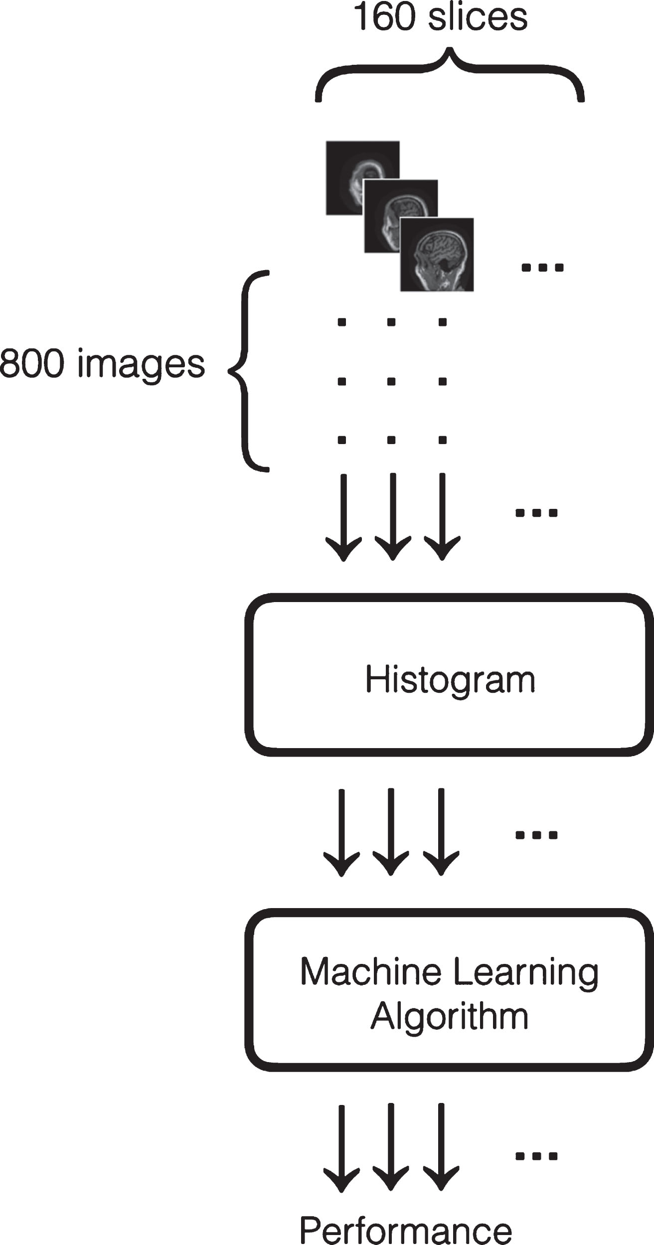
Flowchart of histogram-based classification.

Supervised learning algorithms

Multiple machine learning algorithms were being used in this study. SVM methods have been extensively used in many studies and yield promising results. Also, other supervised learning algorithms used in this study include decision trees, logistic regression, SVM, K-Nearest Neighbor, and Ensemble.

Decision trees

Decision tree is a popular classification algorithm that uses a tree-like structure to predict the category of a new data point. The features of the database are known as attributes and the tree itself is built on nodes and branches. At each node, a certain attribute is examined and based on the result, it splits into two branches. The process is continued until a label is given and at that stage, the branch is called a leaf [27].

Logistic regression

Logistic regression is a commonly used technique in binary classification problems. It usually makes use of the sigmoid function. This function can map the values of the used features into a probability value ranging between 0 and 1. Classification is done using a certain threshold to label the data point as one of two classes.

Support vector machine

SVM is an algorithm in machine learning used to solve classification and regression problems. SVM is more commonly used in classification challenges in supervised learning by classifying data with similar features and separating those which are different. As described by Cortes and Vapnik, SVM works by finding a hyperplane in a number of dimensions that corresponds to the number of features in a database [28]. Defining this hyperplane is concluded so that it specifies the boundaries to give us more certainty in the decision of classifying additional points in the database. Classification in SVM is based on linear separation which might not yield good results and in such cases SVM performance can be improved by projecting on nonlinear function (kernel) [29]. The error is being minimized in SVM algorithm by maximizing the margin between the features and the hyperplane separating the two classes [29].

K-Nearest Neighbor (KNN)

Nearest Neighbor method is a machine learning algorithm in which data is classified based on the class of its neighbors [30, 31]. For one data point that has no class, a sphere is drawn around it with k points included; the point is assigned the class with the largest class present in the other points inside the sphere. In KNN algorithm, the labels must be included in the data. Cover and Hart present detailed explanation of the algorithm [30].

Ensemble

Ensemble algorithm is a machine learning algorithm that uses multiple classifiers to make predictions on the data by combining the outcome of those classifiers [32]. Some of the main algorithms used in the ensemble method are bagging, boosting, AdaBoost, and stacked generalization [33]. Bagging predictors divide the database into sets of training data and train the same classifier on those sets; the prediction of each classifier is combined in which the final prediction is based on majority voting [33]. Similar to bagging, boosting algorithm divides the training data into sets and make final predictions using majority voting. In boosting method, majority voting is done on several weak classifiers in which it combines the predictions of those weak classifier to result in a strong classifier. AdaBoost method works by training a weak classifier on subsets of the training data in which the weight of the classifier is included in the hypowork [33]. The output is the weighted vote of the predicted classes from the combined weak classifiers. Additional information on ensemble techniques are found in [33].

Majority vote

Majority vote is a process of combining all classifiers and making predictions based on the majority result of all the classifiers. It is a simple way of combining multiple classifiers outputs [34 –36]. In case of this research work, there is two classes; predictions of each algorithm is tested based on trained model. All the results are combined and a final prediction from the combined model is generated based on the majority of all the predictions using majority vote. For example, the class is 1 if more than half the predictions of the algorithms are 1 and 0 if more than half the predictions are 0. In this work, 22 classifiers were used in which the majority vote was done based on having more than 11 of the same class.

Weighted vote

Weighted vote was also applied in this research work by assigning a certain weight for each algorithm based on the accuracy of the trained model. The weights were used as counts for the labels for every test data point. The final prediction is based on the label that has the maximum counts. In this part, 22 classifiers were used.

RESULTS AND DISCUSSION

In this section, the results shown are done using 800 images with 400 AD and 400 CN, where the 3-dimensional images were represented in sagittal plane. Table 2 shows part of the results for the run of 800 subjects for 160 slices; the number of features used is 256 which are the number of bins used in getting the histogram of the images. Performance accuracy of all 160 slices was being studied, in which fine tree, logistic regression, linear SVM, quadratic SVM, cubic SVM, fine Gaussian SVM, medium Gaussian SVM, coarse Gaussian SVM, fine KNN, medium KNN, and ensemble boosted trees were being compared in regard to accuracy.

Table 2

Performance for slices 31–40. Methods used 800 images (400 AD and 400 CN)

	Slice accuracy (%)
Method	31	32	33	34	35	36	37	38	39	40
Fine Tree	58.2	56.0	54.0	54.4	55.0	51.2	52.4	54.4	53.8	51.7
Logistic Regression	48.8	48.8	46.6	50.1	52.4	54.1	51.7	52.1	49.5	52.4
Linear SVM	54.1	57.0	53.6	56.9	59.1	61.1	57.9	59.0	57.1	57.8
Quadratic SVM	59.8	60.9	55.6	60.5	58.6	61.8	62.0	57.8	60.0	59.2
Cubic SVM	58.6	57.5	58.8	61.0	59.0	63.5	62.1	58.9	57.8	59.9
Fine Gaussian SVM	54.0	55.0	55.0	56.1	55.1	52.5	56.1	57.2	56.0	52.2
Median Gaussian SVM	59.2	60.9	59.6	61.3	61.6	62.3	64.0	61.4	62.3	61.3
Coarse Gaussian SVM	54.8	56.8	56.4	56.2	57.6	58.9	58.0	57.0	56.6	56.0
Fine KNN	57.2	56.6	57.2	57.9	58.1	59.1	61.4	57.5	58.4	57.0
Medium KNN	57.1	57.6	58.0	55.5	57.8	62.1	58.6	59.2	59.8	55.6
Ensemble Boosted Trees	60.0	61.5	57.1	58.1	61.5	58.6	58.8	58.0	57.4	56.8

Table 2 shows comparison of slices between 31 and 40 in which bold values are the highest accuracy for each classifier in regard to the whole row from slice 1 to 160 in which slices 36 and 37 shows the highest accuracy in 6 classifiers.

In Fig. 4, the maximum accuracy for 160 slices for 800 subjects (400 AD and 400 CN) is plotted for multiple classifiers mentioned earlier in this document. Figure 4 show that the accuracy for the slices in the beginning and toward the end have lower accuracy in the classification between AD versus CN, implying that these slices are not a good examination for the classification problem giving into account that in those slices the brain has not been shown yet and then gradually appears. In Figs. 5 and 6, an example is shown for slice numbers 5, 10, and 15 for one of the subjects which shows no sign of the brain in the images yet which explains why the accuracy is very low for the classification problem in the early slices; the case is the same for the slices toward the end.

Fig.4

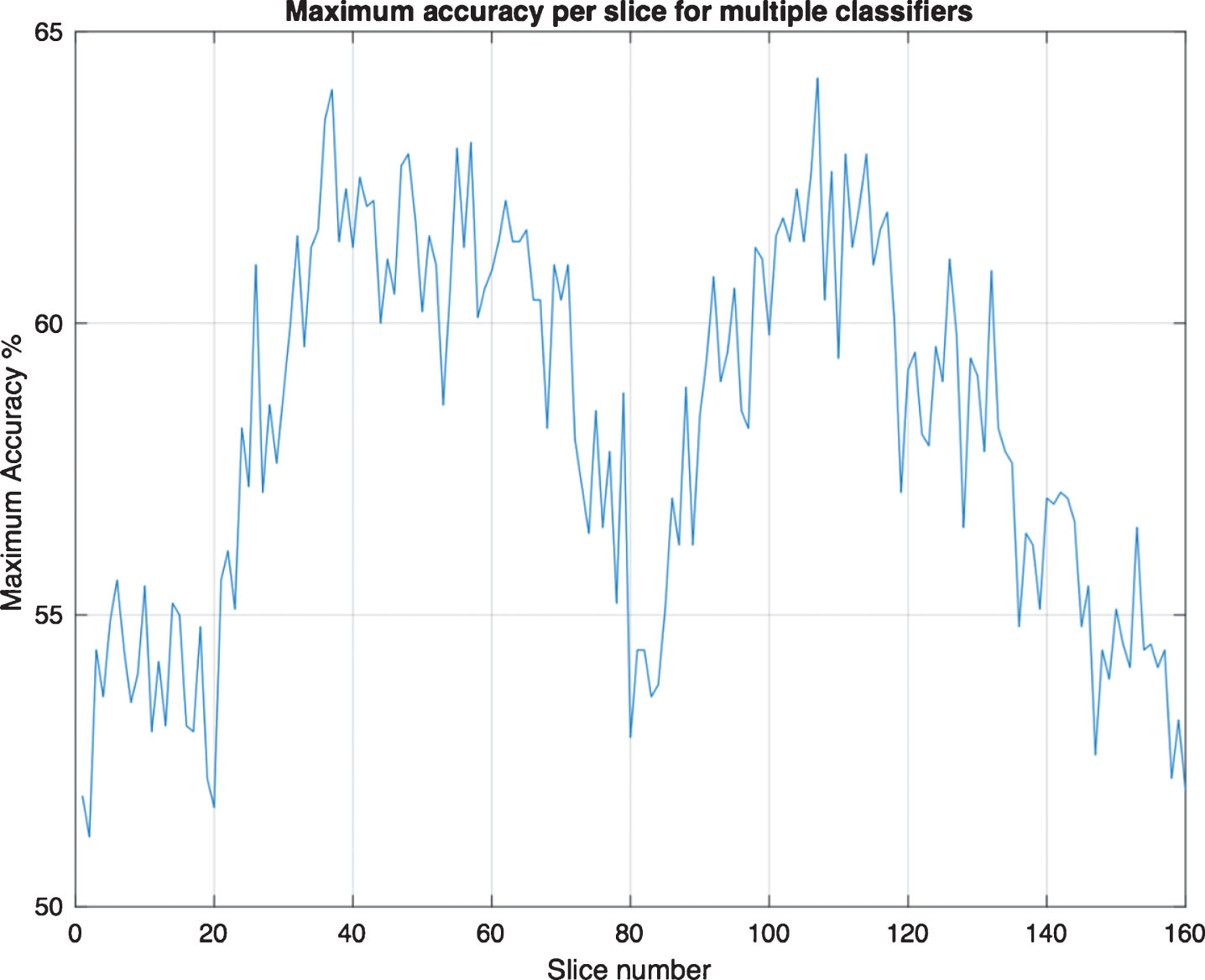
Maximum accuracy per slice for multiple classifiers.

Fig.5

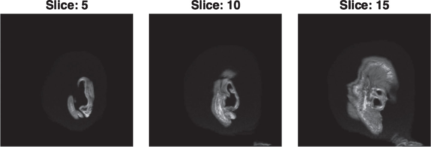
AD image slices 5, 10, and 15.

Fig.6

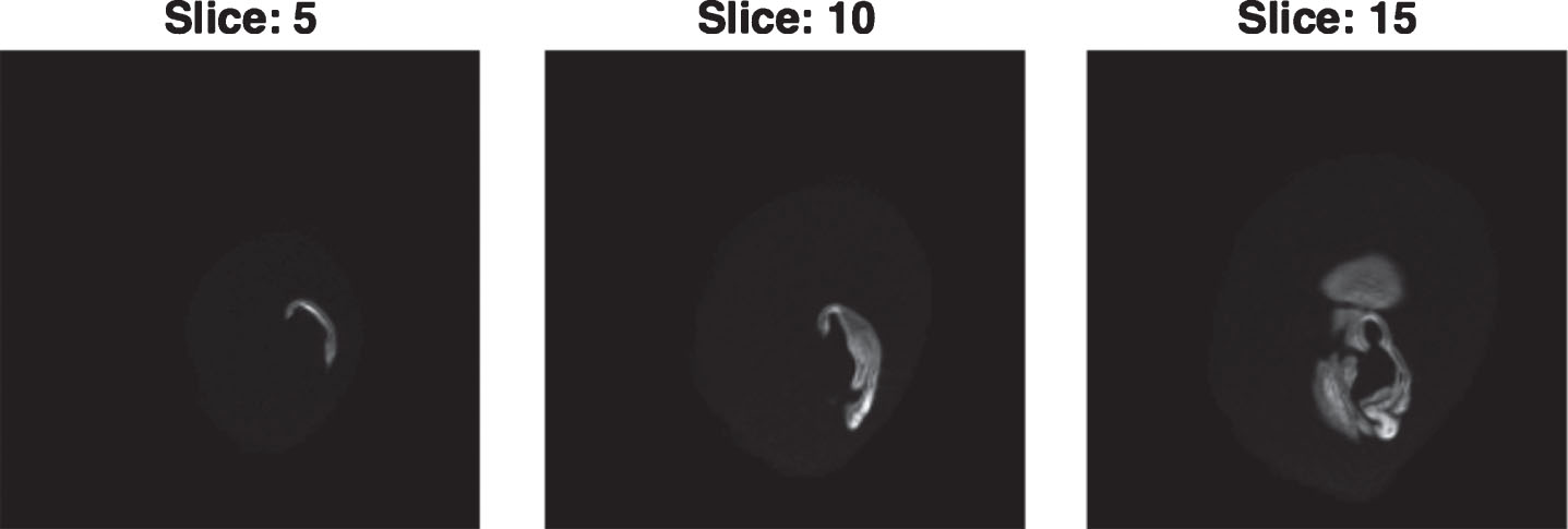
CN image slices 5, 10, & 15.

In Fig. 7, the maximum and minimum accuracy for 160 slices for 800 subjects (400 AD and 400 CN) is plotted for multiple classifiers mentioned earlier in this document.

Fig.7

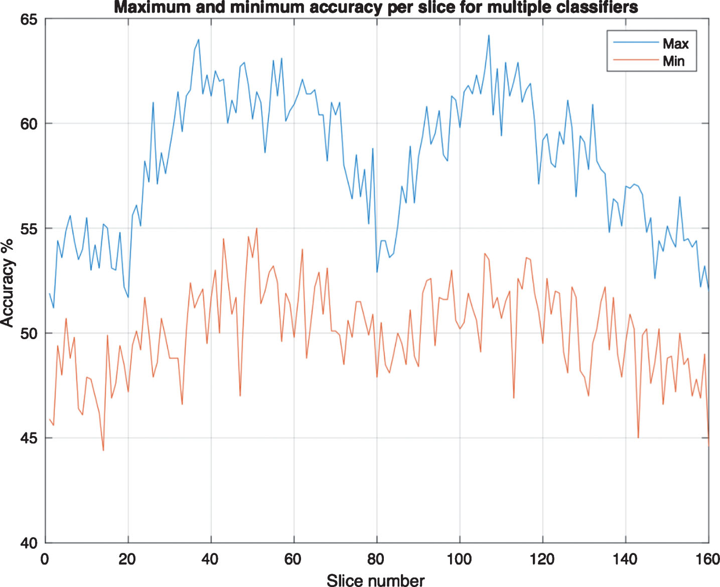
Maximum and minimum accuracy per slice for multiple classifiers.

Table 2 shows comparison of slices between 31 and 40. It can be shown from this table that medium Gaussian SVM performed highest with most of the slices. Figure 8 shows the accuracy of fine tree, medium Gaussian SVM, and medium KNN for the 160 slices. As shown in the figure, medium Gaussian SVM has the highest accuracy in most points.

Fig.8

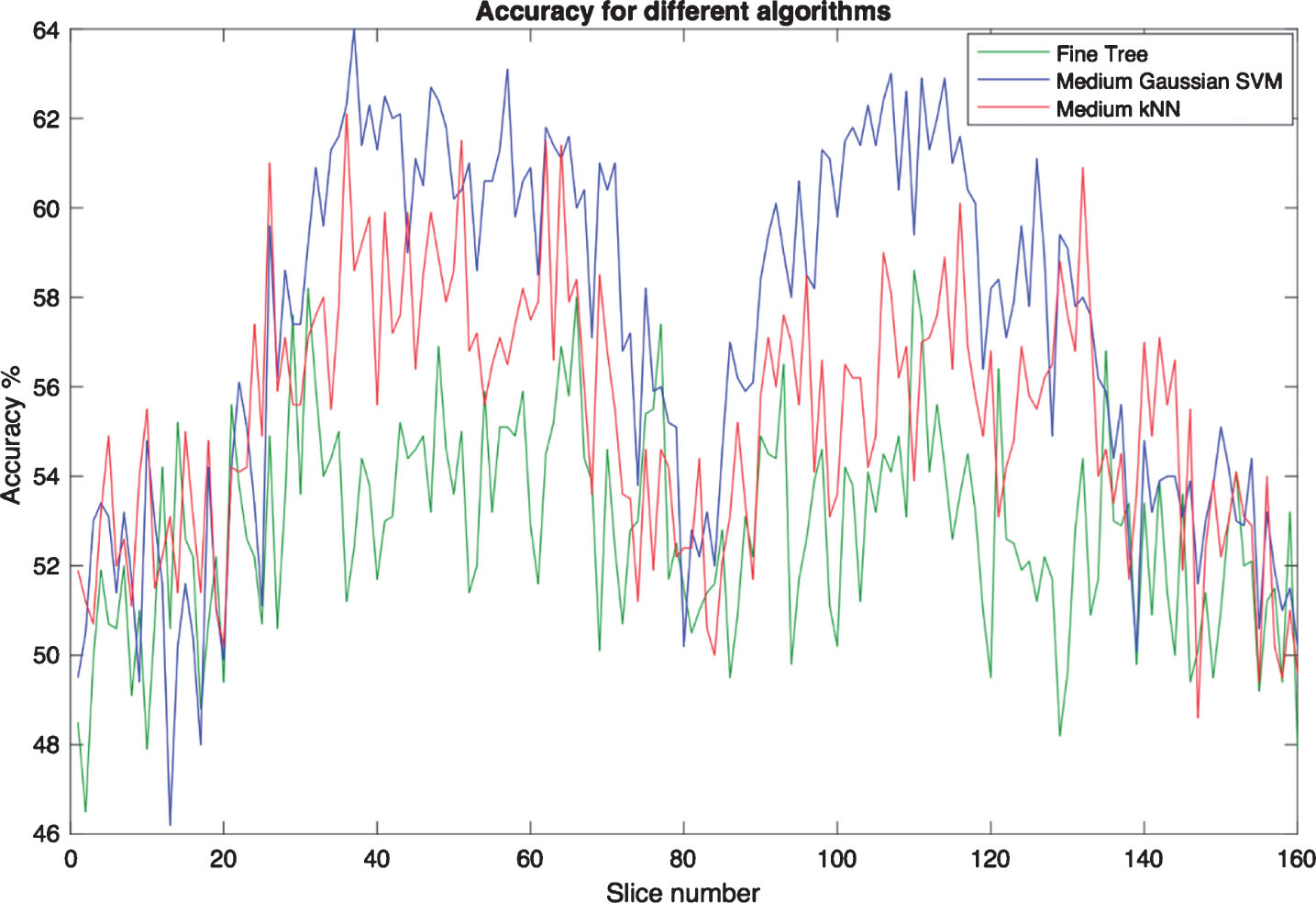
Comparison between Fine Tree, Medium Gaussian SVM, and Medium KNN accuracy.

Slices 36 and 37 are considered for further inspection, since as shown earlier in Table 2, the accuracy is highest in those two slices in the classification between AD and CN. Therefore, medium Gaussian SVM for the trained model for slices 36 and 37 was used for testing all other slices giving the results in Table 3.

Table 3

Performance for testing data for slices 31–40 using trained model of slice 36 and 37

	Slice Accuracy (%)
	31	32	33	34	35	36	37	38	39	40
Median Gaussian SVM trained on slice 36	60.50	62.13	65.50	68.38	70.75		69.25	69.00	67.75	65.75
Median Gaussian SVM trained on slice 37	58.13	61.63	63.25	65.13	67.50	70.88		69.75	68.75	68.13

Table 3 show the highest accuracy highlighted for the trained model for slice 36 and 37, which is used to test all other 160 slices. After testing the data for other slices using trained model of slice 36 using medium Gaussian SVM classifier, an accuracy of 70.75% for slice number 35 achieves highest accuracy. Respectively, for trained model of slice 37, an accuracy of 70.87% was achieved for slice 36 as testing data.

As slice 35 and slice 36 showed the highest performance from trained model of slice 36 and 37, respectively, for medium Gaussian SVM, majority voting and weighted voting were applied including 22 classifiers. A model was trained using slice 36 as training data in which predictions were made from slice 35 as test data. Majority voting was applied from the prediction of 22 classifiers in which results show an accuracy of 74.12% and an accuracy of 74.75% for weighted voting. Another model was trained using slice 37 as training data and slice 36 as test data in which an accuracy of 74.62% was obtained for majority voting and 75.87% for weighted voting. A comparison of the results for majority vote and weighted vote for slice 35 and 36 as test data is shown in Fig. 9.

Fig.9

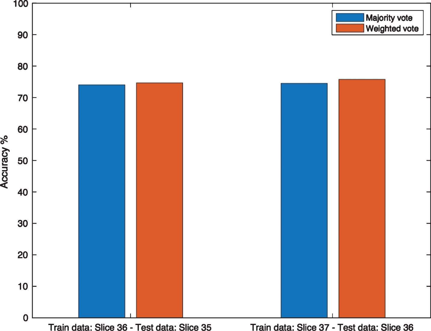
Accuracy for majority and weighted vote for trained model on slice 36 and 37.

Figure 10 show slices 36, 37, and 38 that are taken for further investigation as training data showed the highest accuracy in the classification between AD and CN in those slices.

Fig.10

AD and CN image slices 36, 37, and 38.

Histograms of slice 36 and 37 for all the 800 images were concatenated in one matrix of 800 rows and 512 columns (corresponding to number of features). The database was divided into 600 images as training data and 200 images as testing data both divided equally into AD and CN. All classifiers were trained with all the 512 features. The corresponding model for each classifier was saved and tested against the test data. A matrix of all predictions for the test data using all trained models was formed. Majority voting was applied for all the predictions, and the results were compared to actual data labels. The accuracy of the majority vote for slice 36 and 37 is 69.5%. The same procedure was done for concatenating slices 36, 37, and 38. For slices 36, 37, and 38, the number of features is 768 and the accuracy of majority vote is in this case 64.5%. Weighted voting was also applied for all the predictions based on the accuracy of the trained model and the results were compared to actual data labels. The accuracy of the weighted vote for slice 36 and 37 is 67.5%. For slices 36, 37, and 38, the accuracy of weighted vote is 63.5%. Figure 11 shows a comparison of the results for majority vote and weighted vote for concatenation of slices 36 and 37 and slices 36, 37, and 38.

Fig.11

Accuracy for majority and weighted vote.

Conclusion

In this research, different machine learning algorithms were tested for classification of AD and CN. Images of MRI brain scans were obtained from the ADNI database in the format of NIfTI files. The main experiment of this research work is classification of slices using histogram for data representation. Accuracy for different slices were investigated in which certain slices showed the most promising results. Slices 36 and 37 were selected based on accuracy results for further examination. Histogram of slices resulted in accuracy of 69.5% for classification by concatenating histogram of slices 36 and 37 as well as slices 36, 37, and 38 and using majority voting technique. The data was divided into training data and testing data. The same procedure was done to calculate the weighted vote and compare it to the actual labels. The weighted vote for slice 36 and 37 resulted in accuracy of 67.5%.

Footnotes

ACKNOWLEDGMENTS

This work has been partially supported by the Estonian Centre of Excellence in IT (EXCITE) funded by the European Regional Development Fund.

Authors’ disclosures available online ().

References

Castellani

, Perry

, Iverson

(2015) Chronic effects of mild neurotrauma: Putting the cart before the horse? J Neuropathol Exp Neurol 74, 493–499.

Castellani

, Perry

(2014) The complexities of the pathology–pathogenesis relationship in Alzheimer disease. Biochem Pharmacol 88, 671–676.

Zhang

, Wang

, Phillips

, Yang

, Yuan

(2016) Three-dimensional eigenbrain for the detection of subjects and brain regions related with Alzheimer’s disease. J Alzheimers Dis 50, 1163–1179.

Alzheimer’s Disease & Dementia. Alzheimer’s Association, http://www.alz.org/alzheimers_disease_what_is_alzheimers.asp, Last updated 2019, Accessed on February 14, 2019.

Zhang

, Wang

, Sui

, Yang

, Liu

, Cheng

, Sun

, Jia

, Philips

, Gorriz

(2018) Multivariate approach for Alzheimer’s disease detection using stationary wavelet entropy and predator-prey particle swarm optimization. J Alzheimers Dis 65, 855–869.

Brookmeyer

, Johnson

, Ziegler-Graham

, Arrighi

(2007) Forecasting the global burden of Alzheimer’s disease. Alzheimers Dement 3, 186–191.

Alzheimer’s Disease and Dementia. Alzheimer’s Association, https://www.alz.org/alzheimers-dementia/what-is-dementia, Last updated 2019, Accessed on February 14, 2019.

Alzheimer’s Disease and Dementia. Alzheimer’s Association, https://www.alz.org/alzheimer_s_dementia, Last updated 2019, Accessed on April 18, 2019.

Prince

, Bryce

, Ferri

(2011) World Alzheimer Report 2011: The benefits of early diagnosis and intervention. Alzheimer’s Disease International, London, UK.

10.

Alzheimer’s Disease and Dementia. Alzheimer’s Association, https://www.alz.org/alzheimers-dementia/research_progress/earlier-diagnosis, Last updated 2019, Accessed on April 20, 2019.

11.

Zhang

, Shen

, Alzheimer’s Disease Neuroimaging Initiative (2012) Multi-modal multi-task learning for joint prediction of multiple regression and classification variables in Alzheimer’s disease. Neuroimage 59, 895–907.

12.

Westman

, Muehlboeck

, Simmons

(2012) Combining MRI and CSF measures for classification of Alzheimer’s disease and prediction of mild cognitive impairment conversion. Neuroimage 62, 229–238.

13.

Zhou

, Goryawala

, Cabrerizo

, Wang

, Barker

, Loewenstein

, Duara

, Adjouadi

(2014) An optimal decisional space for the classification of Alzheimer’s disease and mild cognitive impairment. IEEE Trans Biomed Eng 61, 2245–2253.

14.

Gray

, Aljabar

, Heckemann

, Hammers

, Rueckert

, Alzheimer’s Disease Neuroimaging Initiative (2013) Random forest-based similarity measures for multi-modal classification of Alzheimer’s disease. Neuroimage 65, 167–175.

15.

Papakostas

, Savio

, Graña

, Kaburlasos

(2015) A lattice computing approach to Alzheimer’s disease computer assisted diagnosis based on MRI data. Neurocomputing 150, 37–42.

16.

Zhang

, Wang

, Zhou

, Yuan

, Shen

, Alzheimer’s Disease Neuroimaging Initiative (2011) Multimodal classification of Alzheimer’s disease and mild cognitive impairment. Neuroimage 55, 856–867.

17.

Mahmood

, Ghimire

(2013) Automatic detection and classification of Alzheimer’s Disease from MRI scans using principal component analysis and artificial neural networks. In 2013 20th International Conference on Systems, Signals and Image Processing (IWSSIP), IEEE, pp. 133–137.

18.

Ding

, Zhang

, Lan

, Qin

, Zhang

, Wang

(2015) Classification of Alzheimer’s disease based on the combination of morphometric feature and texture feature. In 2015 IEEE International Conference on Bioinformatics and Biomedicine (BIBM), IEEE, pp. 409–412.

19.

Alzheimer’s Disease Neuroimaging Initiative. About ADNI, http://adni.loni.usc.edu/about/, Last updated 2019, Accessed on May 2, 2019.

20.

Alzheimer’s Disease Neuroimaging Initiative. Background & Rationale, http://adni.loni.usc.edu/study-design/, Last updated 2019, Accessed on May 2, 2019.

21.

Alzheimer’s Disease Neuroimaging Initiative. MRI Pre-processing, http://adni.loni.usc.edu/methods/mri-tool/mri-analysis/#mri-pre-processing-container, Last updated 2019, Accessed on May 2, 2019.

22.

Alzheimer’s Disease Neuroimaging Initiative. MRI Pre-processing, http://adni.loni.usc.edu/study-design/#study-objective-container, Last updated 2019, Accessed on May 2, 2019.

23.

Gonzalez

, Woods

(2002) Digital Image Processing Second Edition. Prentice-Hall, Inc., Upper Saddle River, NJ.

24.

Anbarjafari

(2015) An objective no-reference measure of illumination assessment. Measure Sci Rev 15, 319–322.

25.

Beheshti

, Maikusa

, Matsuda

, Demirel

, Anbarjafari

(2017) Histogram-based feature extraction from individual gray matter similarity-matrix for Alzheimer’s disease classification. J Alzheimers Dis 55, 1571–1582.

26.

Beheshti

, Maikusa

, Daneshmand

, Matsuda

, Demirel

, Anbarjafari

(2017) Classification of Alzheimer’s disease and prediction of mild cognitive impairment conversion using histogram-based analysis of patient-specific anatomical brain connectivity networks. J Alzheimers Dis 60, 295–304.

27.

Kingsford

, Salzberg

(2008) What are decision trees? Nat Biotechnol 26, 1011.

28.

Cortes

, Vapnik

(1995) Support-vector networks. Mach Learn 20, 273–297.

29.

Amari

, Wu

(1999) Improving support vector machine classifiers by modifying kernel functions. Neural Netw 12, 783–789.

30.

Cover

, Hart

(1967) Nearest neighbor pattern classification. IEEE Trans Inf Theory 13, 21–27.

31.

Steenwijk

, Pouwels

, Daams

, van Dalen

, Caan

, Richard

, Barkhof

, Vrenken

(2013) Accurate white matter lesion segmentation by k nearest neighbor classification with tissue type priors (kNN-TTPs). Neuroimage Clin 3, 462–469.

32.

Dietterich

(2000) Ensemble methods in machine learning. In International Workshop on Multiple Classifier Systems, Springer, Berlin, Heidelberg, pp. 1–15.

33.

Polikar

(2006) Ensemble based systems in decision making. IEEE Circuits Systems Magazine 6, 21–45.

34.

Lam

, Suen

(1994) A theoretical analysis of the application of majority voting to pattern recognition. In Proceedings of the 12th IAPR International Conference on Pattern Recognition, Vol. 3-Conference C: Signal Processing (Cat. No. 94CH3440-5), Vol. 2. IEEE, pp. 418–420.

35.

Hsu

(2017) A theoretical analysis of why hybrid ensembles work. Comput Intell Neurosci 2017, 1930702.

36.

Mohandes

, Deriche

, Aliyu

(2018) Classifiers combination techniques: A comprehensive review. IEEE Access 6, 19626–19639.