Integrating Convolutional Neural Networks and Multi-Task Dictionary Learning for Cognitive Decline Prediction with Longitudinal Images

Abstract

Background:

Disease progression prediction based on neuroimaging biomarkers is vital in Alzheimer’s disease (AD) research. Convolutional neural networks (CNN) have been proved to be powerful for various computer vision research by refining reliable and high-level feature maps from image patches.

Objective:

A key challenge in applying CNN to neuroimaging research is the limited labeled samples with high dimensional features. Another challenge is how to improve the prediction accuracy by joint analysis of multiple data sources (i.e., multiple time points or multiple biomarkers). To address these two challenges, we propose a novel multi-task learning framework based on CNN.

Methods:

First, we pre-trained CNN on the ImageNet dataset and transferred the knowledge from the pre-trained model to neuroimaging representation. We used this deep model as feature extractor to generate high-level feature maps of different tasks. Then a novel unsupervised learning method, termed Multi-task Stochastic Coordinate Coding (MSCC), was proposed for learning sparse features of multi-task feature maps by using shared and individual dictionaries. Finally, Lasso regression was performed on these multi-task sparse features to predict AD progression measured by the Mini-Mental State Examination (MMSE) and the Alzheimer’s Disease Assessment Scale cognitive subscale (ADAS-Cog).

Results:

We applied this novel CNN-MSCC system on the Alzheimer’s Disease Neuroimaging Initiative dataset to predict future MMSE/ADAS-Cog scales. We found our method achieved superior performances compared with seven other methods.

Conclusion:

Our work may add new insights into data augmentation and multi-task deep model research and facilitate the adoption of deep models in neuroimaging research.

Keywords

Alzheimer’s disease convolutional neural networks dictionary learning multi-task learning transfer learning

INTRODUCTION

Alzheimer’s disease (AD) is the most prevalent neurodegenerative brain disease worldwide [1, 2]. Clinical trial failures in symptomatic patients have led to the belief that capturing brain changes and therapeutically intervening at earlier disease stages would be more likely to achieve disease modification [3]. Various modalities of biomarkers have been used for early identification of brain changes related to AD and its earlier symptomatic stage, mild cognitive impairment (MCI), including the brain structural atrophy measured by magnetic resonance imaging (MRI) [4 –6], metabolic alterations in the brain measured by fluorodeoxyglucose positron emission tomography (FDG-PET) [7, 8], and pathological amyloid depositions measured through cerebrospinal fluid (CSF) and amyloid-PET [3, 9]. Of these, abnormal structural MRI is considered as a typical marker of neurodegeneration and retains a close relationship with cognitive performance through the clinical phases of MCI and dementia [3]. MRI is more widely available, less invasive, and more affordable for clinical applications than other imaging biomarker modalities. To date, the inevitable deformations of hippocampus, ventricle, and cortical thickness are well captured by structural MRI (Fig. 1) [10 –13]. Prior work [3 , 14–16], including our own study in a cognitively unimpaired brain imaging cohort (Arizona APOE cohort) [10], indicated that MRI hippocampal atrophy accelerates 20 + years prior to incident to MCI. Thus, structural MRI is promising as a potential preclinical AD biomarker. However, MRI biometrics do not yet reliably predict diagnosis and prognosis in early AD stages especially in individual patients [2, 17–20 , 2, 17–20].

Fig. 1

Three promising brain structure measures of the structural MR images used for clinical diagnosis of Alzheimer’s disease: (a) Hippocampal contractions; (b) Ventricle expansions; (c) Cortical thickness reductions.

Convolutional neural networks (CNN) are capable of learning comprehensive feature maps from images [21]. CNN has been successfully applied to a variety of computer vision and medical imaging applications including image classification [22], segmentation [23], and disease diagnosis [24]. It has the potential to improve the predictability of AD progression [21]. Li et al. [25] proposed a CNN framework for early prognosis of AD dementia based on the baseline hippocampal MRI data, and demonstrated improved performance for predicting progression to AD dementia. However, there are still few CNN studies on modeling AD progression. One issue is the limited training data in the AD research domain while transfer learning has been proven to be a highly effective technique for limited medical image analysis. Kermany et al. [26] successfully applied CNN with transfer learning to classify images for macular degeneration and diabetic retinopathy and distinguish bacterial and viral pneumonia on chest X-rays. Xu et al. [27] designed a deep model of CNN with transfer learning and achieved a good performance in distinguishing histopathology images of low and high tumor mutational burden patients. CNN with transfer learning, therefore, has potential for AD dementia diagnostic modeling based on MR images.

After using CNNs with transfer learning, we confront an additional challenge that is high dimensional feature maps derived from small number of individual biomarkers based on MR images. To address this so called “large p, small n” problem, sparse coding has been applied. Sparse coding is an effective way of learning a small number of basis vectors termed dictionary to represent high dimensional features effectively and concisely [28 –30]. However traditional dictionary learning algorithms confront challenges of handling very large training sets or dynamic training data changing over time, such as MR image sequences accompanying AD progression [30]. Studies of [17 , 31–33] demonstrated that joint analysis of multi-tasks (i.e., multiple time points or biomarkers) improved the prediction performance and may be used for tracking AD progression.

To track AD progression measured by cognitive scores, Zhang and Shen [18] proposed Multi-Modal Multi-Task learning to jointly predict multiple variables from multi-modal data. However, they excluded conditions of missing values in both modalities and tasks. The study of [17] proposed Multi-Task Learning formulations by considering the prediction at each time point as a task. It demonstrated that Multi-Task Learning outperformed single-task learning algorithms including ridge regression and Lasso for AD progression. However, their approaches treated dictionary learning for all tasks in the same manner, which was suboptimal for modeling AD progression. To address the above two issues, our previous study [32] proposed a two-stage Multi-task Stochastic Coordinate Coding (MSCC), stage 1 involved multi-source dictionary learning to utilize the common and individual sparse features in multi-tasks. In stage 2, a Multi-Task Learning method was developed to solve the missing values issue. Experimental results demonstrated that MSCC had an improved prediction accuracy and speed efficiency for future AD clinical score predictions compared to other similar algorithms.

To explore the statistical power of the combination of CNN with transfer learning and multi-task sparse coding, we developed an advanced deep model CNN-MSCC to predict AD progression measured by the Mini-Mental State Examination (MMSE) [34] and the Alzheimer’s Disease Assessment Scale cognitive subscale (ADAS-Cog) [35] scores using multi-task imaging biomarkers. We hypothesized that our system may produce accurate AD progression modeling results while offering the flexibility to work with structural imaging features from both longitudinal data and multiple regions-of-interest (ROIs). To validate our hypothesis, we designed two sets of experiments where we applied our framework to study the structural MRI data from Alzheimer Disease Neuroimaging Initiative (ADNI) [36, 37] and compared our approach with seven other similar methods. In Experimental I, we aimed to use longitudinal (baseline, 6-months, 12-months) hippocampal structural measures to predict MMSE/ADAS-Cog scales of 24-months subjects. In Experiment II, we applied the proposed framework on three kinds of baseline structural features (hippocampal morphometry, lateral ventricular morphometry, and cortical thickness) to predict MMSE/ADAS-Cog scales of varied time points (6-months, 12-months, and 24-months).

MATERIALS AND METHODS

Subjects

Data for testing the performances of our proposed framework and comparison methods were obtained from the ADNI database (http://adni.loni.usc.edu). The ADNI was launched in 2003 as a public-private partnership, led by Principal Investigator Michael W. Weiner, MD. The primary goal of ADNI is to test whether biological markers such as serial MRI and positron emission tomography (PET), combined with clinical and neuropsychological assessment can measure the progression of MCI and early AD. The structural MR images were acquired from 1.5T scanners. The raw MR images and MMSE/ADAS-Cog scales were downloaded from the public ADNI website (http://adni.loni.usc.edu/).

In this work, all of these performance comparison analysis have been conducted on ADNI-I dataset which including 837 subjects, the selection criteria can refer our previous study [38], the identification numbers of subjects were included in Supplementary Material A. There were 837 baseline subjects between 68–82 years of age, 733 subjects in the 6th months, and 676 subjects in the 12th months, and 544 subjects in the 24th months. There were 814 baseline subjects having MMSE/ADAS-Cog scores, including 1) 186 AD subjects: baseline MMSE scores between 20–26, 2) 399 MCI subjects: baseline MMSE scores between 24–30, and 3) 229 cognitive unimpaired (CU) subjects: baseline MMSE scores between 24–30. The demographics of subjects used in our experiments are shown in Table 1.

Table 1

Demographic characteristics and longitudinal neuropsychological scores of the subjects

Baseline sample size of each group	AD (n = 186)	CU (n = 229)	MCI (n = 399)
Male/Female	98/88	119/110	255/144
Age	75.36±7.57	75.97±5.04	74.85±7.37
Education	14.69±3.12	15.96±3.05	15.54±3.24
MMSE (Baseline)	23.28±2.05	29.09±1.05	27.01±1.79
MMSE (6-months)	20.88±6.50	27.96±5.47	25.06±6.40
MMSE (12-months)	17.69±8.78	26.72±8.13	23.69±8.40
MMSE (24-months)	13.36±9.87	25.67±9.46	19.16±11.40
ADAS-Cog (Baseline)	29.03±7.66	9.55±4.34	18.71±6.28
ADAS-Cog (6-months)	28.05±12.70	9.21±5.04	18.63±8.89
ADAS-Cog (12-months)	27.34±16.46	7.83±5.13	18.15±10.08
ADAS-Cog (24-months)	24.79±21.15	8.20±5.63	16.75±13.09

AD, Alzheimer’s disease; CU, cognitive unimpaired; MCI, mild cognitive impairment; MMSE, Mini-Mental State Examination; ADAS-Cog, Alzheimer’s Disease Assessment Scale-Cognitive Subscale.

Proposed pipeline

In this section, we introduce the CNN-MSCC framework which predicts future MMSE/ADAS-Cog based on previous image patches from multiple time points or multiple ROIs. We pre-trained the CNN model on the ImageNet dataset [22, 39]. Surface measures of hippocampi, lateral ventricle, and cortical thickness were estimated from individual structural MR images [6, 40]. Surface maps were first constructed for these ROIs, and image patches were further extracted from these surface maps [29 , 42]. With the transfer learning strategy, the pre-trained CNN network was adopted as a feature extractor for the following multi-task learning process (i.e., different time points or ROIs) [31]. We further employed MSCC to conduct the multi-task learning to simultaneously refine sparse features and dictionaries [32]. Finally, we employed the sparse codes generated from MSCC to perform the Lasso and predict the future MMSE/ADAS-Cog scores [43]. The entire pipeline of our proposed framework is illustrated in Fig. 2.

Fig. 2

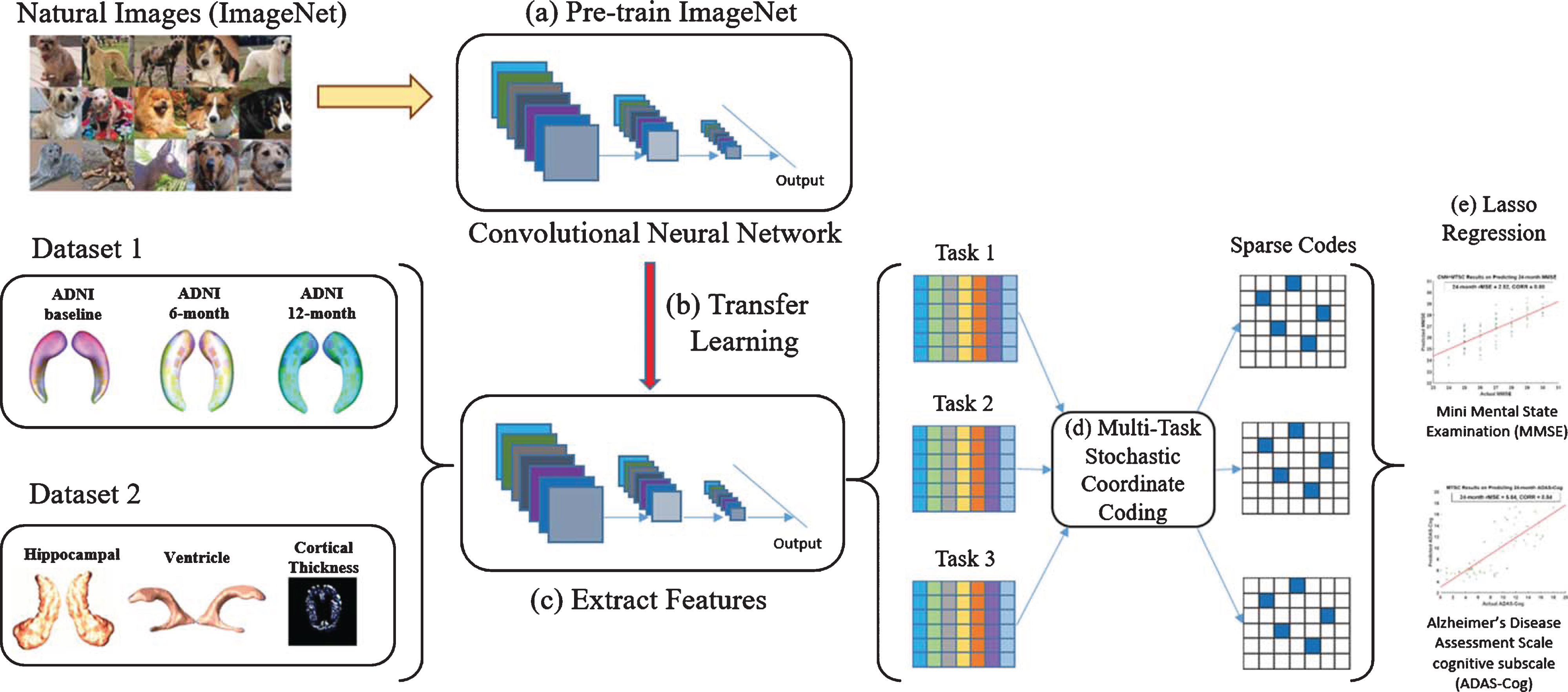
An illustration of the proposed CNN-MSCC framework. The CNN model was pre-trained on the ImageNet dataset (a). The pre-trained model was modified as a feature extractor for brain structural MR image patches based on transfer learning strategy (b) and deep feature maps were extracted from varied structural measures or time slots (c). MSCC was adopted to generate the sparse features from deep feature maps (d). Finally, Lasso regression was applied on the sparse features to predict future MMSE and ADAS-Cog scores (e).

MR image preprocessing

Hippocampal surfaces were firstly segmented and reconstructed from individual MR images using FIRST software [44] and marching cube method [45]. Then, we computed hippocampal conformal grids on the Euclidean domain with holomorphic 1-form functions [46]. With these conformal grids, we transferred the original 3D hippocampal structure into 2D vertex-based features. The benefit of the conformal parameterization is that it helped compute both surface intrinsic and extrinsic geometry features, and dramatically simplified the implementation of surface fluid registration algorithm [47]. We further applied the inverse consistent surface fluid registration method to register hippocampal surfaces across subjects. After the surface registration, we introduced consistent image-grid like mesh structures on all hippocampal surfaces, for each subject, a 90,000-dimensional mesh structure represented mTBM of the hippocampal (HP) surfaces. To reduce the high mesh dimension, we can treat the surface-based feature structure as the pixel-grid and build patch structures. Quadrilateral patches were adopted here to improve the computational efficiency. Specifically, with the rectangular surface parameterization obtained in our surface fluid registration [47], taking advantage of the regular grid-like mesh structure, we randomly generated a number of square windows (50 × 50 vertices) on each registered surface to obtain a collection of small surface patches with different amounts of overlaps. We choose 132 patches on each hippocampus because it will cover all the vertices on each side of hippocampus. The procedure is in fact equivalent to applying a low-pass filter on the original meshes. As a result, the geometrical structures are still present while surface feature variances are reduced. We performed the same procedure to compute patches on both lateral ventricular and cortical surfaces. Finally, we represent the original bilateral hippocampal surface features with 264 overlapping patches [29]. It is worth noting that even though we randomly select patches on all subjects, because of the registered surfaces, the patches we select in each task are in fixed locations on each hippocampus. Figure 3 shows an example of patch selection on a pair of the hippocampal surfaces. As these patches are allowed to overlap, a vertex may be contained in several patches. The zoom-in windows in Fig. 3 show overlapping areas of selected patches. In this way, we can still keep the surface spatial structure and learn the mesh structures.

Fig. 3

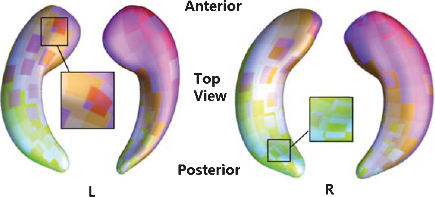
Visualization of selected surface patches on a pair of the hippocampal surfaces. In this figure, we show some randomly selected surface patches with different amounts of overlapping. The zoom-in pictures show some overlapping areas between surface patches. We generate a series of square windows on each side of hippocampus.

Further, we created surface mesh models of the lateral ventricles using our multi-atlas fluid image alignment (MAFIA) method that combines multiple fluid registrations to boost accuracy [48]. To model the lateral ventricular surfaces, we automatically located and introduced three cuts, based on the topology of the lateral ventricles, in which several horns are joined together at the ventricular “atrium” or “trigone” [6]. With the holomorphic flow segmentation method, each lateral ventricular surface was automatically partitioned into three pieces [46]. These three pieces are roughly three horns of the lateral ventricle: anterior horn, posterior horn, and inferior horn. The surface segmentation was done by tracing curves that went through the zero point and had equal parameter coordinates. Then we registered each segmented surface of the lateral ventricular surfaces across subjects using constrained harmonic maps and computed mTBM features. For each subject, a 308,247-dimensional mTBM statistics were computed from registered ventricular surfaces. We randomly generated a number of square windows (50×50) on each registered surface to obtain a collection of small surface patches with different amounts of overlaps, 1,713 image patches on each ventricular surface were chosen.

We adopted FreeSurfer [40] to compute cortical thickness on each point of cortical surfaces. For calculating cortical thickness, MR images were segmented into white matter and pial cortical surfaces using FreeSurfer. Then the cortical thickness was computed by deforming the white matter surface to the pial surface. The deformation distance was taken as the cortical thickness. A spherical parameterization for each pial surface was also produced with FreeSurfer. The spherical parameter surface and weighted spherical harmonics [49] were further used to register pial surfaces across subjects and each subject had the same dimension (161,800) cortical thickness. Finally, the spherical parameter surface was the canonical space from which patches were selected. Similar to our prior work [41], we computed circular patches on the cortical surface. Specifically, 1,798 patches of individual cortical thickness were chosen.

Among the three processing pipelines, FreeSurfer is publicly available and we have published our pipelines to compute both hippocampal and ventricular surface features on our web site (http://gsl.lab.asu.edu/software/). In the next section, we will take image patches extracted from the above three kinds of biomarkers as the input of the proposed CNN-MSCC method.

CNN with transfer learning

The architecture of a general CNN consists of the input layer, the output layer, and hidden layers between input and output layers. The input to the CNN is an image, and the outputs are class categories such as dementia or non-dementia. The hidden layers of a CNN consist of convolutional layers, pooling layers, fully connected layers, normalized layers, and activation function [50]. Convolutional layers are the necessary part of CNN and make a convolution operation on the input image, emulating an individual neuron perception of visual stimuli. Each unit (neuron) in a subsequent convolutional layer has local shift-invariant inter-connections with its receptive units in the preceding layer. These connections are trained by the back-propagating (BP) algorithm [51]. Pooling layers was introduced into the CNN for down-sampling outputs of the prior layer with max-pooling or average-pooling strategy [52]. Fully connected layers are usually added at the end of CNN where every neuron in fully connected neurons connects every neuron in the previous layer for generating a distribution over classes [53]. The sample size of neuroimaging data is typically small compared to those in computer vision, so transfer learning is proposed to overcome this problem. One strategy of transfer learning [26] is as follows: 1) using a feed-forward approach to fix the optimized weights in the lower levels (convolutional and pooling layers) trained from general images with large size; 2) retraining the upper levels (fully connected layers) with the BP algorithm; 3) using the fine-tuned CNN to perform medical image analysis.

Our first goal here is to explore whether the transfer learning framework of CNN can be generalized to biological image studies. In this study, we took AlexNet structure [22] as the initial CNN model, which contains 7 layers, including convolutional layers with fixed filter sizes (see Table 2). We employed rectified non-linearity, max-pooling on each layer in this model. We pre-trained the CNN model on the ImageNet dataset [54], containing millions of labeled natural images with thousands of categories, and removed the last fully-connected layer (this layer’s outputs are the 1000 class scores for a different task like ImageNet). The transferred CNN was used to extract high-level features from rescaled and resized brain surface patches of the training data. Finally, the fine-tuned CNN were used to refine feature maps of surface-based biomarkers of the test set [37]. We implemented the CNN model using the Caffe toolbox [55]. The network was trained on an Intel (R) Xeon (R) 48-core machine, with 2.50 GHZ processors, 256 GB of globally addressable memory, and a single Nvidia Tesla K40 GPU.

Table 2

The architecture of pre-trained CNN used in this study

Deep layer	Function	Neurons
1	Convolutional	290400
2	Pooling Layer	186624
3	Convolutional r	64896
4	Convolutional	64896
5	Convolutional	43264
	Pooling Layer	9216
6	Fully Connected	4096
7	Fully Connected	4096

Multi-task stochastic coordinate coding

Feature maps from CNN are fed to our proposed MSCC algorithm. Given feature maps from T different tasks: {X₁, X₂, …, X_T}, our objective is to learn a set of sparse codes {Z₁, Z₂,…, Z_T} for each task where $X_{t} \in ℝ^{p \times n_{t}}$ , $Z_{ℓ} \in ℝ^{ℓ_{t} \times n_{t}}$ and t ∈ {1,…, T}. p is the feature dimension of each subject, n_t is the number of subjects for X_t and $ℓ_{t}$ is the dimension of each sparse code in Z_t. Online dictionary learning methods (ODL) [30] is one possible solution to learn the sparse codes Z_t by X_t individually, the detail of ODL is summarized into Algorithm 1. The learning process runs 𝜿 (a fixed constant) iterations until there are no more changes on dictionary (D) and Z. X_t = (x₁, x₂,…, x_n) is a finite training patch set of one subject, where $X_{t} \in ℝ^{p \times n}$ , each $x_{i} \in ℝ^{p}$ is an image patch with p dimension. By using ODL, we obtain a set of dictionaries {D₁,…, D_T} but there is no correlation between learned dictionaries.

Algorithm 1 Online Dictionary Learning and Sparse Coding
Input: Sample dataset: $X_{t} = (x_{1}, x_{2}, \dots, x_{n}) \in ℝ^{p \times n}$ .
Output: Dictionary $D \in ℝ^{p \times ℓ}$ and sparse codes
$Z = (z_{1}, z_{2}, \dots, z_{n}) \in ℝ^{ℓ \times n}$
1: fork = 1 to 𝜿do
2: Get an image patch x_i from X_t.
3: Update sparse code z_i by: min $z_{i} \frac{1}{2} {\| \| x_{i} - D z_{i} \| \|}_{2}^{2} + λ {\| \| z_{i} \| \|}_{1}$ .
4: Update the dictionary D by: min $_{D} \frac{1}{2} {\| \| x_{i} - D z_{i} \| \|}_{2}^{2} + λ {\| \| z_{i} \| \|}_{1}$ .
5: Normalize the dictionary by each column of D.
6: end for

Another solution is to construct the subjects {X₁,…, X_T} into one matrix X to obtain the dictionary D. However, if there is no latent common information shared by the same subject during different tasks, only one dictionary D is not enough to show the variation among features from different tasks. To address this challenge, we integrate the idea of multi-task learning into the online dictionary learning method [17 , 57] and propose a novel dictionary learning algorithm—MSCC—to learn the sparse codes of subjects from different tasks. The MSCC framework is non-convex. However, it becomes a convex problem when we fix D to update Z or fix Z to update D. Our latest study provides a sufficient argumentation about the convergence of MSCC during the sparse codes and dictionary learning process. It is time-consuming in the optimization process of dictionary learning initialized by random patches. Empirically, the iteration may take thousands of steps to converge. However, we observe that after a few steps, the support of the coordinates, i.e., the locations of the non-zero entries becomes very stable, usually after less than ten steps. We tested the convergence time by running MSCC on a single-GPU, four-core 3.10 Ghz computer. The computation time is 0.188 hours.

For the subject feature matrix X_t of a particular task, MSCC learns a dictionary D_t and sparse codes Z_t. D _t is composed of two parts: $D_{t} = [{\hat{D}}_{t}, {\bar{D}}_{t}]$ where ${\hat{D}}_{t} \in ℝ^{p \times \hat{ℓ}}$ , ${\bar{D}}_{t} \in ℝ^{p \times {\bar{ℓ}}_{t}}$ and $\hat{ℓ} + {\bar{ℓ}}_{t} = ℓ_{t}$ . ${\hat{D}}_{t}$ is the same among all the learned dictionaries {D₁,…, D_T} while ${\bar{D}}_{t}$ is different from each other and only learned from the corresponding subjects’ feature matrix X_t. Objective function of MSCC can be reformulated as follows:

$\begin{matrix} \underset{Z_{1}, \dots, Z_{T}}{min_{D_{1}, \dots, D_{T} \in Ψ_{t}}} \sum_{t = 1}^{T} \frac{1}{2} ∥ X_{t} - Z_{t} ∥_{F}^{2} \\ + λ \sum_{t = 1}^{T} ∥ Z_{t} ∥_{1}, subject to {\hat{D}}_{1} = \dots = {\hat{D}}_{T} \end{matrix}$ (1) where $Ψ_{t} = {D_{t} \in ℝ^{p \times ℓ_{t}} : \forall j \in 1, \dots, ℓ_{t}, {∥ {[D_{t}]}_{j} ∥}_{2} \leq 1}$ (t = 1, 2, …, T) and [D _t] _j is the jth column of D_t. There is no limitation of the task numbers (less or more than three). In this paper, we only take three time points and three well-known biomarkers as examples. Figure 4 illustrates the framework of MSCC with feature maps of structural measures from three different tasks, which are represented as X₁, X₂ and X₃, respectively. For longitudinal MMSE/ADAS-Cog scales predictions, the input order of multi-task biomarkers is the actual time order of disease progress. Each time point is a specific task in our formulation. Through the multi-task learning process of MSCC, we obtain the dictionary and sparse codes for features from each time point t: D_t and Z_t. In MSCC, a dictionary D_t is composed by a shared common part ${\hat{D}}_{t}$ and an individual part ${\bar{D}}_{t}$ . In this example ${\hat{D}}_{1}, {\hat{D}}_{2} and {\hat{D}}_{3}$ are the same. For the individual part of dictionaries, MSCC learns a different ${\bar{D}}_{t}$ only from the corresponding feature matrix X_t. We vary the number of columns ${\bar{ℓ}}_{t}$ in ${\bar{D}}_{t}$ to introduce the variant in the learned sparse codes Z_t. As a result, the dimensions of learned sparse codes matrix Z_t are different from each other.

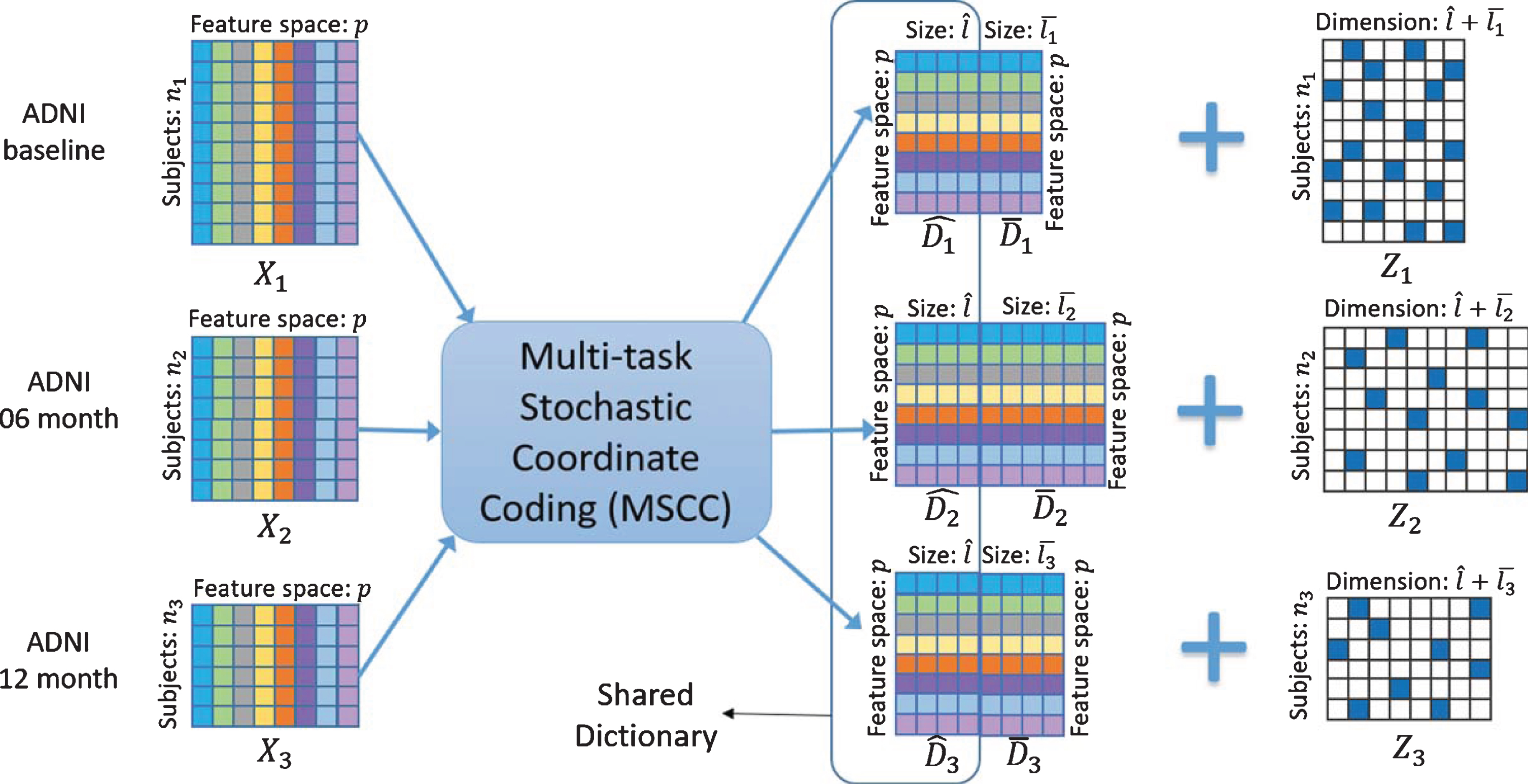
The initialization of dictionaries in MSCC is critical to the entire learning process. We propose a random patch method to initialize the dictionaries from different tasks. The main idea is to randomly select l image patches from n subjects {x₁, x₂,…, x_n} to construct $D \in ℝ^{p \times ℓ}$ . In MSCC, the way we initialize ${\hat{D}}_{t}$ is to randomly select $\hat{ℓ}$ subjects’ features from feature matrices across different tasks {X₁,…, X_T}. Similarly, for the individual part of each dictionary, we randomly select $\bar{ℓ}$ subjects’ features from the corresponding matrix X_t to construct ${\bar{D}}_{t}$ .

Fig. 4

Illustration of the learning process of MSCC on ADNI datasets from multiple tasks.

Algorithm 2 Multi-task Sparse Coordinate Coding
Require: Samples from different tasks: { X ₁, X ₂, …, X _T},
$X_{T} \in ℝ^{p \times n_{t}}$
Ensure: Dictionaries and sparse codes for each tasks:
{ D ₁, …, D _T} and { Z ₁, …, Z _T}
1: for k = 1 to kdo
2: for each image patch x_t ( i ) ∈ X _t, i ∈ { 1 , …, n _t} and
t ∈ { 1 , …, T}.
3: Update ${\hat{D}}_{t}^{k} : {\hat{D}}_{t}^{k} = Φ$ .
4: Update $Z_{t}^{k + 1} (i)$ and index set $I_{t}^{k + 1} (i)$ by a few steps of CCD:
5: $[Z_{t}^{k + 1} (i), I_{t}^{k + 1} (i)] = CCD ({\hat{D}}_{t}^{k}, {\bar{D}}_{t}^{k}, x_{t} (i), I_{t}^{k} (i), Z_{t}^{k} (i))$ .
6: Update the ${\hat{D}}_{t}$ and ${\bar{D}}_{t}$ by one step SGD:
7: $[{\hat{D}}_{t}^{k + 1}, {\bar{D}}_{t}^{k + 1}] = SGD ({\hat{D}}_{t}^{k}, {\bar{D}}_{t}^{k}, x_{t} (i), I_{t}^{k + 1} (i), Z_{t}^{k + 1} (i))$ .
8: Normalize ${\hat{D}}_{t}^{k + 1}$ and ${\bar{D}}_{t}^{k + 1}$ based on the index set $I_{t}^{k + 1} (i)$ .
9: Update the shared dictionary $Φ : Φ = {\hat{D}}_{t}^{k + 1}$ .
10: end for
11: end for
12: end for

After initializing dictionary D_t for each time point, we set all the sparse codes Z_t to be zero in the beginning. The key steps of MSCC are summarized in Algorithm 2, k denotes the epoch number where k ∈ {1, …, 𝜅}, Φ represents the shared part of each dictionary D _t which is initialized by the random patch method. For each subject’s patch x _t (i) extracted from X _t, we learn the ith sparse code $Z_{i}^{k + 1} (i)$ from Z_t by several steps of Cyclic Coordinate Descent (CCD) [58]. Then we use learned sparse codes $Z_{t}^{k + 1} (i)$ to update the dictionaries ${\hat{D}}_{t}^{k + 1}$ and ${\bar{D}}_{t}^{k + 1}$ by one step Stochastic Gradient Descent (SGD) [59]. Since $Z_{i}^{k + 1} (i)$ is very sparse, we use the index set $I_{i}^{k + 1} (i)$ to record the location of non-zero entries in $Z_{i}^{k + 1} (i)$ to accelerate the update of sparse codes and dictionaries, Φ is updated in the end of kth interaction to ensure ${\hat{D}}_{t}^{k + 1}$ is the same among all the dictionaries.

After we pick an image patch x_t(i) from the sample x_t at the time point t, we fix the dictionary and update the sparse codes by following the ODL method [30]. Then the optimization problem we need to solve becomes the following equation:

$min_{Z_{t} (i)} F (Z_{t} (i)) = \frac{1}{2} ∥ x_{t} (i) - Z_{t} (i) ∥_{2}^{2} + λ ∥ Z_{t} (i) ∥_{1}$ (2)

It is known as the Lasso problem [43]. Coordinate descent [58] is known as one of the state-of-the-art methods for solving this problem. In this study, we perform the CCD to optimize Eq. (2). Empirically, the iteration may take thousands of steps to converge. It is time-consuming in the optimization process of dictionary learning. However, we observe that after a few steps, the support of the coordinates, i.e., the locations of the non-zero entries in Z_t(i), becomes very stable, usually after less than ten steps. In this study, we perform P steps CCD to generate the non-zero index set $I_{t}^{k + 1}$ , recording the non-zero entry of $Z_{t}^{k + 1} (i)$ . Then we perform S steps CCD to update the sparse codes only on the non-zero entries of $Z_{t}^{k + 1} (i)$ , accelerating the learning process significantly. SCC [60, 61] employs a similar strategy to update the sparse codes in a single task. For the multi-task learning, we summarize the updating rules as follows:

Perform P steps CCD to update the locations of the non-zero entries $I_{t}^{k + 1} (i)$ and the model $Z_{t}^{k + 1} (i)$ .

Perform S steps CCD to update the $Z_{t}^{k + 1} (i)$ in the index of $I_{t}^{k + 1} (i)$ .

The detailed optimization procedure [32 , 61] is reported in Supplementary Material B.

Performance evaluation protocol

To evaluate the proposed framework, we randomly split the data into training and testing sets using an 8 : 2 ratio, i.e., models were constructed on 80% of the data and evaluated on the remaining 20% of the data. We also used 10-fold cross validation to select key parameters and avoid data bias during the training. Lastly, we evaluated the overall prediction performance using normalized mean square error (nMSE), weighted correlation coefficient (wR), and root mean square error (rMSE) for task-specific regression performance measures [17]. The three performance measures are defined as follows:

$\begin{matrix} nMSE (Y, \hat{Y}) = \frac{\sum_{i = 1}^{t} ∥ Y_{i} - {\hat{Y}}_{i} ∥_{2}^{2} / σ (Y_{i})}{\sum_{i = 1}^{t} n_{i}}, \\ wR (Y, \hat{Y}) = \frac{\sum_{i = 1}^{t} Corr (Y_{i}, {\hat{Y}}_{i}) n_{i}}{\sum_{i = 1}^{t} n_{i}}, \\ rMSE (y, \hat{y}) = \sqrt{\frac{∥ y - \hat{y} ∥_{2}^{2}}{n}} . \end{matrix}$ (3)

For nMSE and wR, Y_i is the ground truth of target task i and ${\hat{Y}}_{i}$ is the corresponding predicted value, σ (Y_i) is the standard deviation of Y_i, Corr is the Pearson correlation coefficient between two vectors and n_i is the number of subjects of task i. For rMSE, y is the ground truth of the target at a single task and ${\hat{y}}_{i}$ is the corresponding prediction by a prediction model. The smaller nMSE and rMSE, as well as the bigger wR mean the better prediction performances, nMSE and wR are used to evaluate the overall performances of the proposed system across multiple times points, rMSE is used to evaluate CNN-MSCC performance of each time point. We reported the mean and standard deviation based on 40 iterations of experiments on different splits of data. We compared the proposed model with seven other methods, which are as follows:

CNN-R: CNN learned surface feature without transfer learning, followed by Lasso regression.

MSCC-R: The proposed multi-task dictionary learning algorithm followed by Lasso regression.

OLSC-R: The single-task dictionary learning [30] followed by Lasso regression.

cFSGL: A multi-task algorithm called convex fused sparse group Lasso [17].

L21: A multi-task algorithm called L_2,1, norm regularization with least square loss [62].

Lasso: A single task method called Lasso regression [43].

Ridge: A single task method called Ridge regression [63].

Paired sample t-test was applied to compare performances (rMSE/nMSE and wR) between CNN-MSCC and seven other similar methods [64] and the statistical p values were corrected for false discovery rate (FDR) [65].

RESULTS

This section explains how to configure key parameters of the proposed system CNN-MSCC and provides performance comparisons between CNN-MSCC and other state-of-the-art methods.

We designed two different experiments to validate our proposed CNN-MSCC framework. In the first experiment (Experiment I), we applied CNN-MSCC to predict MMSE/ADAS-Cog scores of 24-months using HP image patches of baseline, 6-months, and 12-months. In the second experiment (Experiment II), we applied the CNN-MSCC to predict MMSE/ADAS-Cog scales of multi-time slots (6-months, 12-months, and 24-months) using image patches of baseline multi-ROIs (hippocampal/ventricle mTBM and cortical thickness). Comparison analyses were performed between CNN-MSCC and seven other similar methods in each experiment. To fit the pre-trained CNN model, patches of size 50×50 are extracted and resized to size of 227*227 input sample. There are either HP patches from multi-time slots (Experiment I) or three kinds of baseline structural patches (Experiment II). The image patch amount of each time point and structural measure are shown in Table 3.

Table 3

The image patch amounts of two experimental datasets

	Baseline	6-months	12-months
Longitudinal Hippocampal patches (individual patch number * subjects)	220968 (264 * 837)	193512 (264 * 733)	178464 (264 * 676)
	Hippocampal surfaces	Ventricular surfaces	Cortical thickness
Three baseline structural patches (individual patch number * subjects)	220968 (264 * 837)	2867562 (3426 * 837)	1504926 (1798 * 837)

Key parameter estimation

In this work, we estimate two key parameters of CNN-MSCC on longitudinal HP image patches and then use the optimized parameters throughout the paper.

The first key parameter is the amount pre-trained CNN layers for transferring learning. In this work, we aimed to get feature maps related with AD from image patch-based features using the well pre-trained CNN. With the transfer learning technique, the AlexNet architecture pre-trained on the ImageNet dataset [66] was tested on longitudinal HP image patches. CNN consists of multiple layers of feature maps, and each layer is a different representation of the input data. We used the HP image patches of three time points (baseline, 6-months, and 12-months) as inputs to predict MMSE/ADAS-Cog scales of 24-months. We studied their performances when working with different network layers (detailed in Table 2) of CNN-MSCC.

To verify the role of MSCC part, we also compared the performance of CNN-MSCC with the performance without MSCC part (CNN-R). The results are provided in Fig. 5. We observed that both CNN-MSCC and CNN-R with 6 network layers outperformed the others measured by rMSE. The discriminative power increases from the 4 to 6 layers, and then drops afterwards as the depth of network increases. One reasonable explanation about this observation is the lower layers do not fully capture the surface features and the higher layers captured features that overfit to the training image patches. Therefore, in this paper, we used the 6th layer’s features (4096) as the number of rows for all the dictionaries. Additionally, we also noted that CNN-MSCC outperformed CNN-R with different layer settings. It indicates that MSCC part helps to improve the prediction performance.

Fig. 5

Comparison of 24-months’ MMSE/ADAS-Cog prediction models with different CNN layers (both with and without MSCC part—CNN-MSCC versus CNN-R), in terms of root mean square error (rMSE) on hippocampal patches of baseline, 6-months, and 12-months. MMSE, Mini-Mental State Examination; ADAS-Cog, Alzheimer’s Disease Assessment Scale-Cognitive Subscale; CNN, Convolutional Neural Network; MSCC, Multi-task Stochastic Coordinate Coding; CNN-R, CNN-Regression.

The second key parameter is the proportions of common and individual parts in the dictionary of MSCC algorithm. The dictionary of MSCC algorithm includes common and individual parts for considering the constant and varied features of multi-task learning. It is necessary to evaluate the optimal proportions of the two parts in the dictionary. We still used the longitudinal HP image patches of three time points (baseline, 6-months, and 12-months) as inputs to predict MMSE/ADAS-Cog scales of 24-months and adopted 6-layers of CNN in the proposed algorithm. We set the dictionary size to be 2000 and partitioned the dictionary by different proportions: 250 : 1750, 500 : 1500, 1000 : 1000, 1500 : 500, and 1750 : 250, where the left number is the size of common part while the right number is the size of individual part for each dictionary. To verify the role of CNN part of the proposed method, we also calculated the performance of an algorithm MSCC-R without the CNN part. Figure 6 shows the rMSEs as the performance measures of two methods MSCC-R and CNN-MSCC on the longitudinal HP data. The rMSEs of MMSE/ADAS-Cog scales are lowest when we divide the dictionary in half. So, in all experiments, we use the ratio of 1000 : 1000 as the proportion of common and individual parts for all the dictionaries. Additionally, we observed that CNN-MSCC outperformed MSCC-R with different dictionary proportion settings. This indicates that CNN part also helps to improve the prediction performance. So, the combination of optimized CNN and MSCC is expected to have a promising performance on AD progression prediction. In the follow-up experiments, we will further validate this expectation.

Fig. 6

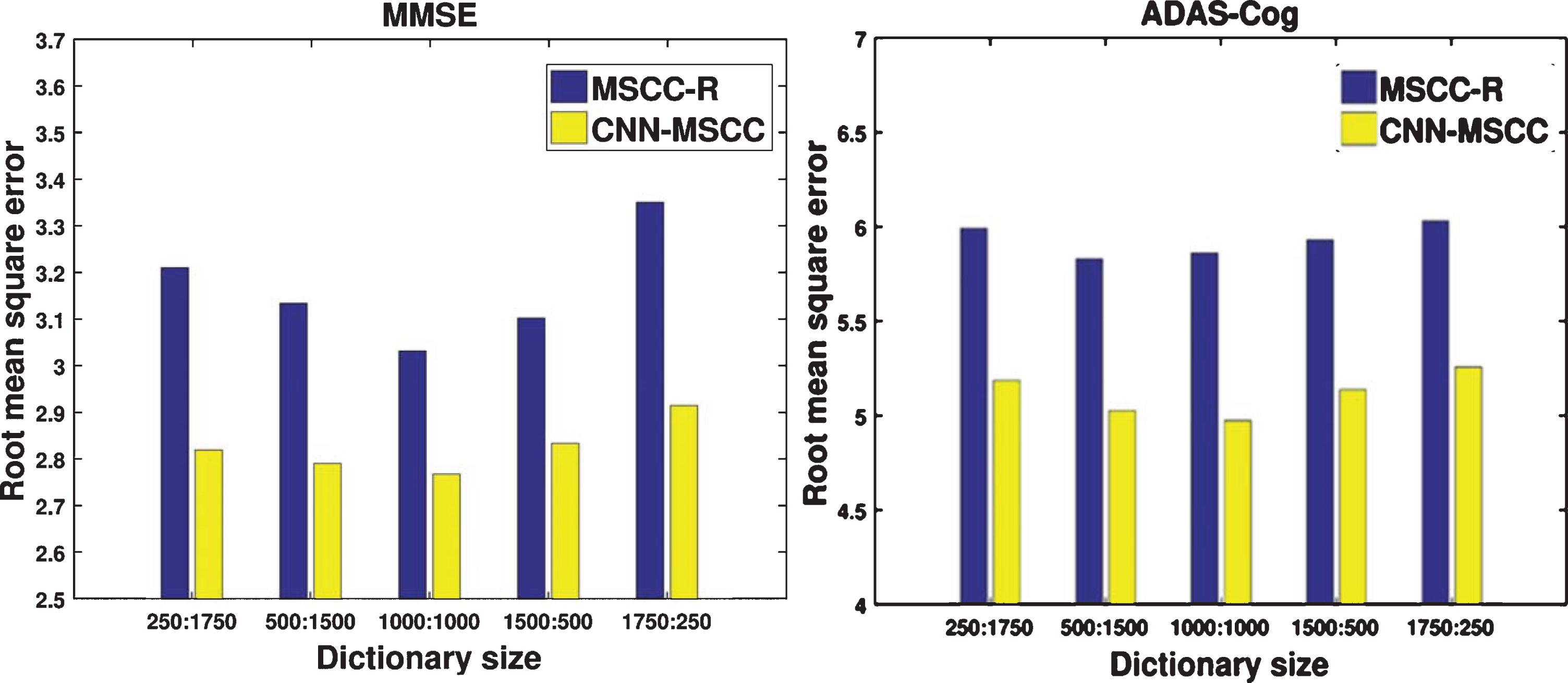
Comparison of 24-months’ MMSE/ADAS-Cog prediction performances with different dictionary settings of MSCC, in terms of root mean square error (rMSE) on hippocampal patches of baseline, 6-months and 12-months. MMSE, Mini-Mental State Examination; ADAS-Cog, Alzheimer’s Disease Assessment Scale-Cognitive Subscale; CNN, Convolutional Neural Network; MSCC-R, Multi-task Stochastic Coordinate Coding Regression.

Experiment I: CNN-MSCC on longitudinal HP surface patch features

Studies demonstrate that the hippocampal structure is a primary biomarker in the longitudinal structural MRI analysis of AD progression [11 , 67–70] and significant hippocampal deformations related with AD pathology can be detected even before observing obviously lower MMSE/ADAS-Cog scores [10 , 72]. In Experiment I, we used previous longitudinal HP patches (baseline, 6-months, and 12-months) to predict future MMSE/ADAS-Cog scales at the 24-months point. Image patches with size 50×50 were extracted from individual hippocampal mTBM feature maps of three tasks (baseline, 6-months, and 12-months), and we had 220968, 193512, and 178464 individual HP image patches for three tasks respectively. Using these image patches as the input of CNN-MSCC, we got three sets of feature sparse codes of baseline, 6-months, and 12-months. We used individual 12-months sparse codes learned by CNN-MSCC as Lasso design matrices to train and test the 24-months MMSE/ADAS-Cog scales with 8 : 2 subjects ratio, because the 12-months sparse codes contain both common features along with time points (baseline, 6-months, and 12-months) and task-specific features of 12-months. Figure 7 shows scatter plots of CNN-MSCC for the predicted values versus the actual values for MMSE/ADAS-Cog on the testing data.

Fig. 7

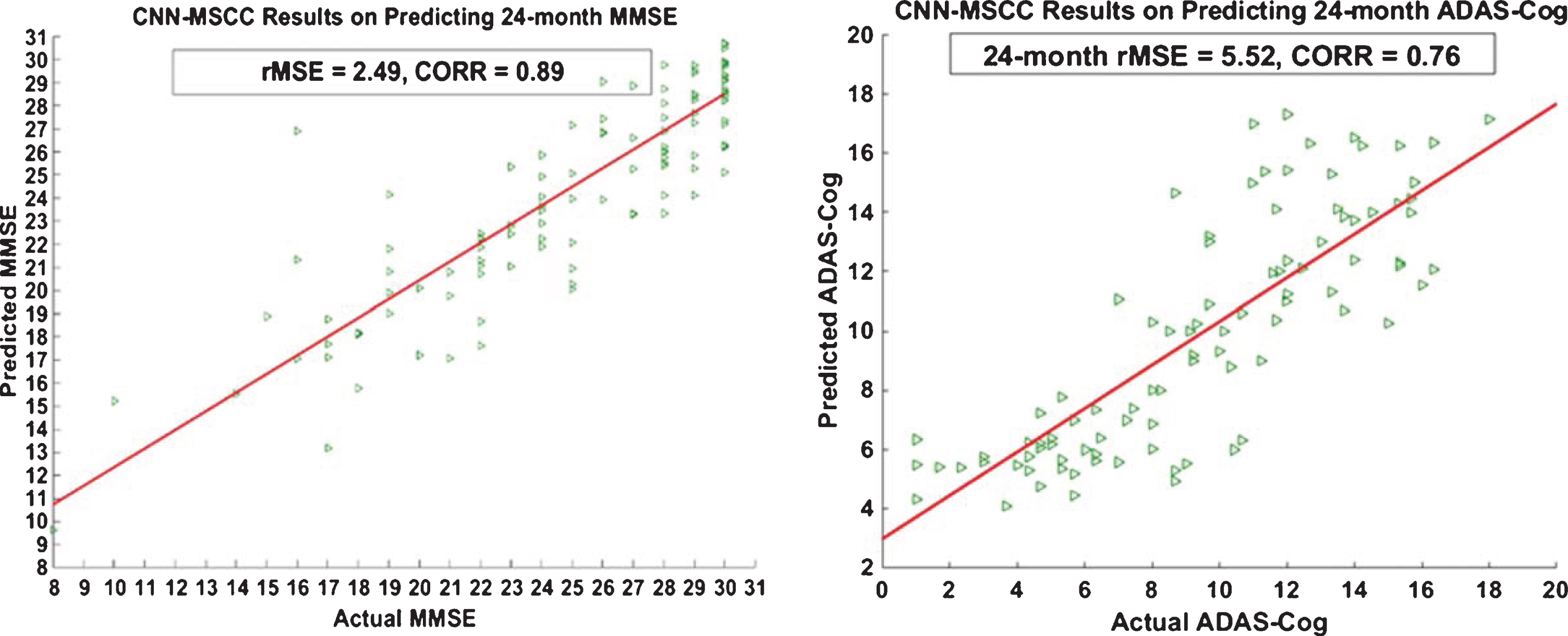
Scatter plots of actual versus predicted MMSE/ADAS-cog values of 24-months using CNN-MSCC based on hippocampal patches of baseline, 6-months, and 12-months. MMSE, Mini-Mental State Examination; ADAS-Cog, Alzheimer’s Disease Assessment Scale-Cognitive Subscale; CNN, Convolutional Neural Network; MSCC, Multi-task Stochastic Coordinate Coding; rMSE, root mean square error; CORR, Correlation coefficients.

To estimate the performance of CNN-MSCC on this application, we randomly split the training data and testing data as the 8 : 2 ratio and ran 40 iterations of each method, then we could apply paired sample t-test with lower-tailed hypothesis to compare the rMSEs performances of CNN-MSCC with seven other similar methods on the longitudinal HP dataset. All the p values were corrected by FDR. The rMSEs of 24-months MMSE/ADAS-Cog scale predictions are shown in Fig. 8. Statistical results indicate that, for MMSE scale predictions, CNN-MSCC has significantly smaller rMSEs (p < 0.05) compared to CNN-R, OLSC-R, cFSGL, L21, Lasso, and Ridge, while there is no significant rMSEs difference (p = 0.3459) for CNN-MSCC versus MSCC-R. For ADAS-Cog scale predictions, CNN-MSCC has significantly smaller rMSEs (p < 0.05) compared to all the other methods. All the eight methods demonstrate that the rMSEs of MMSE predictions are better than ADAS-Cog prediction.

Fig. 8

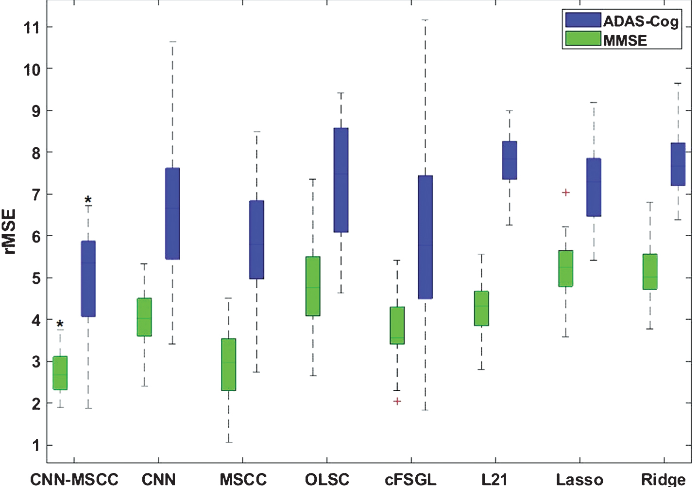
Comparison analysis of our proposed method and seven other similar methods on 24-months MMSE/ADAS-Cog scale prediction performances using hippocampal image patches of baseline, 6-months, and 12-months in terms of root mean square error (rMSE). Paired sample t-test was applied to estimate the significant outperformances of the proposed method CNN-MSCC. The asterisk above green boxplot shows that, for MMSE scale predictions, CNN-MSCC has significantly smaller (p < 0.05, corrected) rMSEs compared to CNN-R, OLSC-R, cFSGL, L21, Lasso, and Ridge, while there is no significant rMSEs difference for the contrast of CNN-MSCC versus MSCC-R. The asterisk above blue boxplot shows that, for ADAS-Cog scale predictions, CNN-MSCC has significantly smaller rMSEs (p < 0.05, corrected) compared to all other methods.

Experiment II: CNN-MSCC on multiple baseline cortical structural surface patch features

Ventricular mTBM and cortical thickness are another two important biomarkers for tracking the AD progression [6 , 73]. In Experiment II, we used the baseline structural image patches, including hippocampal mTBM features, ventricular mTBM features, and cortical thickness of 837 subjects to predict the MMSE/ADAS-Cog variations of future time points (6-months, 12-months, and 24-months). After preprocessing these MRI data, we have 220968, 2867562, and 1504926 individual image patches corresponding to three kinds of baseline structural measures respectively. Using the CNN-MSCC framework, we got three sets of feature sparse codes. Since each subject has three sparse codes, we combined these three sparse codes as Lasso design matrix to train and test the 6-months, 12-months, and 24-months MMSE/ADAS-Cog scales with 8 : 2 subjects’ ratio. This process was repeated 40 times. Figure 9 shows the boxplots of wRs between the predicted and the actual MMSE/ADAS-Cog scales of 6-months, 12-months, and 24-months. Using paired t-test with higher-tailed hypothesis between wRs of different time points, we found wRs on MMSE/ADAS-Cog score predictions of 24-months are significantly higher (p < 0.05) than wRs of 6-months and 12-months. These improved wRs on 24-months benefited from MSCC method to iteratively learn features from previous time points.

Fig. 9

Weighted correlation coefficient (wR) between predicted and actual MMSE/ADAS-Cog scales of 6-months, 12-months, and 24-months (M06, M12, and M24) on testing data using CNN-MSCC based on baseline multi-cortical image batches. Paired sample t-test was applied to estimate the significant outperformances on MMSE/ADAS-Cog scale predictions of 24-months. The asterisks above blue boxplots show that wRs on MMSE/ADAS-cog score predictions of 24-months are significantly higher (p < 0.05) than wRs of 6-months and 12-months.

Then we further compared our results with those of seven other state-of-the-art methods on the baseline multi-cortical dataset. Similarly, as in previous experiments, we randomly split the baseline training data and testing data as the 8 : 2 ratio and ran 40 iterations of each method, then we could apply paired sample t-test with lower-tailed hypothesis to compare the rMSE/nMSE performances and with higher-tailed hypothesis to compare wR performances of CNN-MSCC with seven other similar methods. Figure 10 shows the comparison results of our proposed method and seven other similar methods on longitudinal MMSE/ADAS-Cog prediction performances using baseline image patches of multiple ROIs in terms of normalized mean square error (nMSE, see Fig. 10a), weighted correlation coefficient (wR, see Fig. 10b) and root mean square error (rMSE, see Fig. 10c) at 6-months, 12-months, and 24-months (M06, M12, and M24). With paired sample t-test and FDR correction, we observed CNN-MSCC significantly outperform other similar methods with smaller (p < 0.05, corrected) rMSEs/nMSEs and higher (p < 0.05, corrected) wRs on future MMSE/ADAS-Cog scale predictions. Additionally, all the methods show apparently lower nMSE/rMSE when predict MMSE scales compared to predict ADAS-Cog scales. That is, neuroimaging features have closer relationship with MMSE scales compared to ADAS-Cog scales. These results support our hypothesis that a combination of features from multiple ROIs may enhance the statistical power in future cognitive measure regression.

Fig. 10

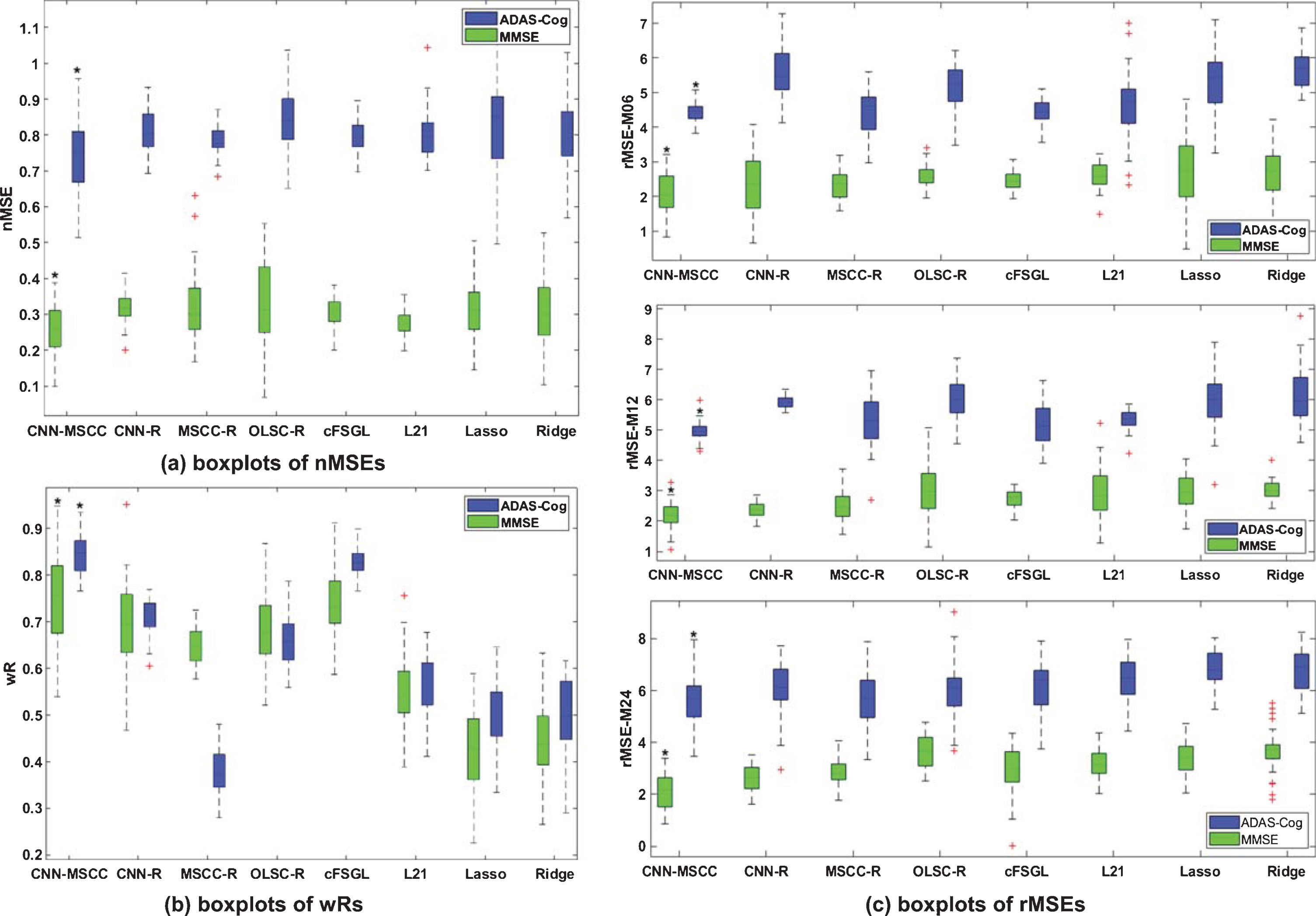
Comparison analysis of CNN-MSCC and seven other similar methods on longitudinal MMSE/ADAS-Cog prediction performances using baseline image patches of multiple ROIs in terms of normalized mean square error (nMSE) (a), weighted correlation coefficient (wR) (b), and root mean square error (rMSE) at 6-months, 12-months, and 24-months (M06, M12, and M24) (c). The asterisks above green boxplots and blue boxplots show that, for MMSE/ADAS-Cog scale predictions, CNN-MSCC has significantly smaller nMSEs/rMSEs (p < 0.05, corrected), and larger wRs (p < 0.05, corrected) compared to all other seven similar methods.

Sex/gender is one of the strongest predictors of AD, and women have twofold increased risk of AD than men after 65 years old [74, 75]. We applied CNN-MSCC to predict future MMSE/ADAS-Cog scales of males and females using baseline multi-task biomarkers. Paired sample t-test was applied to estimate performance differences between male and female groups. We observe that the female group has significantly smaller rMSEs (p < 0.05) on MMSE/ADAS-Cog scale predictions at 6-months compared to the male group, while no statistical difference is observed on rMSEs with 12-months and 24-months prediction and the overall nMSE and wR values (see Fig. 11). It may demonstrate that CNN-MSCC has a slightly higher effect size to predict female MMSE/ADAS-Cog scales than the male group. Our research show that female may have stronger connections between structural changes and future cognitive decline. It may provide some evidence supporting the existing research [74 –76] that reported the female is more vulnerable to AD than the male.

Fig. 11

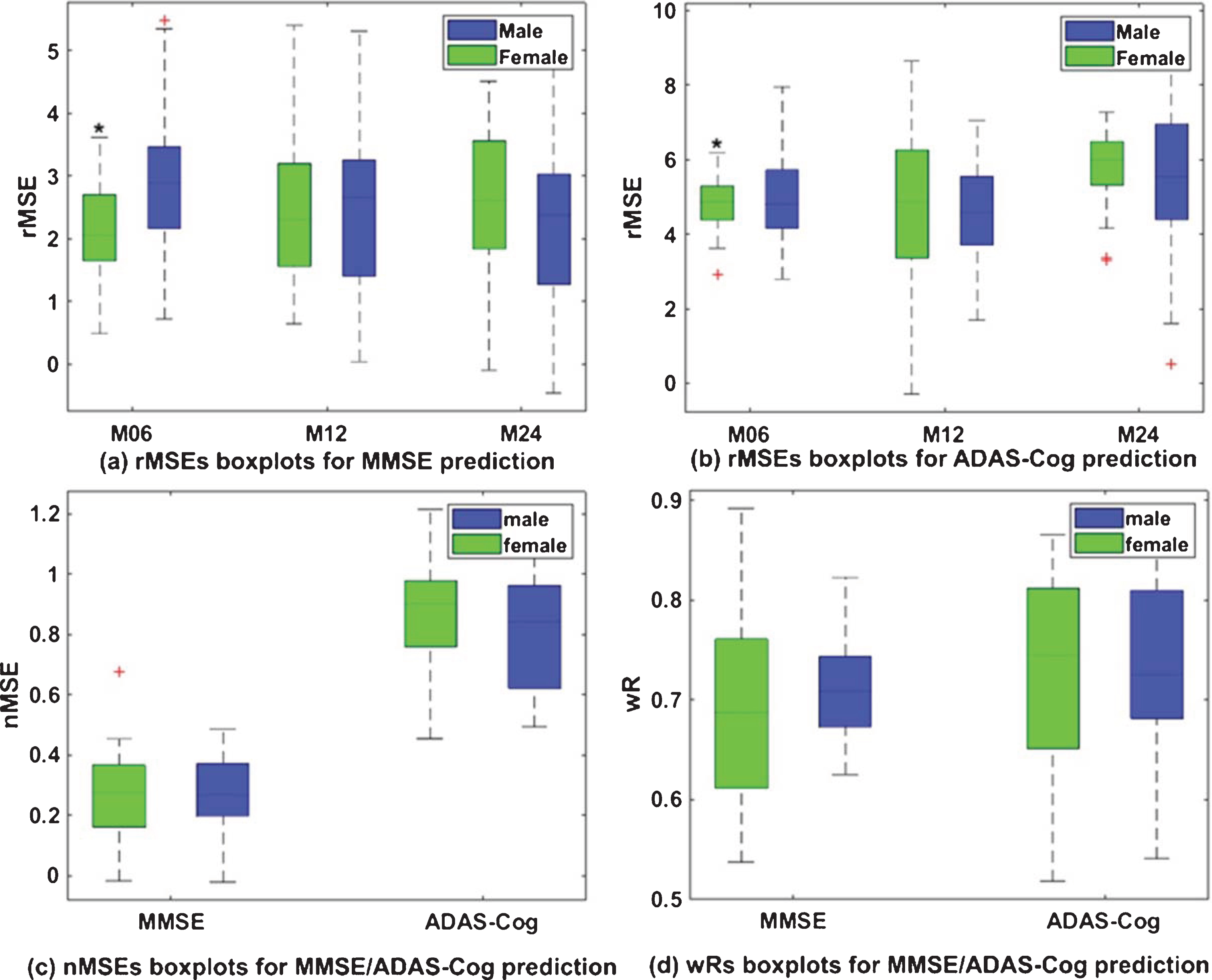
MMSE/ADAS-Cog prediction performances of male and female groups using the proposed CNN-MSCC method and baseline patches of multiple ROIs in terms of root mean square error (rMSE) at 6-months, 12-months, and 24-months (a) and (b), normalized mean square error (nMSE) (c), and weighted correlation coefficient (wR) (d). The asterisks above green boxplots in (a) and (b) show that female group have significantly smaller rMSEs (p < 0.05) on MMSE/ADAS-Cog scale predictions at 6-months compared to the male group.

DISCUSSION

This work has two main findings. First, we have demonstrated a novel system that integrates deep transfer learning and multi-task sparse coding research for enhanced AD progression modeling. CNN [24, 25] is good at extracting accurate neuroimaging characteristics of special neurodegenerative disease and the extracted neuroimaging features are in a high dimension as opposed to small sample size as known as “large p, small n” problem. While our proposed multi-task learning method MSCC can represent these high dimensional features and jointly analyze multi-task sparse features. One of the major discoveries of the current work is that the integration of both methods achieves improved statistical power. To the best of our knowledge, CNN-MSCC is the first deep model transfer learning from the large scale annotated natural images to brain surface statistics. Second, the surface mTBM, which is computed from the conformal grid and carries rich information on local surface geometry, is applicable to deep models for AD progressive prediction. Although surface-based morphometry achieved great success in population-based analyses to discover the general trend of disease burden and progression [6 , 77–79], few studies have investigated the use of surface-based morphometry features for brain disease diagnosis on an individual basis [80 –82]. This work validated the feasibility of surface mTBM [83], as imaging biomarkers for prediction of future MMSE/ADAS-Cog scales decline. This discovery is in line with several of our prior studies [6, 80]. The newly combined surface statistics practically encode a great deal of neighboring intrinsic geometry information that would otherwise be inaccessible or overlooked. The surface-based computer-aided diagnosis research may become more powerful by adopting these patch analysis-based multivariate statistics.

CNNs are considered as one of the most successful deep models for identifying, classifying, and quantifying patterns in medical images [53, 84]. There are still relatively few CNN studies on AD diagnosis due to limited training data. Transfer learning technique has proven to be a highly effective technique for addressing a lack of data in AD research domain and it leverages data from another domain. ImageNet includes millions of labeled natural images [54]. However, because of the substantial differences between natural and medical images, transfer learning is unsuitable to be applied directly [66]. Studies of [26, 66] demonstrated that fine-tuning the transferred CNNs on medical images could decrease overfitting of the pre-trained CNNs and was a practical way to reach the best performance for the medical image application at hand. Therefore, in this study, we pre-trained CNN structures on ImageNet database. After we pre-trained the CNN model on the ImageNet dataset, we removed the last fully connected layer (this layer’s outputs are the 1000 class scores for ImageNet). The dimension of ImageNet image is 227*227*3, while the dimension of our mTBM patch features is 50*50*3. We rescaled the surface mesh features to 227*227*3. Then the CNN on the surface mesh features was fine-tuned. Our results demonstrate that the transferred CNNs with optimal layers are capable to extract higher level features from image-patches of biomarkers and gain performance improvement for AD progressing modeling.

After using CNN with transfer learning technique, image patches of biomarkers were transformed to high dimensional feature maps. On one hand, to address the problem of high dimensional feature maps derived from small number of image patches, it is necessary to apply the sparse coding method to generate a small number of basis vectors termed dictionary to represent high dimensional features effectively and concisely [30 , 85]. On the other hand, multi-task sparse features contain complementary information for tracking AD progression measured by MMSE/ADAS-Cog scales [17, 18], so we need to effectively integrate these features together. Previous studies concatenated different kinds of features into a longer feature vector or applied multi-task learning method to fuse them together [18]. The study of [86, 87] reported that multi-task learning method performed better than feature concatenation method. However, if there is no latent common information shared by the same subject during different time points [17], only one dictionary from multiple-kernel method is not enough to show the variation among features from different time points. To address this challenge, we integrate the idea of multi-task learning into the online dictionary learning method [17 , 88] and propose the novel dictionary learning algorithm MSCC to learn multi-task sparse codes of subjects.

In our proposed model, we innovatively introduce the common part of dictionaries to capture the interrelationships between multi-task learning. As expected, CNN-MSCC outperformed several similar methods. To verify the common part role of multi-task dictionary, we tested the performances of CNN-MSCC versus CNN-separate task stochastic coordinate coding (CNN-STSC) that is without the common dictionary part. As shown in Fig. 12, CNN-MSCC with common dictionary part outperforms CNN-STSC without common dictionary part with significantly smaller rMSEs (p < 0.05) on MMSE scale predictions at three time points, with significantly smaller rMSEs (p < 0.05) on ADAS-Cog scale predictions at 6-months and 12-months, and with significantly larger wRs (p < 0.05) on ADAS-Cog scale predictions. The experimental results validated the gained statistical power by adding the common part of dictionaries. However, we did not observe significant rMSE differences on ADAS-Cog scale predictions at 24-months. Neither did we have significant nMSE differences on MMSE/ADAS-Cog scale predictions, nor significant wRs differences on MMSE scale predictions. MMSE/ADAS-Cog scale predictions of 6-months are based on the common and individual sparse features at baseline, while MMSE/ADAS-Cog scales of 12-months are based on the updated common sparse features along with time points (baseline and 6-months) and task-specific features of 6-months. Similarly, MMSE/ADAS-Cog scales of 24-months are based on the updated common sparse features along with time points (baseline, 6-months, and 12-months) and task-specific features of 12-months. This accumulate learning capability makes the prediction performances at 6-months, 12-months, and 24-months stable.

Fig. 12

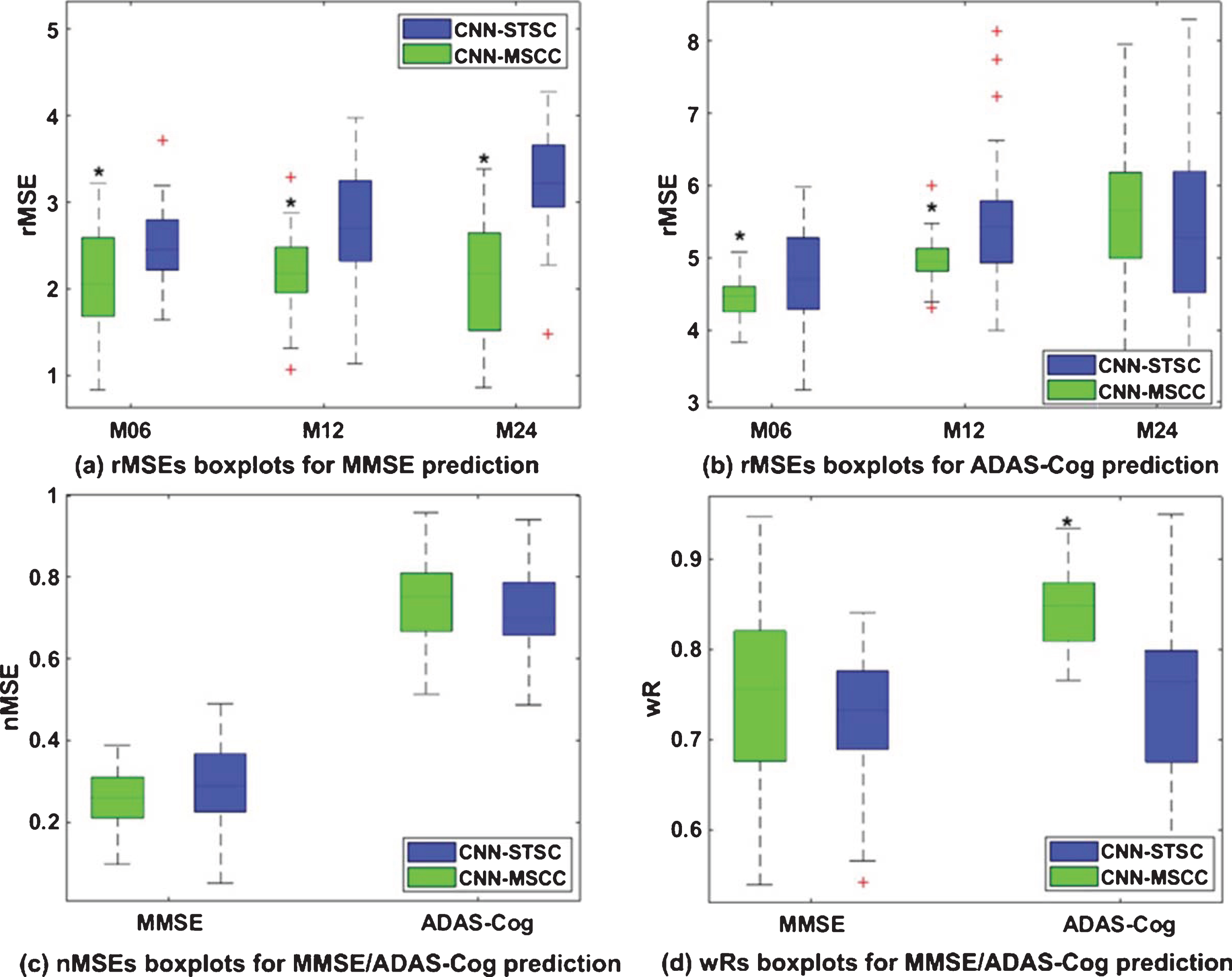
MMSE/ADAS-Cog prediction performances of CNN-MSCC and CNN-STSC on baseline patches of multiple ROIs in terms of root mean square error (rMSE) at 6-months, 12-months, and 24-months (a) and (b), normalized mean square error (nMSE) (c), and weighted correlation coefficient (wR) (d). The asterisks above green boxplots in (a) show that CNN-MSCC has significantly smaller rMSEs (p < 0.05) on MMSE scale predictions at three time points compared to CNN-STSC. The asterisks above green boxplots in (b) show that CNN-MSCC has significantly smaller rMSEs (p < 0.05) on ADAS-Cog scale predictions at 6-months and 12-months compared to CNN-STSC. The asterisk above the green boxplot in (d) shows that CNN-MSCC has significantly larger wRs (p < 0.05) on ADAS-Cog scale predictions compared to CNN-STSC.

Despite the promising experimental results, four caveats remain. First, this work aims to propose one comprehensive framework which includes CNN structure for image feature extractions, multi-task sparse coding algorithm for feature fusions and Lasso regression model for future cognitive scale predictions. We select AlexNet as the CNN part, the proposed automatic system outperformed 7 similar methods. In future work we would like to make comparison analysis of our proposed CNN-MSCC system based on kinds of well-known CNN structures, e.g., [89, 90], and expect the performance will be further improved. Second, transfer learning is still empirical and it lacks theoretical interpretations about what to transfer, how to transfer, and when to transfer [91]. It is still a mystery that machine learning systems can work on brain images while they were trained in other image domains. Even so, our work still demonstrated that the optimized CNN-MSCC model may extract reliable features for AD progression prediction and validate the feasibility to apply deep models on surface-based neuroimaging features. Third, as one of the useful data augmentation methods, transfer learning is not the only one to apply deep models in a small size dataset. Other ongoing methods, such as one-short/few shot learning, horizontal flips, random crops, and principal component analysis (PCA) are also promising ways to go [92 –96]. These strategies have been shown to capture important characteristics of natural and medical images. In our future work, we will keep exploring other data augmentation techniques to build deep neural networks with our surface features and compare their performances with the current transfer learning strategy. Fourth, our current model does not consider the temporal information, another work from our group enforces the sparsity of the sparse codebook representation by representing neighboring feature resemblance to improve the smoothness of prediction over the longitudinal neighboring time points. In future work, we will try to study the integration of the resemblant model with CNN and compare its performance with our current results.

Conclusions

This study proposed a novel deep learning system, CNN-MSCC, for AD clinical score predictions using multi-task image patches. By leveraging the transfer learning, we were able to apply a pre-trained CNN models to study brain images. We also innovatively proposed a multi-task stochastic coordinate coding (MSCC) algorithm for the multi-task learning which may integrate patched-based brain surface features from longitudinal or multiple ROIs. Our preliminary experimental results and performance analyses showed that our proposed system may outperform other similar methods and showed a promising accuracy for future MMSE/ADAS-Cog scale predictions. The proposed system may aid in expediting the diagnosis of AD progression, facilitating earlier clinical intervention and resulting in improved clinical outcomes.

In future, we will continue our deep model-based brain imaging research [97], optimize our methods and investigate their capability on longitudinal brain multimodality imaging datasets. There are various opportunities to generalize and enhance our current study for AD research. For example, there are many other neuroimaging biomarkers from modalities such as PET, functional MRI, magnetoencephalography, and electroencephalogram, which have been widely studied for AD diagnosis [98 –100]. Since our proposed system is capable to refine and fuse features from multi-task biomarkers so we may also fuse these data in our system. The current work applied the proposed CNN-MSCC model to predict AD progression measured by MMSE/ADAS-Cog scales successfully. We may investigate more AD clinical assessments, such as Functional Assessment Questionnaire, the Clock Test, and the Rey Auditory Verbal Learning Test [101]. The gained experience may shed new lights the correlation between brain images and various AD clinical assessments and eventually help set up standards for subject recruitments in AD clinical trials [102].

Footnotes

ACKNOWLEDGMENTS

Algorithm development and image analysis for this study was funded, in part, by the National Institute on Aging (RF1AG051710 to QD, JZ and YW, R01EB025032 to NL and YW, R01AG031581 and P30AG19610 to RJC), the National Science Foundation (IIS-1421165 to JZ and YW), and Arizona Alzheimer’s Consortium. We gratefully acknowledge the support of NVIDIA Corporation with the donation of the Tesla K40 GPU used for this research.

Data collection and sharing for this project was funded by the ADNI (National Institutes of Health Grant U01 AG024904) and DOD ADNI (Department of Defense award number W81XWH-12-2-0012). ADNI is funded by the National Institute on Aging, the National Institute of Biomedical Imaging and Bioengineering, and through generous contributions from the following: AbbVie, Alzheimer’s Association; Alzheimer’s Drug Discovery Foundation; Araclon Biotech; BioClinica, Inc.; Biogen; Bristol-Myers Squibb Company; CereSpir, Inc.; Cogstate; Eisai Inc.; Elan Pharmaceuticals, Inc.; Eli Lilly and Company; EuroImmun; F. Hoffmann-La Roche Ltd and its affiliated company Genentech, Inc.; Fujirebio; GE Healthcare; IXICO Ltd.; Janssen Alzheimer Immunotherapy Research & Development, LLC.; Johnson & Johnson Pharmaceutical Research & Development LLC.; Lumosity; Lundbeck; Merck & Co., Inc.; Meso Scale Diagnostics, LLC.; NeuroRx Research; Neurotrack Technologies; Novartis Pharmaceuticals Corporation; Pfizer Inc.; Piramal Imaging; Servier; Takeda Pharmaceutical Company; and Transition Therapeutics. The Canadian Institutes of Health Research is providing funds to support ADNI clinical sites in Canada. Private sector contributions are facilitated by the Foundation for the National Institutes of Health (http://www.fnih.org). The grantee organization is the Northern California Institute for Research and Education, and the study is coordinated by the Alzheimer’s Therapeutic Research Institute at the University of Southern California. ADNI data are disseminated by the Laboratory for Neuro Imaging at the University of Southern California.

Authors’ disclosures available online ().

The supplementary material is available in the electronic version of this article: .

References

Brookmeyer

, Johnson

, Ziegler-Graham

, Arrighi

(2007) Forecasting the global burden of Alzheimer’s disease. Alzheimers Dement 3, 186–191.

Rathore

, Habes

, Iftikhar

, Shacklett

, Davatzikos

(2017) A review on neuroimaging-based classification studies and associated feature extraction methods for Alzheimer’s disease and its prodromal stages. Neuroimage 155, 530–548.

Sperling

, Aisen

, Beckett

, Bennett

, Craft

, Fagan

, Iwatsubo

, Jack

Jr. , Kaye

, Montine

, Park

, Reiman

, Rowe

, Siemers

, Stern

, Yaffe

, Carrillo

, Thies

, Morrison-Bogorad

, Wagster

, Phelps

(2011) Toward defining the preclinical stages of Alzheimer’s disease: Recommendations from the National Institute on Aging-Alzheimer’s Association workgroups on diagnostic guidelines for Alzheimer’s disease. Alzheimers Dement 7, 280–292.

Saykin

, Shen

, Foroud

, Potkin

, Swaminathan

, Kim

, Risacher

, Nho

, Huentelman

, Craig

, Thompson

, Stein

, Moore

, Farrer

, Green

, Bertram

, Jack

, Weiner

(2010) Alzheimer’s Disease Neuroimaging Initiative biomarkers as quantitative phenotypes: Genetics core aims, progress, and plans. Alzheimers Dement 6, 265–273.

van de Pol

, van der Flier

, Korf

, Fox

, Barkhof

, Scheltens

(2007) Baseline predictors of rates of hippocampal atrophy in mild cognitive impairment. Neurology 69, 1491–1497.

Wang

, Song

, Rajagopalan

, An

, Liu

, Chou

Y-Y

, Gutman

, Toga

, Thompson

(2011) Surface-based TBM boosts power to detect disease effects on the brain: An N=804 ADNI study. Neuroimage 56, 1993–2010.

Mosconi

, Nacmias

, Sorbi

, De Cristofaro

, Fayazz

, Tedde

, Bracco

, Herholz

, Pupi

(2004) Brain metabolic decreases related to the dose of the ApoE e4 allele in Alzheimer’s disease. J Neurol Neurosurg Psychiatry 75, 370–376.

Mosconi

, Berti

, Glodzik

, Pupi

, De Santi

, de Leon

(2010) Pre-clinical detection of Alzheimer’s disease using FDG-PET, with or without amyloid imaging. J Alzheimers Dis 20, 843–854.

Jack

, Bennett

, Blennow

, Carrillo

, Dunn

, Haeberlein

, Holtzman

, Jagust

, Jessen

, Karlawish

, Liu

, Molinuevo

, Montine

, Phelps

, Rankin

, Rowe

, Scheltens

, Siemers

, Snyder

, Sperling

, Elliott

, Masliah

, Ryan

, Silverberg

(2018) NIA-AA Research Framework: Toward a biological definition of Alzheimer’s disease. Alzheimers Dement 14, 535–562.

10.

Dong

, Zhang

, Wu

, Li

, Schron

, McMahon

, Shi

, Gutman

, Chen

, Baxter

, Thompson

, Reiman

, Caselli

, Wang

(2019) Applying surface-based hippocampal morphometry to study APOE-E4 allele dose effects in cognitively unimpaired subjects. Neuroimage Clin 22, 101744.

11.

Frisoni

, Fox

, Jack

, Scheltens

, Thompson

(2010) The clinical use of structural MRI in Alzheimer disease. Nat Rev Neurol 6, 67–77.

12.

Reiter

, Nielson

, Durgerian

, Woodard

, Smith

, Seidenberg

, Kelly

, Rao

(2017) Five-year longitudinal brain volume change in healthy elders at genetic risk for Alzheimer’s disease. J Alzheimers Dis 55, 1363–1377.

13.

Sørensen

, Igel

, Pai

, Balas

, Anker

, Lillholm

, Nielsen

(2017) Differential diagnosis of mild cognitive impairment and Alzheimer’s disease using structural MRI cortical thickness, hippocampal shape, hippocampal texture, and volumetry. Neuroimage Clin 13, 470–482.

14.

Weston

, Nicholas

, Lehmann

, Ryan

, Liang

, Macpherson

, Modat

, Rossor

, Schott

, Ourselin

, Fox

(2016) Presymptomatic cortical thinning in familial Alzheimer disease: A longitudinal MRI study. Neurology 87, 2050–2057.

15.

Pettigrew

, Soldan

, Zhu

, Wang

, Moghekar

, Brown

, Miller

, Albert

(2016) Cortical thickness in relation to clinical symptom onset in preclinical AD. Neuroimage Clin 12, 116–122.

16.

Zhao

, Raichle

, Wen

, Benzinger

, Fagan

, Hassenstab

, Vlassenko

, Luo

, Cairns

, Christensen

, Morris

, Yablonskiy

(2017) In vivo detection of microstructural correlates of brain pathology in preclinical and early Alzheimer disease with magnetic resonance imaging. Neuroimage 148, 296–304.

17.

Zhou

, Liu

, Narayan

, Ye

(2013) Modeling disease progression via multi-task learning. Neuroimage 78, 233–248.

18.

Zhang

, Shen

(2012) Multi-modal multi-task learning for joint prediction of multiple regression and classification variables in Alzheimer’s disease. Neuroimage 59, 895–907.

19.

Vemuri

, Gunter

, Senjem

, Whitwell

, Kantarci

, Knopman

, Boeve

, Petersen

, Jack

(2008) Alzheimer’s disease diagnosis in individual subjects using structural MR images: Validation studies. Neuroimage 39, 1186–1197.

20.

Fan

, Resnick

, Wu

, Davatzikos

(2008) Structural and functional biomarkers of prodromal Alzheimer’s disease: A high-dimensional pattern classification study. Neuroimage 41, 277–285.

21.

Greenspan

, van Ginneken

, Summers

(2016) Guest Editorial. Deep learning in medical imaging: Overview and future promise of an exciting new technique. IEEE Trans Med Imaging 35, 1153–1159.

22.

Krizhevsky

, Sutskever

, Hinton

(2017) ImageNet classification with deep convolutional neural networks. Commun ACM 60, 84–90.

23.

Turaga

, Murray

, Jain

, Roth

, Helmstaedter

, Briggman

, Denk

, Seung

(2010) Convolutional networks can learn to generate affinity graphs for image segmentation. Neural Comput 22, 511–538.

24.

Hazlett

, Gu

, Munsell

, Kim

, Styner

, Wolff

, Elison

, Swanson

, Zhu

, Botteron

, Collins

, Constantino

, Dager

, Estes

, Evans

, Fonov

, Gerig

, Kostopoulos

, McKinstry

, Pandey

, Paterson

, Pruett

, Schultz

, Shaw

, Zwaigenbaum

, Piven

, IBIS Network; Clinical Sites; Data Coordinating Center; Image Processing Core; Statistical Analysis (2017) Early brain development in infants at high risk for autism spectrum disorder. Nature 542, 348–351.

25.

, Habes

, Wolk

, Fan

(2019) A deep learning model for early prediction of Alzheimer’s disease dementia based on hippocampal magnetic resonance imaging data. Alzheimers Dement 15, 1059–1070.

26.

Kermany

, Goldbaum

, Cai

, Valentim

CCS

, Liang

, Baxter

, McKeown

, Yang

, Wu

, Yan

, Dong

, Prasadha

, Pei

, Ting

, Zhu

, Li

, Hewett

, Dong

, Ziyar

, Shi

, Zhang

, Zheng

, Hou

, Shi

, Fu

, Duan

, Huu

VAN

, Wen

, Zhang

, Li

, Wang

, Singer

, Sun

, Xu

, Tafreshi

, Lewis

, Xia

, Zhang

(2018) Identifying medical diagnoses and treatable diseases by image-based deep learning. Cell 172, 1122–1131.e9.

27.

, Park

, Lee

, Hwang

(2019) Using transfer learning onwhole slide images to predict tumor mutational burden in bladder cancer patients. bioRxiv 554527; doi: 10.1101/554527.

28.

Lee

, Battle

, Raina

, Ng

(2006) Efficient sparse coding algorithms. In Advances in Neural Information Processing Systems, pp. 801–808.

29.

Zhang

, Stonnington

, Li

, Shi

, Bauer

, Gutman

, Chen

, Reiman

, Thompson

, Ye

, Wang

(2016) Applying sparse coding to surface multivariate tensor-based morphometry to predict future cognitive decline. In 2016 IEEE 13th International Symposium on Biomedical Imaging (ISBI) IEEE, pp. 646–650.

30.

Mairal

, Bach

, Ponce

, Sapiro

(2009) Online dictionary learning for sparse coding. In Proceedings of the 26th Annual International Conference on Machine Learning, pp. 689–696.

31.

Giger

(2018) Machine learning in medical imaging. J Am Coll Radiol 15, 512–520.

32.

Zhang

, Li

, Caselli

, Thompson

, Ye

, Wang

(2017) Multi-source multi-target dictionary learning for prediction of cognitive decline. Inf Process Med Imaging 10265, 184–197.

33.

Liu

, Zhang

, Adeli

, Shen

(2019) Joint classification and regression via deep multi-task multi-channel learning for Alzheimer’s disease diagnosis. IEEE Trans Biomed Eng 66, 1195–1206.

34.

Ferrarini

, Palm

, Olofsen

, van der Landen

, Jan Blauw

, Westendorp

RGJ

, Bollen

ELEM

, Middelkoop

HAM

, Reiber

JHC

, van Buchem

, Admiraal-Behloul

(2008) MMSE scores correlate with local ventricular enlargement in the spectrum from cognitively normal to Alzheimer disease. Neuroimage 39, 1832–1838.

35.

Cano

, Posner

, Moline

, Hurt

, Swartz

, Hsu

, Hobart

(2010) The ADAS-cog in Alzheimer’s disease clinical trials: Psychometric evaluation of the sum and its parts. J Neurol Neurosurg Psychiatry 81, 1363–1368.

36.

Weiner

, Veitch

, Aisen

, Beckett

, Cairns

, Green

, Harvey

, Jack

, Jagust

, Liu

, Morris

, Petersen

, Saykin

, Schmidt

, Shaw

, Shen

, Siuciak

, Soares

, Toga

, Trojanowski

; Alzheimer’s Disease Neuroimaging Initiative (2013) The Alzheimer’s Disease Neuroimaging Initiative: A review of papers published since its inception. Alzheimers Dement 9, e111–e194.

37.

Jack

Jr. , Bernstein

, Fox

, Thompson

, Alexander

, Harvey

, Borowski

, Britson

, Whitwell

, Ward

, Dale

, Felmlee

, Gunter

, Hill

DLG

, Killiany

, Schuff

, Fox-Bosetti

, Lin

, Studholme

, DeCarli

, Krueger

, Ward

, Metzger

, Scott

, Mallozzi

, Blezek

, Levy

, Debbins

, Fleisher

, Albert

, Green

, Bartzokis

, Glover

, Mugler

, Weiner

(2008) The Alzheimer’s disease neuroimaging initiative (ADNI): MRI methods. J Magn Reson Imaging 27, 685–691.

38.

Shi

, Thompson

, Wang

(2011) Human brain mapping with conformal geometry and multivariate tensor-based morphometry. In Lecture Notes in Computer Science (including subseries Lecture Notes in Artificial Intelligence and Lecture Notes in Bioinformatics), pp. 126–134.

39.

Lawrence

, Giles

, Tsoi

Ah Chung

, Back

(1997) Face recognition: A convolutional neural-network approach. IEEE Trans Neural Networks 8, 98–113.

40.

Fischl

(2012) FreeSurfer. Neuroimage 62, 774–781.

41.

Zhang

, Fan

, Li

, Thompson

, Ye

, Wang

(2017) Empowering cortical thickness measures in clinical diagnosis of Alzheimer’s disease with spherical sparse coding. In 2017 IEEE 14th International Symposium on Biomedical Imaging (ISBI 2017) IEEE, pp. 446–450.

42.

Zhang

, Shi

, Stonnington

, Li

, Gutman

, Chen

, Reiman

, Caselli

, Thompson

, Ye

, Wang

(2016) Hyperbolic space sparse coding with its application on prediction of Alzheimer’s disease in mild cognitive impairment. In International Conference on Medical Image Computing and Computer-Assisted Intervention, pp. 326–334.

43.

Tibshirani

(2018) Regression shrinkage and selection via the Lasso. J R Stat Soc Ser B 58, 267–288.

44.

Patenaude

, Smith

, Kennedy

, Jenkinson

(2011) A Bayesian model of shape and appearance for subcortical brain segmentation. Neuroimage 56, 907–922.

45.

Lorensen

, Cline

(1987) Marching cubes: A high resolution 3D surface construction algorithm. In ACM Siggraph Computer Graphics, pp. 163–169.

46.

Wang

, Lui

, Gu

, Hayashi

, Chan

, Toga

, Thompson

, Yau

S-T

(2007) Brain surface conformal parameterization using Riemann surface structure. IEEE Trans Med Imag 26, 853–865.

47.

Shi

, Thompson

, Gutman

, Wang

, Alzheimer’s Disease Neuroimaging Initiative (2013) Surface fluid registration of conformal representation: Application to detect disease burden and genetic influence on hippocampus. Neuroimage 78, 111–134.

48.

Chou

Y-Y

, Leporé

, Saharan

, Madsen

, Hua

, Jack

, Shaw

, Trojanowski

, Weiner

, Toga

, Thompson

(2010) Ventricular maps in 804 ADNI subjects: Correlations with CSF biomarkers and clinical decline. Neurobiol Aging 31, 1386–1400.

49.

Chung

, Dalton

, Shen

, Evans

, Davidson

(2007) Weighted Fourier series representation and its application to quantifying the amount of gray matter. IEEE Trans Med Imaging 26, 566–581.

50.

Suzuki

(2017) Overview of deep learning in medical imaging. Radiol Phys Technol 10, 257–273.

51.

Rumelhart

, Hinton

, Williams

(1986) Learning representations by back-propagating errors. Nature 323, 533–536.

52.

Mittal

(2020) A survey of FPGA-based accelerators for convolutional neural networks. Neural Comput Appl 32, 1109–1139.

53.

Litjens

, Kooi

, Bejnordi

, Setio

AAA

, Ciompi

, Ghafoorian

, van der Laak

JAWM

, van Ginneken

, Sánchez

(2017) A survey on deep learning in medical image analysis. Med Image Anal 42, 60–88.

54.

Deng

, Dong

, Socher

, Li

L-J

, Li

, Fei-Fei

(2009) Imagenet: A large-scale hierarchical image database. In 2009 IEEE Conference on Computer Vision and Pattern Recognition, pp. 248–255.

55.

Jia

, Shelhamer

, Donahue

, Karayev

, Long

, Girshick

, Guadarrama

, Darrell

(2014) Caffe. In Proceedings of the ACM International Conference on Multimedia -MM’14 ACM Press, NewYork, NewYork, USA, pp. 675–678.

56.

Lao

, Wang

, Shi

, Ceschin

, Nelson

, Panigrahy

, Leporé

(2016) Thalamic alterations in preterm neonates and their relation to ventral striatum disturbances revealed by a combined shape and pose analysis. Brain Struct Funct 221, 487–506.

57.

Wang

, Zhang

, Chaim

, Zanetti

M V

, Davatzikos

(2015) Classification of MRI under the presence of disease heterogeneity using multi-task learning: Application to bipolar disorder. In Medical Image Computing and Computer-Assisted Intervention–MICCAI 2015 Springer, pp. 125–132.

58.

Canutescu

, Dunbrack

(2003) Cyclic coordinate descent: A robotics algorithm for protein loop closure. Protein Sci 12, 963–972.

59.

Zhang

(2004) Solving large scale linear prediction problems using stochastic gradient descent algorithms. In Twenty-first international conference on Machine learning - ICML ’04. ACM Press, New York, p. 116.

60.

Lin

, Li

, Sun

, Lai

M-J

, Davidson

, Fan

, Ye

(2014) Stochastic coordinate coding and its application for drosophila gene expression pattern annotation. arXiv, 1407.8147.

61.

, Lin

, Li

, Zhang

, Zhao

, Jiang

, Guo

, Han

, Hu

, Guo

, Ye

, Liu

(2017) Task fMRI data analysis based on supervised stochastic coordinate coding. Med Image Anal 38, 1–16.

62.

Argyriou

, Evgeniou

, Pontil

(2008) Convex multi-task feature learning. Mach Learn 73, 243–272.

63.

Hoerl

, Kennard

(1970) Ridge regression: Biased estimation for nonorthogonal problems. Technometrics 12, 55–67.

64.

(2006) Paired-samples T-test. In Handbook of Univariate andMultivariate Data Analysis and Interpretation with SPSS. Chapman and Hall/CRC, pp. 47–50.

65.

Benjamini

, Hochberg

(1995) Controlling the false discovery rate: A practical and powerful approach to multiple testing. J R Stat Soc Ser B 57, 289–300.

66.

Tajbakhsh

, Shin

, Gurudu

, Hurst

, Kendall

, Gotway

, Liang

(2016) Convolutional neural networks for medical image analysis: Full training or fine tuning? . IEEE Trans Med Imaging 35, 1299–1312.

67.

Worker

, Dima

, Combes

, Crum

, Streffer

, Einstein

, Mehta

, Barker

, C. R. Williams

, O’daly

(2018) Test–retest reliability and longitudinal analysis of automated hippocampal subregion volumes in healthy ageing and Alzheimer’s disease populations. Hum Brain Mapp 39, 1743–1754.

68.

, Shi

, Gutman

, Baxter

, Thompson

, Caselli

, Wang

(2016) Influence of APOE genotype on hippocampal atrophy over time - An N=1925 surface-based ADNI study. PLoS One 11, e0152901.

69.

Jack

Jr. , Slomkowski

, Gracon

, Hoover

, Felmlee

, Stewart

, Xu

, Shiung

, O’Brien

, Cha

, Knopman

, Petersen

(2003) MRI as a biomarker of disease progression in a therapeutic trial of milameline for AD. Neurology 60, 253–260.

70.

Thompson

, Hayashi

, Sowell

, Gogtay

, Giedd

, Rapoport

, de Zubicaray

, Janke

, Rose

, Semple

, Doddrell

, Wang

, van Erp

TGM

, Cannon

, Toga

(2004) Mapping cortical change in Alzheimer’s disease, brain development, and schizophrenia. Neuroimage 23, S2–S18.

71.

Cacciaglia

, Molinuevo

, Falcón

, Brugulat-Serrat

, Sánchez-Benavides

, Gramunt

, Esteller

, Morán

, Minguillón

, Fauria

, Gispert

(2018) Effects of APOE-ɛ4 allele load on brain morphology in a cohort of middle-aged healthy individuals with enriched genetic risk for Alzheimer’s disease. Alzheimers Dement 14, 902–912.

72.

Operto

, Cacciaglia

, Grau-Rivera

, Falcon

, Brugulat-Serrat

, Ródenas

, Ramos

, Morán

, Esteller

, Bargalló

, Molinuevo

, Gispert

(2018) White matter microstructure is altered in cognitively normal middle-aged APOE-ɛ4 homozygotes. Alzheimers Res Ther 10, 48.

73.

Chung

, Robbins

, Dalton

, Davidson

, Alexander

, Evans

(2005) Cortical thickness analysis in autism with heat kernel smoothing. Neuroimage 25, 1256–1265.

74.

Vest

, Pike

(2013) Gender, sex steroid hormones, and Alzheimer’s disease. Horm Behav 63, 301–307.

75.

Podcasy

, Epperson

(2016) Considering sex and gender in Alzheimer disease and other dementias. Dialogues Clin Neurosci 18, 437–446.

76.

Nebel

, Aggarwal

, Barnes

, Gallagher

, Goldstein

, Kantarci

, Mallampalli

, Mormino

, Scott

, Yu

, Maki

, Mielke

(2018) Understanding the impact of sex and gender in Alzheimer’s disease: A call to action. Alzheimers Dement 14, 1171–1183.

77.

Thompson

(1998) Cortical variability and asymmetry in normal aging and Alzheimer’s disease. Cereb Cortex 8, 492–509.

78.

Dale

, Fischl

, Sereno

(1999) Cortical surface-based analysis. Neuroimage 9, 179–194.

79.

Chung

, Robbins

, Evans

(2005) Unified statistical approach to cortical thickness analysis. In Biennial International Conference on Information Processing in Medical Imaging, pp. 627–638.

80.

Wang

, Yuan

, Shi

, Greve

, Ye

, Toga

, Reiss

, Thompson

(2013) Applying tensor-based morphometry to parametric surfaces can improve MRI-based disease diagnosis. Neuroimage 74, 209–230.

81.

Sun

, van Erp

TGM

, Thompson

, Bearden

, Daley

, Kushan

, Hardt

, Nuechterlein

, Toga

, Cannon

(2009) Elucidating a magnetic resonance imaging-based neuroanatomic biomarker for psychosis: Classification analysis using probabilistic brain atlas and machine learning algorithms. Biol Psychiatry 66, 1055–1060.

82.

Gutman

, Wang

, Morra

, Toga

, Thompson

(2009) Disease classification with hippocampal shape invariants. Hippocampus 19, 572–578.

83.

Wang

, Zhang

, Gutman

, Chan

, Becker

, Aizenstein

, Lopez

, Tamburo

, Toga

, Thompson

(2010) Multivariate tensor-based morphometry on surfaces: Application to mapping ventricular abnormalities in HIV/AIDS. Neuroimage 49, 2141–2157.

84.

Shen

, Wu

, Suk

H-I

(2017) Deep learning in medical image analysis. Annu Rev Biomed Eng 19, 221–248.

85.

Donoho

, Elad

(2003) Optimally sparse representation in general (nonorthogonal) dictionaries via l1 minimization. Proc Natl Acad Sci U S A 100, 2197–2202.

86.

Hinrichs

, Singh

, Xu

, Johnson

(2011) Predictive markers for AD in a multi-modality framework: An analysis of MCI progression in the ADNI population. Neuroimage 55, 574–589.

87.

Zhang

, Wang

, Zhou

, Yuan

, Shen

(2011) Multimodal classification of Alzheimer’s disease and mild cognitive impairment. Neuroimage 55, 856–867.

88.

Zhang

, Shen

(2012) Predicting future clinical changes of MCI patients using longitudinal and multimodal biomarkers. PLoS One 7, e33182.

89.

Farooq

, Anwar

, Awais

, Rehman

(2017) A deep CNN based multi-class classification of Alzheimer’s disease using MRI. In 2017 IEEE International Conference on Imaging Systems and Techniques (IST) IEEE, pp. 1–6.

90.

Song

, Zhang

Y-D

, Yan

, Liu

, Zhou

, Hu

, Yang

(2018) Computer-aided diagnosis of prostate cancer using a deep convolutional neural network from multiparametric MRI. J Magn Reson Imaging 48, 1570–1577.

91.

Pan

, Yang

(2010) A survey on transfer learning. IEEE Trans Knowl Data Eng 22, 1345–1359.

92.

Sharif Razavian

, Azizpour

, Sullivan

, Carlsson

(2014) CNN features off-the-shelf: An astoundin baseline for recognition. In Proceedings of the IEEE Conference on Computer Vision and Pattern Recognition Workshops, pp. 806–813.

93.

Ronneberger

, Fischer

, Brox

(2015) U-Net: Convolutional networks for biomedical image segmentation. In Medical Image Computing and Computer-Assisted Intervention – MICCAI 2015, Navab N, Hornegger J, Wells WM, Frangi AF, eds. Springer International Publishing, Cham, pp. 234–241.

94.

Zhao

, Balakrishnan

, Durand

, Guttag

, Dalca

(2019) Data augmentation using learned transformations for one-shot medical image segmentation. arXiv, 1902.09383.

95.

Fei-Fei

, Fergus

, Perona

(2006) One-shot learning of object categories. IEEE Trans Pattern Anal Mach Intell 28, 594–611.

96.

Fink

(2005) Object classification from a single example utilizing class relevance metrics. In Advances in Neural Information Processing Systems 17 (NIPS 2004).

97.

Zhang

, Wang

(2019) Continually modeling Alzheimer’s disease progression via deep multi-order preserving weight consolidation. In 22nd International Conference on Medical Image Computing and Computer Assisted Intervention - MICCAI, Shenzhen, China, pp. 850–859.

98.

Hulbert

, Adeli

(2013) EEG/MEG- and imaging-based diagnosis of Alzheimer’s disease. Rev Neurosci 24, 563–576.

99.

Dauwels

, Vialatte

, Cichocki

(2010) Diagnosis of Alzheimer’s disease from EEG signals: Where are we standing? Curr Alzheimer Res 999, 1–19.

100.

Zwan

, Bouwman

, Konijnenberg

, van der Flier

, Lammertsma

, Verhey

FRJ

, Aalten

, van Berckel

BNM

, Scheltens

(2017) Diagnostic impact of [18F]flutemetamol PET in early-onset dementia. Alzheimers Res Ther 9, 2.

101.

Salvatore

, Cerasa

, Castiglioni

(2018) MRI characterizes the progressive course of AD and predicts conversion to Alzheimer’s dementia 24 months before probable diagnosis. Front Aging Neurosci 10, 135.

102.

Langbaum

, Fleisher

, Chen

, Ayutyanont

, Lopera

, Quiroz

, Caselli

, Tariot

, Reiman

(2013) Ushering in the study and treatment of preclinical Alzheimer disease. Nat Rev Neurol 9, 371–381.