Analysis of Hippocampus Evolution Patterns and Prediction of Conversion in Mild Cognitive Impairment Using Multivariate Morphometry Statistics

Abstract

Background:

Mild cognitive impairment (MCI), which is generally regarded as the prodromal stage of Alzheimer’s disease (AD), is associated with morphological changes in brain structures, particularly the hippocampus. However, the indicators for characterizing the deformation of hippocampus in conventional methods are not precise enough and ignore the evolution information with the course of disease.

Objective:

The purpose of this study was to investigate the temporal evolution pattern of MCI and predict the conversion of MCI to AD by using the multivariate morphometry statistics (MMS) as fine features.

Methods:

First, we extracted MMS features from MRI scans of 64 MCI converters (MCIc), 81 MCI patients who remained stable (MCIs), and 90 healthy controls (HC). To make full use of the time information, the dynamic MMS (DMMS) features were defined. Then, the areas with significant differences between pairs of the three groups were analyzed using statistical methods and the atrophy/expansion were identified by comparing the metrics. In parallel, patch selection, sparse coding, dictionary learning and maximum pooling were used for the dimensionality reduction and the ensemble classifier GentleBoost was used to classify MCIc and MCIs.

Results:

The longitudinal analysis revealed that the atrophy of both MCIc and MCIs mainly distributed in dorsal CA1, then spread to subiculum and other regions gradually, while the atrophy area of MCIc was larger and more significant. And the introduction of longitudinal information promoted the accuracy to 91.76% for conversion prediction.

Conclusion:

The dynamic information of hippocampus holds a huge potential for understanding the pathology of MCI.

Keywords

Alzheimer’s disease classification hippocampus longitudinal study mild cognitive impairment

INTRODUCTION

Mild cognitive impairment (MCI) is widely regarded as intermediate state between normal aging and clinically probable Alzheimer’s disease (AD) [1], which is the most prevalent form of dementia affecting the lives of 47 million people worldwide [2]. The trial of therapeutic drugs for AD has encountered huge obstacles, thereby shifting attention to slowing down the conversion process from MCI to AD [3]. Actually, approximately 5 to 15% individuals with MCI will convert to AD (MCIc) each year [4], while the rest remain stable (MCIs) with longer follow up. Therefore, it is urgent to clarify the pathological temporal evolution pattern of these two kinds of MCI. If it is possible to predict whether MCI will convert to AD, then the intervention treatments based on the temporal evolution pattern of MCI can substantially reduce the incidence and cost of AD.

Given the constancy in repeated measurements and the large number of available features in brain images, T1 weighted magnetic resonance imaging (MRI) has been widely used in longitudinal studies of MCI [5 –7]. Previous studies using MRI have utilized the cortical thickness [8], voxel-based volume [9, 10], average measurements of the regions of interest [11, 12], or volume of separate subcortical structures such as hippocampus and amygdala [13] as indicators, and have made promising progress over the past few years. However, the indicators they use were mostly extracted from a single time point which can only reflect the current state, and in most cases, it was the data at baseline [14, 15], while MCI is a state of the transition process and the evolution information over time may be more useful than the snapshot [16, 17]. Therefore, it is crucial for us to leverage the evolution information, clarify the temporal evolution pattern, and then take it into account in intervention.

Previous studies have established the role of hippocampus in navigation [18], episodic memory [19], working memory [20], and information processing related to memory [21]. Hippocampal lesion is an early pathological feature of AD and the basis of cognitive decline [22], which has been studied by a large number of researchers from different perspectives. To our knowledge, most of the existing studies focused on the overall indicators of hippocampus as features, such as hippocampal volume [23], the degree of atrophy based on the changes of width and height [24], or combining them with other cortical indicators [25]. Although these studies have made considerable contributions, existing studies have provided evidence that there may be anatomical sub regions in the hippocampus [26, 27], that is, different sub regions have different inputs and outputs, and play specific roles. In fact, the pathological changes of hippocampus in the transformation process of MCI to AD are microscopic, but more fine-grained research, which makes all the difference for understanding this complex process, is still lacking.

Collectively, the main objective of this study was to analyze the temporal evolution pattern of hippocampus in MCI in a sensitive manner and to predict the conversion from MCI to AD with more fine-grained features by making full use of the longitudinal multivariate morphometry statistics (MMS), to close the above research gap.

MATERIALS AND METHODS

The overall workflow of this study is depicted in Fig. 1, which mainly includes the following steps: hippocampus segmentation, surface reconstruction, surface registration, deformation calculation, dimensionality reduction and classification.

Fig. 1

The overall workflow applied in this study. (a) T1 MRIs. (b) Bilateral hippocampus segmented from the T1 MRI. (c) Reconstructed surface. (d) Surface multivariate morphometry statistics obtained from surface registration. (e) Calculation of significant areas of atrophy/expansion. (f) Defining dynamic features. (g) Dimension reduction including patch selection, sparse coding and dictionary learning, and max pooling. (h) Classification.

Participants

The T1-weighed MRI scans of 88 MCIc, 108 MCIs, and 100 HC subjects in this study were selected from the Alzheimer’s Disease Neuroimaging Initiative (ADNI) database (https://adni.loni.usc.edu), which was a public-private partnership, launched in 2003 and led by Principal Investigator Michael W. Weiner, MD. One of the goals of ADNI is to support advances in AD intervention, prevention, and treatment through applying new diagnostic methods at the earliest possible stages, including try to combine the serial MRI, positron emission tomography, other biological markers, and clinical and neuropsychological assessment. See https://www.adni-info.org for up-to-date information. The detailed diagnostic criteria of MCI could be found at the ADNI website (https://adni.loni.usc.edu/methods/documents/). In this study, all MCI subjects remained stable for at least one year after the baseline (bl) scanning and diagnosis, whose images and diagnosis at month 6 (m06) and month 12 (m12) were also available in the database, and then fell into two groups: those who converted to AD between month 12 and month 24 were defined as MCIc and others as MCIs. To evaluate the influence of demographic characteristics between pairs of the three groups, chi-square tests were conducted for gender and two sample t-tests were applied for age, Mini-Mental State Examination (MMSE) score, and Clinical Dementia Rating (CDR) score. Detailed demographic information of the subjects was shown in Table 1.

Table 1

Demographic information of subjects at baseline

Variables	MCIc	MCIs	HC	p
				MCIs versus HC	MCIc versus MCIs	MCIc versus HC
Sample size	64	81	90	–	–	–
Age (means±SD)	74.0±7.3	74.0±5.4	74.7±5.8	0.381	0.958	0.51
Gender (male/female)	30/34	47/34	44/46	0.283	0.241	0.871
MMSE score (means±SD)	26.9±3.8	27.3±2.5	27.6±2.3	0.597	0.569	0.331
CDR score	0.5	0.5	0	–	–	–

p-values of sample size were calculated by chi-squared tests; p-values of age, gender, MMSE score, and CDR score were calculated by t-test. SD, standard deviation; MCIc, mild cognitive impairment converter; MCIs, mild cognitive impairment non-converter; HC, healthy control; MMSE, Mini-Mental State Examination; CDR, Clinical Dementia Rating.

Data preprocessing

Firstly, the hippocampus was segmented using FMRIBs Integrated Registration Toolkit (FIRST), an integrated automatic segmentation tool upon deformable models in FMRIB Software Library (FSL). Secondly, a topology-preserving level set method [28] was used to build the surface models. Then, we constructed the triangular surface meshes using the marching cube algorithm [29], which creates triangle models of constant density surfaces from 3D medical data, on the surface models we built. The models and meshes were strictly checked manually to remove the surfaces with modeling failure or registration errors, after which the number of subjects was reduced to 235 including 64 MCIc, 81 MCIs, and 90 HC.

To obtain the more suitable surfaces for generating conformal grids [30] and overcome the partial volume effects [31], a surface smooth process including mesh simplification using “progressive meshes” [32] and meshes refinement by loop subdivision surface [33] was applied. On each of the hippocampal surface, we generated a conformal grid to serve as a canonical space for surface registration [34, 35]. Using surface conformal representation [30], we captured surface geometric features for further automatic surface registration. Finally, the hippocampal surfaces were registered to a common template surface using the surface fluid registration method [36]. After registration, we obtained the surfaces containing 15000 indexed vertices, which indicate the one-to-one correspondence between the locations of subjects’ images and template [37].

Determine the temporal evolution pattern

To determine the areas of relative atrophy and expansion at each time point between groups, we adopted the following novel features:

The RD, the radial distances of surface vertices from the medial axis [38], measures the thickness of hippocampus at each vertex to the medial axis.

The TBM, tensor-based morphometry which uses the high order spatial derivatives of the deformation maps that register brains to common template, quantifies the tissue expansion or atrophy along the tangential direction [39].

The mTBM, multivariate tensor-based surface morphometry, a 3×1 vector, computed from the Riemannian metric tensors that retain the full information in the deformation tensor fields [40], was often used as a supplement and enhancement of TBM in our previous work [31, 41].

The MMS, the surface multivariate morphometry statistics, a 4×1 vector composed of RD and mTBM, containing both the radial change information in RD and the tangential change information in mTBM, was demonstrated strong signal detection power in our previous work [42, 43].

Firstly, the t-tests were used for the univariate measures (RD and TBM here) and the Hotelling’s T² tests [44] were used for the multivariate measures (mTBM and MMS here) to identify areas with significant differences between pairs of the three groups. Here, we performed two permutation tests: a vertex-based one and a whole hippocampus-based one, and the former simulated data distribution while the latter was used for multiple comparison correction [45].

The vertex-based one was performed as follows. At each hippocampal surface vertex in the two groups compared, a t-value was calculated to indicate the difference between the two groups at that vertex based on the true label. Next, the hippocampal surfaces of the two groups were randomly assigned to two groups for 10000 times, with the same number in each group as those based on real labels, and the t values was recalculated for 10000 times as the t’ values. At each vertex, the ratio of the number of t’ values greater than t value to the total number of permutations, 10000 here, was used as the p-value and p = 0.05 was set as the threshold to establish the significance p-map on an average hippocampus (uncorrected). The whole hippocampus-based one computed based on the p-map. The feature of a p-map defined as the number of p values lower than the threshold of p = 0.05, which we regarded as the real effect in the experiment. Then the feature of the significance p-map was compared with the features in the random groupings. The ratio of the similar or greater effects in the random groupings described the probability of the real effect we observed occurring by accident, so it provided the overall significance value of the p-map which is corrected for the multiple comparison.

Then, since mTBM and MMS are multivariable measures and cannot be directly compared, we only compared the RD and TBM respectively on every vertex when determining whether the areas with significant differences of one group have atrophied or expanded relative to another group as follows:

${\begin{matrix} \frac{1}{N_{1}} \sum_{i = 1}^{N_{1}} M_{1}^{i} > \frac{1}{N_{2}} \sum_{i = 1}^{N_{2}} M_{2}^{i} & & p < 0.05 : group 1 expanded relative to group 2 \\ \frac{1}{N_{1}} \sum_{i = 1}^{N_{1}} M_{1}^{i} > \frac{1}{N_{2}} \sum_{i = 1}^{N_{2}} M_{2}^{i} & & p < 0.05 : group 1 atrophied relative to group 2 \end{matrix}$ (1) where N1 or N2 denotes the number in group 1 or group 2, M denotes RD or TBM, and $M_{1}^{i}$ or $M_{2}^{i}$ denotes the M (RD or TBM) on this vertex of the ith surface in group 1 or group 2.

Finally, the areas with relative atrophy or expansion of MCIc and MCIs when compared with HC respectively were regarded as the areas affected by disease, and these affected areas at bl, m06, and m12 were compared to determine the temporal evolution patterns of MCIc and MCIs. We also compared the areas with relative atrophy or expansion between MCIc and MCIs at each time point to determine the significant physiological differences between MCIc and MCIs, and the distribution pattern of these differences with the course of disease.

Definition of the dynamic morphometry features

In order to leverage both the radial and tangential change information, remove the redundant information, and avoid the over fitting problem caused by too high feature dimension, the MMS was adopted as fine feature to examine the hypothesis that only the change information of hippocampus could predict whether a given MCI patient will convert to AD.

The static features refer to the morphometric measurements at each time point, which have been widely used in prior brain science research [46, 47]. Considering that the evolution of hippocampus with the course of disease may provide additional information, a dynamic feature based on the similarity of morphometric measurements between two time points, including bl and m06 (D1), bl and m12 (D2), as well as m06 and m12 (D3), were defined as Equation (2): $D = e^{- | M_{t 2} - M_{t 1} |}$ (2) where t1 and t2 refer the two different time points, and M_t2 and M_t1 refer the morphometric measurement, MMS here, at t1 and t2. Due to the property of the exponential function, the difference between the measurements was mapped between 0 and 1, thus being used to characterize the similarity of the measurements between the two time points.

To bring out the most informative feature set, in addition to the single static or dynamic feature set, we also tried to combine three dynamic feature sets (CD), three static feature sets (CS), and all the six feature sets (CA) into one feature set respectively. Specifically, if the feature of one subject in a certain feature set is m-dimensional, then the feature set of k subjects is a k×m matrix. And if the feature dimension of a subject in another feature set is n, then combining these two feature sets is to join the k×m and k×n matrices into a k×(m + n) matrix, each row of which contains the morphological information of a subject in both the above two feature sets.

Dimension reduction of features

Since each surface have 15000 vertices with 4 value, the feature dimension of each hippocampal surface is 60000, which makes it necessary to consider how to avoid the curse of dimensionality [48]. Dimensionality reduction applied in this study included the following steps: patch selection, sparse coding and dictionary learning, and max-pooling.

Considering the statistical power of a single vertex is limited, and the internal relationships between vertices may contain more useful information, a patch-based method [31, 41] was used for the preliminary dimensionality reduction and maintaining the spatial structure of the hippocampus. In brief, 1008 square windows were randomly generated on the surface containing the same number of vertices, with varying degrees of overlap between these windows, to ensure that every vertex would be used in the subsequent learning process, where the number of patches (1008) was determined following our previous study [43, 49]. Taking five vertices as stride, we tried all the vertex patches of different sizes from 5×5 to 35×35 and recorded the accuracy of each patch size. The accuracy initially increased with the patch size. When the patch size increased to a certain value (varied due to the feature set, but all less than 35×35), the accuracy did not increase, but fluctuate slightly. Considering the calculation cost, the patch size corresponding to the highest accuracy between the patch size of initial fluctuation and 35×35 was considered as the optimal patch size.

Then, the Stochastic Coordinate Coding [50] was adopted to establish an over-complete dictionary, and each column of which is a basis vector, i.e., the atom of the dictionary. By minimizing the cost function, the sparse representations of patches were obtained [51 –53] for further dimensionality reduction.

Finally, considering that the features we adopted represent the local morphometry changes of the surface, the max-pooling [54], which could preserve the texture feature as much as possible, was used to select features with most powerful classification recognition. We followed the conclusion of our previous research on the optimal stride of the max pooling operation and set the stride to 2 vertices, which can make sure the feature dimension could be processed by the classifier we choose, but also avoid missing important morphological features due to too sparse features. The max-pooling algorithm picked the highest measured vertex from 2×2 vertices, so that the dimension was reduced to one quarter.

Classification of MCIc and MCIs

Compared with single classifier, ensemble classifiers can achieve higher accuracy in general [55, 56]. In this study, the boosting algorithm [57, 58] was adopted to ensemble weak classifiers due to its excellent performance with high-dimensional features [31]. The principle of boosting algorithm is introduced as follows:

All samples in the training set were given the same weight at the beginning and a weak classifier was trained with them. Then the weight of each sample was updated according to the error of the classifier, so that the weight of the training sample with high learning error rate becomes higher to get more attention from the subsequent weak classifier. This step is repeated until the number of weak classifiers reached the specified number, and then these weak classifiers were integrated to obtain the final classifier.

The ensemble classifier with tree as the weak learner was demonstrated a very stable classification performance because it does not need to delete variables or do a lot of parameter tuning when dealing with high-dimensional features [48]. According to our prior comparative research on various ensemble algorithm [31], the Gentleboost with tree as the weak learner was chosen.

Finally, a ten-fold cross validation was performed to evaluate the performance, including accuracy (ACC), sensitivity (SEN), specificity (SPE), positive predictive value (PPV), and negative predictive value (NPV), of the classifier as follows:

The 145 subjects (including 81MCIs and 64 MCIc) were randomly assigned into 10 groups, with 14 or 15 subjects in each group. Take turns using nine-tenths of groups to constitute the training set and excluding one group as the test data, and repeat this procedure for ten times. The performance of each fold of the cross-validation was recorded, and the average of the ten-fold cross-validation was taken as the classification performance of this data set.

RESULTS

The temporal evolution pattern

The areas with significant differences (SDAs) between MCIs and HC were shown in Fig. 2, the relative atrophy or expansion areas were shown in Fig. 3, and the global p-values of the left and right hippocampus were sorted in the third and fourth columns of Table 2 respectively. As is shown in Fig. 2, the bilateral hippocampus of MCIs showed different areas affected by disease. The SDAs of the four measurements of the left hippocampus were mainly in the dorsal side of the head part, including CA1 and a small area of CA2-3, and extended to subiculum of the body on the anterior side at m12, in which the altered area of TBM gradually extended with time, while the SDAs of RD, mTBM and MMS decreased slightly at m06 and then increased markedly at m12. However, the SDAs of the right hippocampus mainly distributed in the subiculum and CA1 on the dorsal side of the head part and then gradually spread to the tail sections with the course of disease. In terms of the direction of alteration, as shown in Fig. 3, both RD and TBM in left hippocampus illustrated atrophy. As for the right hippocampus, almost all the TBM in SDAs showed atrophy, while RD showed negligible expansion in a very small area of anterior subiculum and posterior CA1 at m06, and anterior subiculum at m12 in the tail section.

Fig. 2

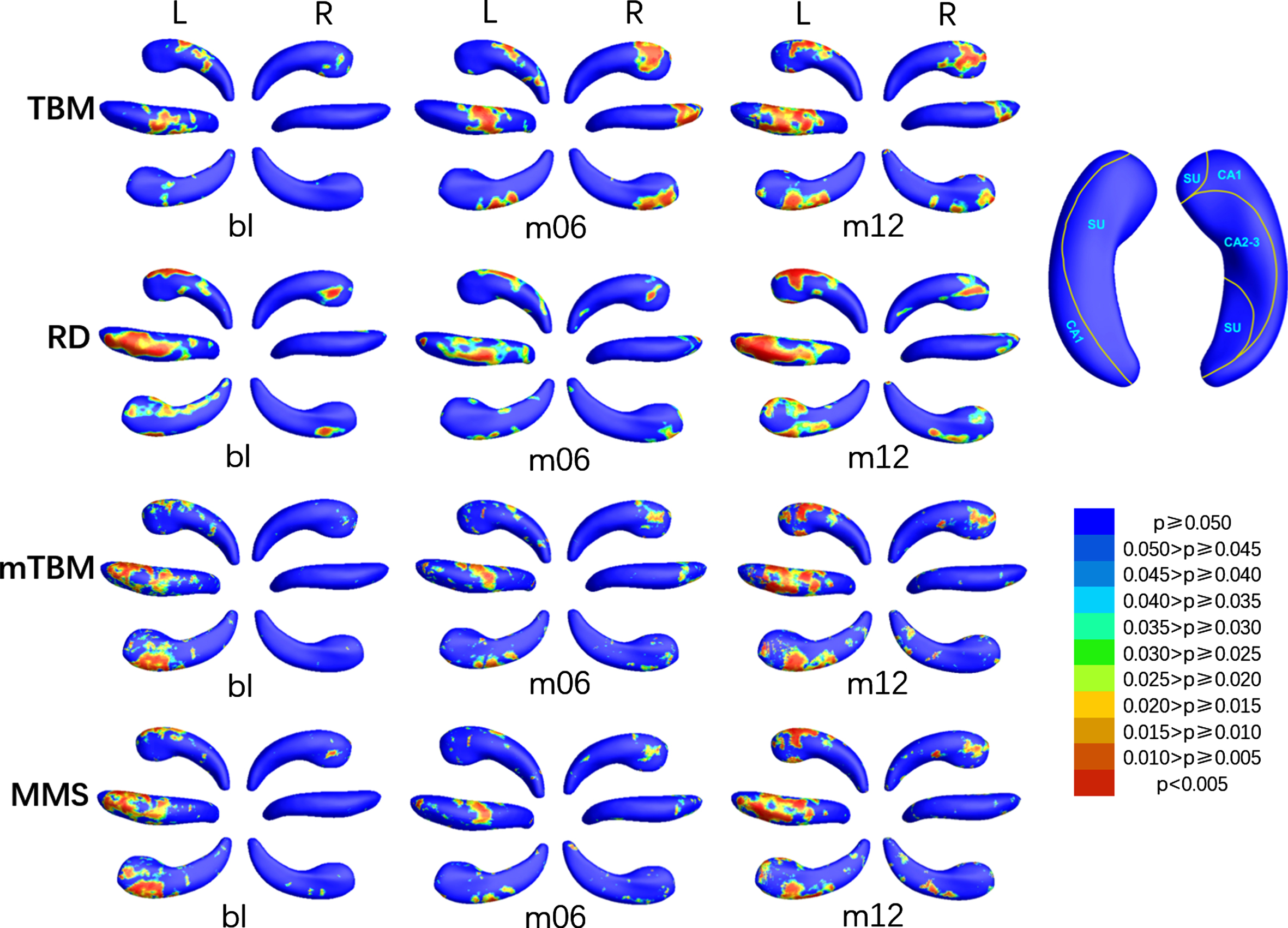
P-map of bilateral hippocampus when comparing MCIs with HC at bl, m06, and m12 using TBM, RD, mTBM, and MMS respectively. SU, subiculum.

Fig. 3

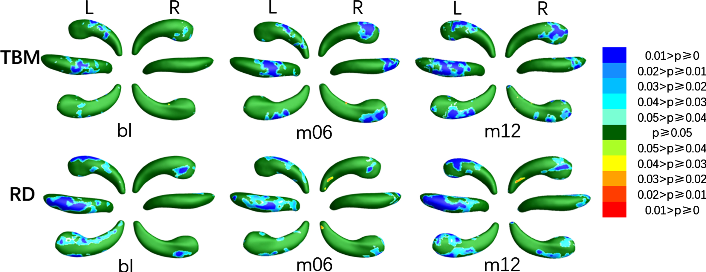
Areas with relative atrophy and expansion of the left and right hippocampus when comparing MCIs with HC at bl, m06, and m12 using TBM and RD respectively.

Table 2

The global p-values of the pairs of the three groups including MCIs and HC, MCIc and MCIs, and MCIc and HC

		MCIs versus HC		MCIc versus HC		MCIc versus MCIs
	L	R	L	R	L	R
bl	TBM	0.2031	0.7247	<0.0001	0.0007	0.0012	<0.0001
	RD	0.0264	0.3652	<0.0001	<0.0001	0.001	0.0001
	mTBM	0.0407	0.799	<0.0001	0.0105	0.0076	0.0149
	MMS	0.037	0.7194	<0.0001	0.0027	0.0037	0.0088
m06	TBM	0.1075	0.0478	<0.0001	0.0002	<0.0001	0.0003
	RD	0.0522	0.1982	<0.0001	0.0005	<0.0001	<0.0001
	mTBM	0.0651	0.1847	<0.0001	0.0175	0.0026	0.0029
	MMS	0.0971	0.2168	<0.0001	0.0031	0.0003	0.0016
m12	TBM	0.0452	0.0391	<0.0001	0.0002	0.0002	0.0002
	RD	0.0165	0.0432	<0.0001	<0.0001	<0.0001	<0.0001
	mTBM	0.034	0.0858	<0.0001	0.0016	<0.0001	0.0007
	MMS	0.0272	0.0592	<0.0001	<0.0001	<0.0001	0.0002

L, left hippocampus; R, right hippocampus; TBM, tensor-based morphometry; RD, radial distance; mTBM, multivariate tensor-based surface morphometry; MMS, the surface multivariate morphometry statistics; p-value in bold, the global significance less than 0.05.

The colored p-map obtained by comparing MCIs with HC were shown in Fig. 4, the relative atrophy or expansion areas were shown in Fig. 5, and the global p-values of the bilateral hippocampus were listed in the fifth and sixth columns of Table 2. The asymmetry of changes in the left and right hippocampus due to disease was more prominent in MCIc. As shown in Fig. 4, the SDAs of TBM in the left hippocampus at bl were distributed in subiculum of the tail part, the dorsal CA1 of the body part and the posterior CA2-3 of the head part, then increased slightly at m06 and m12. The SDAs of RD were mainly distributed in CA1 on the dorsal side, subiculum on the ventral side and CA2-3 near the head part, and gradually extended to the anterior ven subiculum of the anterior middle part. The SDAs of mTBM and MMS were almost distributed throughout the hippocampus from bl, except a few areas of subiculum on the ventral side of the head. Different from the left hippocampus, the SDAs of TBM of the right hippocampus were distributed in dorsal and anterior CA1, posterior subiculum of the tail part, and the ventral subiculum and posterior CA2-3 of the head part. As for RD and MMS, SDAs were distributed in the dorsal and ventral sides of the tail at bl, and expanded with the disease, so that only anterior subiculum of the tail part was not included at m12. The only difference between the SDAs of mTBM and RD was the absence of the CA1 of the tail part on the dorsal side. As illustrated in Fig. 5, almost all SDAs of the bilateral hippocampus was illustrated atrophy while a tiny expansion showed in anterior subiculum on the tail part of the right hippocampus.

Fig. 4

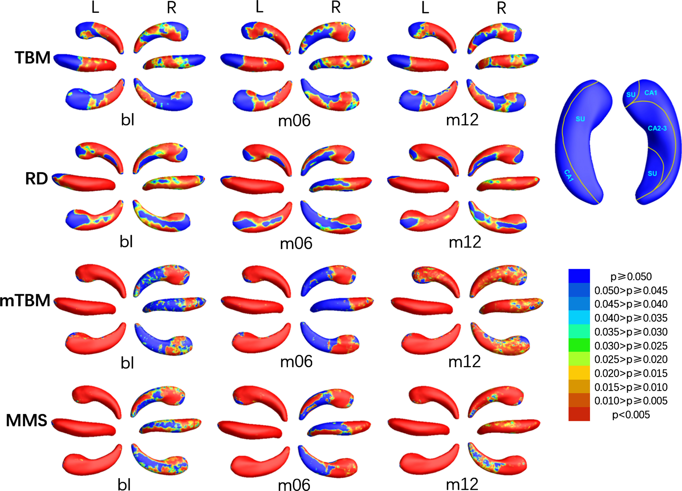
P-map of bilateral hippocampus when comparing MCIc with HC at bl, m06, and m12 using TBM, RD, mTBM, and MMS respectively.

Fig. 5

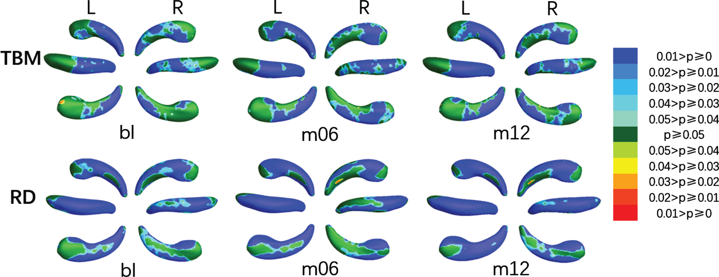
Areas with atrophy and expansion of the left and right hippocampus when comparing MCIc with HC at bl, m06, and m12 using TBM and RD respectively.

We also compared MCIc with MCIs, and the SDAs of which were shown in Fig. 6, the relative atrophy or expansion areas were shown in Fig. 7, and the global p-values of the left and right hippocampus were sorted in the seventh and eighth columns of Table 2. At bl, SDAs of TBM in the left hippocampus were mainly concentrated at the tail part, while the SDAs of RD also emerged in CA1 of the body, and the SDAs of mTBM and MMS scattered on the head part in the meantime. With the course of disease, the SDAs of mTBM and MMS gradually extended, and almost spread all over the left hippocampus at m12, while the SDAs of RD and TBM spread to subiculum and CA2-3 in the head section at m06, and then decreased to the same as which at bl. As for the right hippocampus, SDAs of TBM and RD were mainly distributed in CA1 and subiculum on the dorsal side of the tail and body part and subiculum on the ventral head part, and barely changed with time. The SDAs of mTBM and MMS gradually spread from the dorsal CA1 and CA2-3 and the anterior subiculum of body part to the whole right hippocampus except a tiny area of ventral subiculum of the head part. As shown in Fig. 7, of all the SDAs, expansion exits only in a inappreciable area in subiculum on anterior head part of the left hippocampus, and subiculum of anterior head and CA1 of posterior head of right hippocampus, while atrophy occurred almost throughout the hippocampus.

Fig. 6

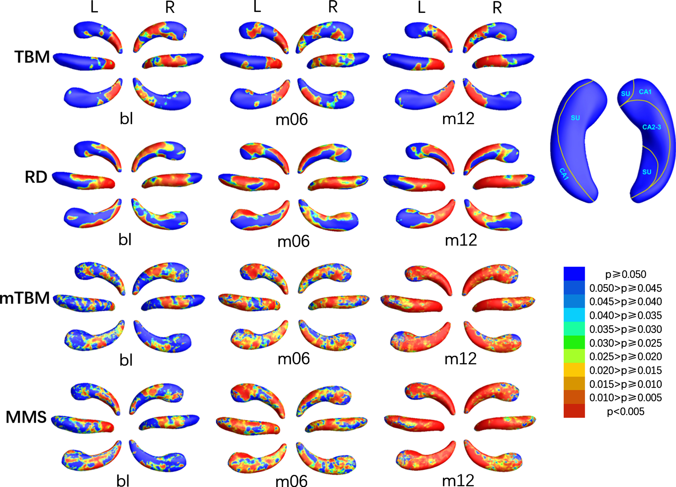
P-map of bilateral hippocampus when comparing MCIc with MCIs at bl, m06, and m12 using TBM, RD, mTBM, and MMS respectively.

Fig. 7

Areas with relative atrophy and expansion of the left and right hippocampus when comparing MCIc with MCIs at bl, m06, and m12 using TBM and RD respectively.

Classification performance

The average of the ten-fold classification results including ACC, SEN, SPE, PPV, and NPV of the most suitable patch size are listed in Table 3. Static features extracted from MRIs at bl, m06, and m12 were used for classification respectively, and the best classification results were achieved at patch size of 35×35. The three feature sets were also combined in pairs to calculate the three dynamic features, and the best classification results of which were obtained at patch size of 35×35. Considering that the information between each feature set may be complementary, we also tested the classification performance on the three feature sets of CD, CS, and CA respectively. The best performance of CD/CS was achieved at patch size of 35×35/30×30, while the most suitable patch size for CA is 25×25.

Table 3

The classification performance of static features, dynamic features, and combined features

		ACC	SEN	SPE	PPV	NPV
Static features	bl	0.8557±0.07	0.7831±0.16	0.9248±0.07	0.8949±0.10	0.8288±0.15
	m06	0.8376±0.12	0.8227±0.19	0.8357±0.15	0.7961±0.18	0.8638±0.14
	m12	0.87±0.06	0.8252±0.07	0.9015±0.10	0.8642±0.10	0.8587±0.10
Dynamic features	D1	0.821±0.09	0.777±0.16	0.8492±0.11	0.8279±0.10	0.8146±0.15
	D2	0.7881±0.08	0.6842±0.21	0.8303±0.15	0.7899±0.15	0.7871±0.10
	D3	0.8143±0.06	0.6627±0.19	0.9289±0.11	0.9044±0.15	0.7843±0.11
Combined features	CS	0.9043±0.09	0.8502±0.13	0.96±0.08	0.9267±0.16	0.8763±0.11
	CD	0.8352±0.06	0.6994±0.16	0.9322±0.08	0.9115±0.10	0.7925±0.12
	CA	0.9176 ± 0.05	0.8535 ± 0.13	0.9789 ± 0.04	0.9633 ± 0.08	0.8809 ± 0.10

ACC, accuracy; SEN, sensitivity; SPE, specificity; PPV, positive predictive value; NPV, negative predictive value; CS/CD/CA, features composed of static features/dynamic features/both static and dynamic features; Values in bold, the highest value in the column.

As shown in Fig. 8, the accuracy of static features outperformed that of the dynamic features, and the accuracy of CS was superior to that of CD. With the combination of all the static features and dynamic features, the accuracy increased markedly, which indicated an effective supplementary of the proposed dynamic features.

Fig. 8

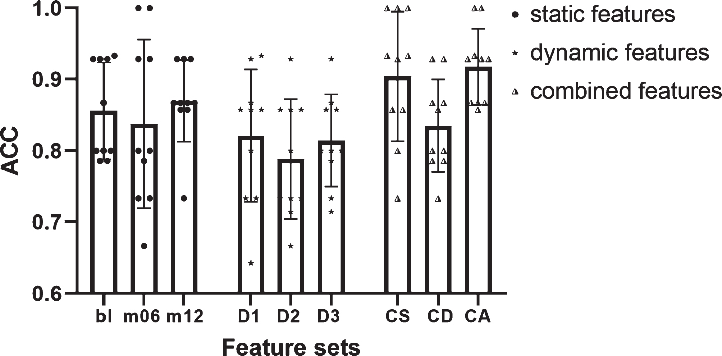
Accuracy of static features, dynamic features, and combined features. Bar heights represented the mean values, with the error bars showing the standard deviations and each symbol indicating one separate accuracy value. Bl/m06/m12, features extracted from MRI at baseline/month 6/month 12; CS/CD/CA, features composed of static features/dynamic features/both static and dynamic features.

DISCUSSION

The findings of this study on pathology mainly include the following four aspects. First, we have uncovered the temporal evolution pattern of lesion in MCIs and MCIc: The atrophy of both MCIc and MCIs are mainly distributed in dorsal CA1, then spread to subiculum and other regions gradually, while the atrophy area of MCIc was larger and more significant. Second, we found that compared with MCIs, MCIc has further atrophy on both left and right hippocampus, and gradually spreads from the dorsal tail part to the entire structure. Third, there was marked asymmetry in the left and right hippocampus of both MCIs and MCIc. Finally, the condition of MCI patients showed a consistent aggravating trend over time, including the increase of significant area and level of significance. It is worth noting that MCIs recovered slightly at m06, which suggested the process of the hippocampal lesion is complicated rather than a simple linear atrophy. As for the classification results, there are two main conclusions. First, the morphological changes in hippocampus contained sensitive and informative features for predicting the conversion of MCI, which showed the central role of hippocampus in the conversion process and the effectiveness of MMS features. Second, the markedly improved accuracy with CA indicated an effective supplementary of the proposed dynamic features and the importance of the temporal evolution information for progressive disease.

In line with previous findings, we found CA1 was the earliest and most significantly atrophied area [59 –61] which progressively spread to the head part [59, 60]. As a highly fragile region, CA1 has been commonly regarded as the main region associated with cognitive process including working memory, spatial memory information processing, and decision making [62 –65]. The atrophied CA1 is thought to reflect the loss of neurons and the neurofibrillary tangles [66 –68], which may directly result in dysmnesia. Montero-Crespo et al. recently reported that the neuronal density in CA1 reduced significantly in AD cases [61]. The lesion area also involved some portion of subiculum then spread to CA2-3 [69, 70], which may be related to the dysfunction of memory retrieval and verbal memory [71, 72].

MCIc was widely considered to be closer to AD while MCIs is closer to HC. Ch $\overset{´}{e}$ telat et al. reported higher rate and accelerated speed of atrophy in CA1 of MCIc compared with MCIs [73], Bozzali et al. found less volume and higher degree atrophy in hippocampus of MCIc than MCIs using VBS method [70], and the ROI-based approach also led to the similar result [74], which was supported by our finding of the further atrophy of MCIc in both left and right hippocampus especially in CA1 compared with MCIs. Combined with the aberrant morphological changes of MCIs and MCIc, we speculated that the specific temporal evolution pattern of hippocampus, including atrophy degree and atrophy region, could provide additional information to predict the conversion from MCI to AD, which was confirmed by the improved prediction performance using the combination of static and dynamic features.

More interestingly, the asymmetry between the left and right hippocampus, which is regarded as a characteristic feature of AD-related deformation, appeared in this study. Specifically, the left hippocampus was demonstrated more affected than the right hippocampus, a phenomenon that has been reported widely in previous studies [38, 74]. Even Csernansky et al. suggested that the CA1 region of the left hippocampus was the only predictor of conversion from MCI to AD [75], which may partly due to that the deformation of the right hippocampus is mainly internal [63].

Another intriguing pattern observed in this study is the recovery at m06 in MCIs, which indicated the resilience of hippocampus and shed a glimmer of hope that MCI patients could return to normal life. Actually, there is a reversion rate of 12.3% per year from MCI to normal [76], which was more optimistic reported in some studies [77, 78]. Kinsella et al. observed the significant improvement of memory performance in participants received memory training [79] and Clare et al reported the resilience in people with cognitive decline [80], which struck a blow to the therapeutic nihilism.

As shown in Fig. 8, as expected, CA had the highest ACC among all feature sets, which supported our hypothesis that the dynamic features supplemented the addition information missing from static features. And the variance of CA (0.05) in the ten-fold cross validation was the smallest of all feature sets. In fact, the stability is just one of the most valued performances in practical application scenarios. As seen in Table 3, the highest values of all performance indicators were found in the CA line, especially with a SPE of 97.89%. While ACC is certainly an important indicator, ACC itself is not necessarily the most concerned indicator in every clinical situation [81]. The excellent SPE and PPV presented by dynamic features fully reflected the abundant information in the temporal evolution pattern, which is of great value to avoid the misdiagnosis of MCIc as much as possible.

An extensive comparison of this method with the recent representative methods, as presented in Table 4, demonstrated our strengths. First, our proposed method achieved excellent performance on a modest sample size. Second, features used in our method were worthy of promotion as its outstanding performance with the only use of morphological information of hippocampus. Finally, there was no need to average the features of the region of interest in the dimensionality reduction pipeline outlined here, which preserved the deformation information of the physiological structure to the maximum extent.

Table 4

Comparison with recent representative methods

Ref	Sample size (MCIs/MCIc)	Features	Dimensionality reduction/selection	Classifier	Performance(%)			Notes
					ACC	SEN	SPE
Moradi [82]	100/164	GM density, age, CM	Regularized logistic regression	Random forest, TSVM	82.0	87.0	74.0	Additional 100 subjects with uMCI were used as inputs for semi-supervised learning, 200 AD and 231 HC for feature selection. The random forest was used for the feature integration, while the TSVM was used for the final classification.
Wei [12]	83/61	CT, CV, CSA, NL, ND	Sparse linear regression	SVM	76.4	65.6	84.3	The authors also compared the classification performance at each point in time, and what we show is the best one in them.
Liu [83]	117/117	GM density	The addition of custom regularization term in the cost function	LSVM, majority voting strategy	79.3	87.9	75.5	The LSVM was used for the classification of every single template based feature set, and the majority voting strategy was used for the final decision.
Minhas [14]	13/16	CM, the volume of entorhinal, fusiform, hippocampus, middle temporal lobe, and the ventricles	The nearest trajectories to the mean feature values	NPC, majority voting strategy	89.7	87.5	92.3	The longitudinal time point readings are used for training the classifier, while only the bl readings were used for validation.
Tong [84]	129/171	grading biomarker sparse represented by the intensities of MRI of HC and AD	Elastic Net method	Random forest	84.1	88.7	76.5	Additional 191 AD and 229 HC subjects were used for feature extraction.
Minhas [85]	65/54	CV, CSA, CT	Wrapper based approach	SVM	84.3	70.4	92.3	The input of the classifier were trajectories of MRI measures calculated by custom regression model.
Gao [86]	129/168	T1 weighed MRI, age	Pre-trained network	Neural network with transfer learning model	76.0	77.0	76.0	Another 1139 HC were used to train the pre-trained model for age prediction, which was transferred by fine-tuned network for conversion prediction.
Shen [87]	59/55	GM volume from MRI, mean intensities from PET images, age	Sparse regression with custom l_2,1-norm	LSVM	78.7	77.3	80.0	Additional 93 AD and 99 HC were used as auxiliary data, which was jointly used with predictor data for feature selection.
Proposed	91/64	RD and mTBM of hippocampus	Patch selection, sparse coding and dictionary learning, and max pooling	Ensemble classifier with tree as the weak learner	91.8	85.4	97.9	None.

GM, grey matter; CM, cognitive measurements; TSVM, transductive support vector machine; uMCI, unknown MCI, whose diagnosis was MCI at baseline but not stable or missing at other time points within 36 months; CT, cortical thickness; CV, cortical volume; CSA, cortical surface area; NL, nodal path length; ND, nodal degree; SVM, support vector machine; LSVM, linear support vector machine; NPC, no parametric classification.

Despite the promising result of this study, there remain several limitations to be addressed for further research. Firstly, in order to include more subjects, the diagnosis in the ADNI database was used as the criteria for inclusion and grouping, while the MMSE scores of a few subjects were missing. Secondly, since the MRI scan and diagnosis every 6 months in a continuous time were required to be all available, the specified stable phase and conversion period were both relatively short, so that some patients assigned to MCIs group may convert to AD after m24, which also has an effect on result. Finally, the age-related change of hippocampus was not taken into account in the comparison between MCI and HC, which may introduce some effect to the results.

Footnotes

ACKNOWLEDGMENTS

This work was supported in part by the National Key Research and Development Program of China (Grant No. 2019YFA0706200), in part by the National Natural Science Foundation of China (Grant No. 61632014, No. 61627808), in part by the Natural Science Foundation of Gansu Province of China (Grant No. 20JR5RA292), and in part by the Department of Education of Gansu Province: “Innovation Star” Project for Excellent Postgraduates (2021CXZX-121).

Data collection and sharing for this project was funded by the Alzheimer’s Disease Neuroimaging Initiative (ADNI) (National Institutes of Health Grant U01 AG024904) and DOD ADNI (Department of Defense award number W81XWH-12-2-0012). ADNI is funded by the National Institute on Aging, the National Institute of Biomedical Imaging and Bioengineering, and through generous contributions from the following: AbbVie, Alzheimer’s Association; Alzheimer’s Drug Discovery Foundation; Araclon Biotech; BioClinica, Inc.; Biogen; Bristol-Myers Squibb Company; CereSpir, Inc.; Cogstate; Eisai Inc.; Elan Pharmaceuticals, Inc.; Eli Lilly and Company; EuroImmun; F. Hoffmann-La Roche Ltd. and its affiliated company Genentech, Inc.; Fujirebio; GE Healthcare; IXICO Ltd.; Janssen Alzheimer Immunotherapy Research & Development, LLC.; Johnson & Johnson Pharmaceutical Research & Development LLC.; Lumosity; Lundbeck; Merck & Co., Inc.; Meso Scale Diagnostics, LLC.; NeuroRx Research; Neurotrack Technologies; Novartis Pharmaceuticals Corporation; Pfizer Inc.; Piramal Imaging; Servier; Takeda Pharmaceutical Company; and Transition Therapeutics. The Canadian Institutes of Health Research is providing funds to support ADNI clinical sites in Canada. Private sector contributions are facilitated by the Foundation for the National Institutes of Health (). The grantee organization is the Northern California Institute for Research and Education, and the study is coordinated by the Alzheimer’s Therapeutic Research Institute at the University of Southern California. ADNI data are disseminated by the Laboratory for Neuro Imaging at the University of Southern California.

Authors’ disclosures available online ().

References

Fan

, Brooks

, Okello

, Edison

(2016) An early and late peak in microglial activation in Alzheimer’s disease trajectory: A longitudinal PET study. Alzheimers Dement 12, 527–528.

Aggleton

, Pralus

, Nelson

AJD

, Hornberger

(2016) Thalamic pathology and memory loss in early Alzheimer’s disease: Moving the focus from the medial temporal lobe to Papez circuit. Brain 139, 1877–1890.

Anderson

(2019) State of the science on mild cognitive impairment (MCI). CNS Spectr 24, 1–10.

Alhurani

, Vassilaki

, Aakre

, Mielke

, Kremers

, Machulda

, Geda

, Knopman

, Peterson

, Roberts

(2016) Decline in weight and incident mild cognitive impairment: Mayo Clinic Study of Aging. JAMA Neurol 73, 439–446.

Zhou

, Suk

, Shen

, Li

(2016) Sparse multi-response tensor regression for Alzheimer’s disease study with multivariate clinical assessments. IEEE Trans Med Imaging 35, 1927–1936.

Chandra

, Dervenoulas

, Politis

(2019) Magnetic resonance imaging in Alzheimer’s disease and mild cognitive impairment. J Neurol 266, 1293–1302.

Guo

, Li

, Zheng

, Huang

, Zhou

, Hu

, Yao

, Hu

(2020) A novel conversion prediction method of MCI to AD based on longitudinal dynamic morphological features using ADNI structural MRIs. J Neurol 267, 2983–2997.

Eskildsen

, Coupé

, García-Lorenzo

, Fonov

, Pruessner

, Collins

(2013) Prediction of Alzheimer’s disease in subjects with mild cognitive impairment from the ADNI cohort using patterns of cortical thinning. Neuroimage 65, 511–521.

Ota

, Oishi

, Ito

, Fukuyama

(2014) A comparison of three brain atlases for MCI prediction. J Neurosci Methods 221, 139–150.

10.

Ferreira

, Diniz

, Forlenza

, Busatto

, Zanetti

(2011) Neurostructural predictors of Alzheimer’s disease: A meta-analysis of VBM studies. Neurobiol Aging 32, 1733–1741.

11.

Tabatabaei-Jafari

, Shaw

, Walsh

, Cherbuin

(2019) Regional brain atrophy predicts time to conversion to Alzheimer’s disease, dependent on baseline volume. Neurobiol Aging 83, 86–94.

12.

Wei

, Li

, Fogelson

, Li

(2016) Prediction of conversion from mild cognitive impairment to Alzheimer’s disease using MRI and structural network features. Front Aging Neurosci 8, 76.

13.

Chupin

, Gérardin

, Cuingnet

, Boutet

, Lemieux

, Lehéricy

, Benali

, Garnero

, Colliot

(2010) Fully automatic hippocampus segmentation and classification in Alzheimer’s disease and mild cognitive impairment applied on data from ADNI. Hippocampus 19, 579–587.

14.

Minhas

, Khanum

, Riaz

, Alvi

, Khan

(2016) A nonparametric approach for mild cognitive impairment to AD conversion prediction: Results on longitudinal data. IEEE J biomed Health Inform 21, 1403–1410.

15.

Hojjati

, Ebrahimzadeh

, Khazaee

, Babajani-Feremi

(2018) Predicting conversion from MCI to AD by integrating rs-fMRI and structural MRI. Comput Biol Med 102, 30–39.

16.

Sun

, Giessen

MVD

, Lelieveldt

BPF

, Staring

(2013) Detection of conversion from mild cognitive impairment to Alzheimer’s disease using longitudinal brain MRI. Front Neuroinformatics 11, 16.

17.

Zhang

, Liu

, An

, Gao

, Shen

(2017) Alzheimer’s disease diagnosis using landmark-based features from longitudinal structural MR images. IEEE J Biomed Health Inform 21, 1607–1616.

18.

Michael

(2013) The hippocampus as a cognitive Map. J Nerv Ment Dis 168, 191–192.

19.

Steele

, Morris

RGM

(2015) Delay-dependent impairment of a matching-to-place task with chronic and intrahippocampal infusion of the NMDA-antagonist D-AP5. Hippocampus 9, 118–136.

20.

Winocur

, Wojtowicz

, Sekeres

, Snyder

, Wang

(2010) Inhibition of neurogenesis interferes with hippocampus-dependent memory function. Hippocampus 16, 296–304.

21.

Wood

, Dudchenko

, Eichenbaum

(1999) The global record of memory in hippocampal neuronal activity. Nature 397, 613–616.

22.

Tian

, Guo

, Sui

, Driskill

, Phensy

, Wang

, Gauba

, Zigman

, Swerdlow

, Kroener

, Du

(2019) Disrupted hippocampal growth hormone secretagogue receptor 1α interaction with dopamine receptor D1 plays a role in Alzheimer^′s disease. Sci Transl Med 11, eaav6278.

23.

Tabatabaei-Jafarimd

, Shaw

, Walsh

, Cherbuin

, Anderson

(2020) Cognitive/functional measures predict Alzheimer’s disease, dependent on hippocampal volume. J Gerontol B Psychol Sci Soc Sci 75, 1393–1402.

24.

Leeuw

, Barkhof

, Scheltens

(2004) White matter lesions and hippocampal atrophy in Alzheimer’s disease. Neurology 62, 310–312.

25.

Gómez-Sancho

, Tohka

, Gómez-Verdejo

(2018) Comparison of feature representations in MRI-based MCI-to-AD conversion prediction. Magn Reson Imaging 50, 84–95.

26.

Ballmaier

, Narr

, Toga

, Elderkin-Thompson

, Thompson

, Hamilton

, Haroon

, Pham

, Heinz

, Kumar

(2008) Hippocampal morphology and distinguishing late-onset from early-onset elderly depression. Am J Psychiat 165, 229–237.

27.

Dudek

, Alexander

, Farris

(2016) Rediscovering area CA2: Unique properties and functions. Nat Rev Neurosci 17, 89–102.

28.

Han

, Xu

, Prince

(2003) A topology preserving level set method for geometric deformable models. IEEE Trans Pattern Anal Mach Intell 25, 755–768.

29.

Lorensen

, Cline

(1987) Marching cubes: A high resolution 3D surface construction algorithm. Comput Graph 21, 163–169.

30.

Shi

, Thompson

, Gutman

, Wang

(2013) Surface fluid registration of conformal representation: Application to detect disease burden and genetic influence on hippocampus. Neuroimage 78, 111–134.

31.

, Zhang

, Li

, Shi

, Zou

, Guo

, Li

, Yao

, Wang

, Hu

(2020) A novel pipeline leveraging surface-based features of small subcortical structures to classify individuals with autism spectrum disorder. Prog Neuropsychopharmacol Biol Psychiatry 104, 109989.

32.

Hoppe

(1996) Progressive meshes. Proceedings of the 23rd Annual Conference on Computer Graphics and Interactive Techniques, Association for Computing Machinery, pp. 99–108.

33.

Loop

(1987) Smooth subdivision surfaces based on triangles. Masters thesis, University of Utah, Department of Mathematics.

34.

Wang

, Gu

, Chan

, Thompson

, Yau

(2008) Conformal slit mapping and its applications to brain surface parameterization. Med Image Comput Comput Assist Interv 11(Pt 1), 585–593.

35.

Wang

, Lui

, Gu

, Hayashi

, Chan

, Toga

, Thompson

, Yau

(2007) Brain surface conformal parameterization using Riemann surface structure. IEEE Trans Med Imaging 26, 657–665.

36.

Leow

, Huang

, Geng

, Becker

, Davis

, Toga

, Thompson

(2005) Inverse consistent mapping in 3D deformable image registration: Its construction and statistical properties. Biennial International Conference on Information Processing in Medical Imaging, pp. 493–503.

37.

Wang

, Panigrahy

, Shi

, Ceschin

, Marvin

, Nelson , Gutman

, Thompson

, Leporé

(2013) Surface multivariate tensor-based morphometry on premature neonates: A pilot study. Miccai Workshop on Image Analysis of Human Brain Development.

38.

Thompson

, Hayashi

, Zubicaray

, Janke

, Rose

, Semple

, Hong

, Herman

, Gravano

, Doddrell

, Toga

(2004) Mapping hippocampal and ventricular change in Alzheimer disease. Neuroimage 22, 1754–1766.

39.

Chung

, Dalton

, Davidson

(2008) Tensor-based cortical surface morphometry via weighted spherical harmonic representation. IEEE Trans Med Imaging 27, 1143–1151.

40.

Wang

, Chan

, Toga

, Thompson

(2009) Multivariate tensor-based brain anatomical surface morphometry via holomorphic one-forms . International Conference on Medical Image Computing & Computer-assisted Intervention: Part I, pp. 337–344.

41.

Stonnington

, Wu

, Zhang

, Shi

, Bauer-III

, Devadas

, Su

, Locke

DEC

, Reiman

, Caselli

, Chen

, Wang

(2021) Improved prediction of imminent progression to clinically significant memory decline using surface multivariate morphometry statistics and sparse coding. J Alzheimers Dis 81, 209–220.

42.

Yao

, Fu

, Wu

, Zhang

, Yu

, Zhang

, Wu

, Wang

, Hu

(2018) Morphological changes in subregions of hippocampus and amygdala in major depressive disorder patients. Brain Imaging Behav 14, 653–667.

43.

Zhang

, Stonnington

, Li

, Shi

, Bauer

, Gutman

, Chen

, Reiman

, Thompson

, Ye

, Wang

(2016) Applying sparse coding to surface multivariate tensor-based morphometry to predict future cognitive decline. 2016 IEEE 13th International Symposium on Biomedical Imaging (ISBI), pp. 646–650.

44.

Hotelling

(1992) The generalization of student’s ratio. In Breakthroughs in Statistics. Springer Series in Statistics (Perspectives in Statistics), Kotz

, Johnson

, eds. Springer, New York, NY.

45.

Styner

, Oguz

, Xu

, Brechbühler

, Pantazis

, Levitt

, Shenton

, Gerig

(2006) Statistical shape analysis of brain structures using SPHARM-PDM. Insight J Miccai 2006 Opensource Workshop.

46.

, Dong

, Gui

, Zhang

, Su

, Chen

, Thompson

, Caselli

, Reiman

, Ye

, Wang

(2020) Predicting brain amyloid using multivariate morphometry statistics, sparse coding, and correntropy: Validation in 1,125 individuals from the ADNI and OASIS databases. J Alzheimers Dis 81, 209–220.

47.

Dong

, Zhang

, Stonnington

, Wu

, Gutman

, Chen

, Su

, Baxter

, Thompson

, Reiman

, Caselli

, Wang

(2020) Applying surface-based morphometry to study ventricular abnormalities of cognitively unimpaired subjects prior to clinically significant memory decline. Neuroimage Clin 27, 102338.

48.

Wade

BSC

, Joshi

, Gutman

, Thompson

(2016) Machine learning on high dimensional shape data from subcortical brain surfaces: A comparison of feature selection and classification methods. Pattern Recognit 9352, 36–43.

49.

, Zhang

, Shi

, Chen

, Caselli

, Reiman

, Wang

(2018) Hippocampus morphometry study on pathology-confirmed Alzheimer’s disease patients with surface multivariate morphometry statistics. 2018 IEEE 15th International Symposium on Biomedical Imaging (ISBI 2018), pp. 1555–1559.

50.

Lin

, Li

, Sun

, Lai

, Davidson

, Fan

, Ye

(2014) Stochastic coordinate coding and its application for Drosophila gene expression pattern annotation. arXiv preprint arXiv:1407.8147.

51.

Mairal

, Bach

, Ponce

, Sapiro

(2009) Online dictionary learning for sparse coding. Proceedings of the 26th Annual International Conference on Machine Learning, pp. 689–696.

52.

Olshausen

, Field

(1997) Sparse coding with an overcomplete basis set: A strategy employed by V1? Vision Res 37, 607–609.

53.

Lee

, Little

, Raina

, Ng

(2007) Efficient sparse coding algorithms. Advances in Neural Information Processing Systems, pp. 801–808.

54.

Boureau

Y-L

, Ponce

, LeCun

(2010) A theoretical analysis of feature pooling in visual recognition. Proceedings of the 27th international conference on machine learning (ICML-10), pp. 111–118.

55.

Rodriguez

, Kuncheva

, Alonson C

(2006) Rotation forest: A new classifier ensemble method. IEEE Trans Pattern Anal Mach Intell 28, 1619–1630.

56.

Pratama

, Pedrycz

, Lughofer

(2017) Evolving ensemble fuzzy classifier. IEEE Trans Fuzzy Syst 26, 2552–2567.

57.

Freund

, Schapire R

(1997) A decision-theoretic generalization of on-line learning and an application to boosting. J Comput Syst Sci 55, 119–139.

58.

Friedman

(2001) Greedy function approximation: A gradient boosting machine. Ann Stat 29, 1189–1232.

59.

Csernansky

, Wang

, Joshi

, Miller

, Gado

, Kido

, Mckeel

, Morris

, Miller

(2000) Early DAT is distinguished from aging by high-dimensional mapping of the hippocampus. Dementia of the Alzheimer type. Neurology 55, 1636–1643.

60.

Wang

, Swank

, Glick

, Gado

, Miller

, Morris

, Csernansky

(2003) Changes in hippocampal volume and shape across time distinguish dementia of the Alzheimer type from healthy aging. Neuroimage 20, 667–682.

61.

Montero-Crespo

, Domínguez-Álvaro

, Alonso-Nanclares

, Defelipe

, Blazquez-Llorca

(2020) Three-dimensional analysis of synaptic organization in the hippocampal CA1 field in Alzheimer’s disease. Brain 44, 553–573.

62.

Benchenane

, Peyrache

, Khamassi

, Tierney

, Gioanni

, Battaglia

, Wiener

(2010) Coherent theta oscillations and reorganization of spike timing in the hippocampal- prefrontal network upon learning. Neuron 66, 921–936.

63.

Chandrasekaran

, Choi

, Arvas

, Salimian

, Singh

, Xu

, Gullapalli

, Kristian

, Russell

(2020) Nicotinamide mononucleotide administration prevents experimental diabetes-induced cognitive impairment and loss of hippocampal neurons. Int J Mol Sci 21, 3756.

64.

Cohen

, Munchow

, Rios

, Zhang

, Asgeirsdóttir

, Stackman

(2013) The rodent hippocampus is essential for nonspatial object memory. Curr Biol 23, 1685–1690.

65.

Platano

, Fattoretti

, Balietti

, Giorgetti

, Casoli

, Stefano

, Bertoni-Freddari

, Aicardi

(2008) Synaptic remodeling in hippocampal CA1 region of aged rats correlates with better memory performance in passive avoidance test. Rejuv Res 11, 341–348.

66.

Gunten

, Kvari

, Bussière

, Rivara

C-B

, Gold

, Bouras

, Hof

, Giannakopoulos

(2006) Cognitive impact of neuronal pathology in the entorhinal cortex and CA1 field in Alzheimer’s disease. Neurobiol Aging 27, 270–277.

67.

Zarow

, Vinters

, Ellis

, Weiner

, Mungas

, White

, Chui

(2010) Correlates of hippocampal neuron number in Alzheimer’s disease and ischemic vascular dementia. Ann Neurol 57, 896–903.

68.

Kril

, Patel

, Harding

, Halliday

(2002) Neuron loss from the hippocampus of Alzheimer’s disease exceeds extracellular neurofibrillary tangle formation. Acta Neophilol 103, 370–376.

69.

Apostolova

, Dinov

, Dutton

, Hayashi

, Toga

, Cummings

, Thompson

(2006) 3D comparison of hippocampal atrophy in amnestic mild cognitive impairment and Alzheimer’s disease. Brain 129, 2867–2873.

70.

Bozzali

, Filippi

, Magnani

, Cercignani

, Franceschi

, Schiatti

, Castiglioni

, Mossini

, Falautano

, Scotti

(2006) The contribution of voxel-based morphometry in staging patients with mild cognitive impairment. Neurology 67, 453–460.

71.

Eldridge

, Engel

, Zeineh

, Bookheimer

, Hnowlton

(2005) A dissociation of encoding and retrieval processes in the human hippocampus. J Neurosci 25, 3280–3286.

72.

Mori

, Yoneda

, Yamashita

, Hirono

, Ikeda

, Yamadori

(1997) Medial temporal structures relate to memory impairment in Alzheimer’s disease: An MRI volumetric study. J Neurol 63, 214–221.

73.

Chételat

, Fouquet

, Kalpouzos

, Denghien

, Sayette

VDI

, Viader

, Mézenge

, Landeau

, Baron

, Eustache

, Desgranges

(2008) Three-dimensional surface mapping of hippocampal atrophy progression from MCI to AD and over normal aging as assessed using voxel-based morphometry. Neuropsychologia 46, 1721–1731.

74.

Chetelat

, Baron

J-C

(2003) Early diagnosis of Alzheimer’s disease: Contribution of structural neuroimaging. Neuroimage 18, 525–541.

75.

Csernansky

, Wang

, Swank

, Miller

, Gado

, Mckeel

, Miller

, Morris

(2005) Preclinical detection of Alzheimer’s disease: Hippocampal shape and volume predict dementia onset in the elderly. Neuroimage 25, 783–792.

76.

Roberts

, Geda

, Knopman

, Cha

, Pankratz

, Boeve

, Tangalos

, Ivnlk

, Rocca

, Petersen

(2012) The incidence of MCI differs by subtype and is higher in men: The Mayo Clinic study of aging. Neurology 78, 342–351.

77.

Manly

, Tang

, Schupf

, Stern

, Vonsattel

JPG

, Mayeux

(2010) Frequency and course of mild cognitive impairment in a multiethnic community. Ann Neurol 63, 494–506.

78.

Boyle

, Buchman

, Barnes

, Bennett

(2010) Effect of a purpose in life on risk of incident Alzheimer disease and mild cognitive impairment in community-dwelling older persons. Arch Gen Psychiatry 67, 304–310.

79.

Kinsella

, Mullaly

, Rand

, Ong

, Burton

, Price

, Phillips

, Storey

(2009) Early cognitive intervention for MCI: A randomized controlled trial. J Neurol Neurosurg Psychiatry 80, 730–736.

80.

Clare

, Kinsella

, Logsdon

, Whitlatch

, Zarit

(2011) Building resilience in mild cognitive impairment and early-stage dementia: Innovative approaches to intervention and outcome evaluation. Resilience in Aging, pp. 245–259.

81.

Cuker

, Gimotty

, Crowther

, Warkentin

(2012) Predictive value of the 4Ts scoring system for heparin-induced thrombocytopenia: A systematic review and meta-analysis. Blood 120, 4160–4167.

82.

Moradi

, Pepe

, Gaser

, Huttunen

, Tohka

(2015) Machine learning framework for early MRI-based Alzheimer’s conversion prediction in MCI subjects. Neuroimage 104, 398–412.

83.

Liu

, Zhang

, Shen

(2016) Relationship induced multi-template learning for diagnosis of Alzheimer’s disease and mild cognitive impairment. IEEE Trans Med Imaging 35, 1463–1474.

84.

Tong

, Gao

, Guerrero

, Ledig

, Chen

, Rueckert

(2016) A novel grading biomarker for the prediction of conversion from mild cognitive impairment to Alzheimer’s disease. IEEE Trans Biomed Eng 64, 155–165.

85.

Minhas

, Khanum

, Riaz

, Khan

, Alvi

(2017) Predicting progression from mild cognitive impairment to Alzheimer’s disease using autoregressive modelling of longitudinal and multimodal biomarkers. IEEE J Biomed Health Inform 22, 818–825.

86.

Fei

, Yoon

, Xu

, Goradia

, Luo

, Wu

, Su

(2020) AD-NET: Age-adjust neural network for improved MCI to AD conversion prediction. Neuroimage Clin 27, 102290.

87.

Shen

, Zhu

, Zhang

, Wang

, Chen

, Xv

, Shao

(2021) Heterogeneous data fusion for predicting mild cognitive impairment conversion. Inf Fusion 66, 54–63.